Identification and Prediction of Internet Traffic Using Artificial Neural ...

J. Intelligent Learning Systems & Applications, 2010, 2, 147-155

147

doi:10.4236/jilsa.2010.23018 Published Online August 2010 (http://www.SciRP.org/journal/jilsa)

Identification and Prediction of Internet Traffic Using Artificial Neural Networks Samira Chabaa1, Abdelouhab Zeroual1, Jilali Antari1,2 1

Department of Physics Cadi Ayyad University, Faculty of Sciences Semlalia, Marrakech, Morocco; 2Ibn Zohr University-Agadir, Polydisciplinaire Faculty of Taroudant, Morocco. Email: [email protected] Received March 16th, 2010; revised July 16th, 2010; accepted July 25th, 2010.

ABSTRACT This paper presents the development of an artificial neural network (ANN) model based on the multi-layer perceptron (MLP) for analyzing internet traffic data over IP networks. We applied the ANN to analyze a time series of measured data for network response evaluation. For this reason, we used the input and output data of an internet traffic over IP networks to identify the ANN model, and we studied the performance of some training algorithms used to estimate the weights of the neuron. The comparison between some training algorithms demonstrates the efficiency and the accuracy of the Levenberg-Marquardt (LM) and the Resilient back propagation (Rp) algorithms in term of statistical criteria. Consequently, the obtained results show that the developed models, using the LM and the Rp algorithms, can successfully be used for analyzing internet traffic over IP networks, and can be applied as an excellent and fundamental tool for the management of the internet traffic at different times. Keywords: Artificial Neural Network, Multi-Layer Perceptron, Training Algorithms, Internet Traffic

1. Introduction Recently, much attention has been paid to the topic of complex networks, which characterize many natural and artificial systems such as internet, airline transport systems, power grid infrastructures, and the World Wide Web [1-3]. Indeed, Traffic modeling is fundamental to the network performance evaluation and the design of network control scheme which is crucial for the success of high-speed networks [4]. This is because network traffic capacity will help each webmaster to optimize their website, maximize online marketing conversions and lead campaign tracking [5,6]. Furthermore, monitoring the efficiency and performance of IP networks based on accurate and advanced traffic measurements is an important topic in which research needs to explore a new scheme for monitoring network traffic and then find out its proper approach [7]. So, a traffic model with a simple expression is significant, which is able to capture the statistical characteristics of the actual traffic accurately. Since the 1950s, many models have been developed to study complex traffic phenomena [5]. The need for accurate traffic parameter prediction has long been recognized in the international scientific literature [8]. The main motivation here is to obtain a better understanding of the characteristics of the network traffic. One Copyright © 2010 SciRes.

of the approaches used for the preventive control is to predict the near future traffic in the network and then take appropriate actions such as controlling buffer sizes [9]. Several works developed in the literature are interested to resolve the problem of improving the efficiency and effectiveness of network traffic monitoring by forecasting data packet flow in advance. Therefore, an accurate traffic prediction model should have the ability to capture the prominent traffic characteristics, e.g. shortand long- range dependence, self-similarity in large-time scale and multifractal in small-time scale [10]. Several traffic prediction schemes have been proposed [11,19]. Among the proposed schemes on traffic prediction, neural network (NN) based schemes brought our attention since NN has been shown more than acceptable performance with relatively simple architecture in various fields [19-17]. Neural networks (NNs) have been successfully used for modeling complex nonlinear systems and forecasting signals for a wide range of engineering applications [20-26]. Indeed, the literature has shown that neural networks are one of the best alternatives for modeling and predicting traffic parameters possibly because they can approximate almost any function regardless of its degree of nonlinearity and without prior knowledge of its functional form [27]. Several researchers have demJILSA

148

Identification and Prediction of Internet Traffic Using Artificial Neural Networks

onstrated that the structure of neural network is characterized by a large degree of uncertainty which is presented when trying to select the optimal network structure. The most distinguished character of a neural network over the conventional techniques in modeling nonlinear systems is learning capability [19]. The neural network can learn the underlying relationship between input and output of the system with the provided data [19-26]. Among the various NN-based models, the feed-forward neural network, also known as the Multi Layer Perceptron Type Neural Network (MLPNN), is the most commonly used and has been applied to solve many difficult and diverse problems [27-30]. The aim of this paper is to use artificial neural networks (ANN) based on the multi-layer perceptron (MLP) for identifying and developing a model that is able to analyze and predict the internet traffic over IP networks by comparing some training algorithms using statistical criteria.

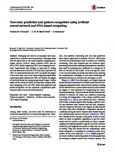
2. Artificial Neural Networks Artificial neural networks (ANN) are an abstract simulation of a real nervous system that consists of a set of neural units connected to each other via axon connections which are very similar to the dendrites and the axons in biological nervous systems [31]. Furthermore, artificial neural networks are a large class of parallel processing architecture which can mimic complex and nonlinear processing units called neurons [32]. An ANN, as function approximator, is useful because it can approximate a desired behavior without the need to specify a particular function. This is a big advantage of artificial neural networks compared to multivariate statistics [33]. ANN can be trained to reach, from a particular input, a specific target output using a suitable learning method until the network output matches the target [34]. In addition, neural networks are trained by experience, when an unknown input is applied to the network it can generalize from past experiences and product a new result [35-37]. ANN is constituted by a tree layer: an input layer, an output layer, and an intermediate hidden layer, with their corresponding neurons. Each layer is connected to the next layer with a neuron giving rise to a large number of connections. This architecture allows ANNs to learn complicated patterns. Each connection has a weight associated with it. The hidden layer learns to provide a representation for the inputs. The output of a neuron in a hidden or output layer is calculated by applying an activation function to the weighted sum of the input to that neuron [20] (Figure 1). ANN model must first be “trained” by using cases with known outcomes and it will then adjust its weighting of various input variables over time to refine the output data [10]. The validation data Copyright © 2010 SciRes.

Figure 1. Neural network model

are used for evaluating the performance of the ANN model. In this work, we used the back-propagation based Multi Layer Perceptron (MLP) neural network. The multi layer perceptron is the most frequently used neural network technique, which makes it possible to carry out the most various applications. The identification of the MLP neural networks requires two types of stages. The first is the determination of the network structure. Different networks with one layer hidden have been tried, and the activation function used in this study is the sigmoid function described as: f ( x) 

1 1  exp ( x)

(1)

The second stage is the identification of parameters (learning of the neural networks). The suite of the used back-propagation neural networks are part of the MATLAB neural network toolbox which assisted in appraising each of the above individual neural network models for predictive purposes [38,39]. In this study various training algorithms are used.

3. Training Algorithms The MLP network training can be viewed as a function approximation problem in which the network parameters (weights and biases) are adjusted during the training, in an effort to minimize (optimize) error function between the network output and the desired output [40]. The issue of learning algorithm is very important for MLP neural network [41]. Most of the well known ANN training algorithms are based on true gradient computations. Among these, the most popular and widely used ANN training algorithm is the Back Propagation (BP) [42,43]. The BP method, also known as the error back propagation algorithm, is based on the error correlation learning rule [44]. The BP neural networks are trained with different training algorithms. In this section we describe some of these algorithms. The BP algorithm uses the gradients of the activation functions of neurons in order to backJILSA

Identification and Prediction of Internet Traffic Using Artificial Neural Networks

propagate the error that is measured at the output of a neural network and calculate the gradients of the output error over each weight in the network. Subsequently, these gradients are used in updating the ANN weights [45].

3.1 Gradient Descent Algorithm The standard training process of the MLP can be realized by minimizing the error function E defined by:



E   p 1  j M1 y Mj, p  t j , p p

N

  2

p p 1

Ep

(2)

where y Mj, p  t j , p is the squared difference between the actual output value at the jth output layer neuron for pattern p and the target output value. The scalar p is an index over input–output pairs. The general purpose of the training is to search an optimal set of connection weights in the manner that the errors of the network output can be minimized [46]. In order to simplify the formulation of the equations, let w be the n-dimensional weight vector of all connection weights and biases. Accordingly, the weight update equation for any training algorithm has the iterative form. In each iteration, the synaptic weights are modified in the opposing direction to those of the gradient of the cost function. The on-line or off-line versions are applied where we use the instantaneous gradient of the partial error function Ep, or on the contrary the gradient of the total error function E respectively. To calculate the gradient for the two cases, the Error Back Propagation (EBP) algorithm is applied. The procedure in the mode off-line sums up as follows w  k  1  w  k    k d k

where, w  k    w1  k  ,... ... .., wn  k  

T

(3) is the weight

vector in k iterations, n is the number of synaptic connections of the network, k is the index of iteration,  k is the learning rate which adjusts the size of the step gradient, and dk is a search direction which satisfies the descent condition. The steepest descent direction is based to minimize the error function, namely d k   g w T

 E E  where g w  k    ,... ... ... ..,  is the grawn  k    w1  k  dient of the estimated error in w. throughout the training with the standard steepest descent, the learning rate is held constant, which makes the algorithm very sensitive to the proper setting of the learning rate. Indeed, the algorithm may oscillate and become unstable, if the learning rate is set too high. But, if the learning rate is too small, the algorithm will take a long time to converge. Copyright © 2010 SciRes.

149

3.2 Conjugate Gradient Algorithm The basic back propagation algorithm adjusts the weights in the steepest descent direction in which the performance function decreases most rapidly. Although, the function decreases most rapidly along the negative of the gradient, this does not necessarily produce the fastest convergence [44]. In the conjugate gradient algorithms, a search is made along the conjugate gradient direction to determine the step size which will minimize the performance function along that line [41]. The conjugate gradient (CG) methods are a class of very important methods for minimizing smooth functions, especially when the dimension is large [47]. The principal advantage of the CG is that they do not require the storage of any matrices as in Newton’s method, or as in quasi-Newton methods, and they are designed to converge faster than the steepest descent method [46]. There are four types of conjugate gradient algorithms which can be used for training. All of the conjugate gradient algorithms start out by searching in the steepest descent direction (negative of the gradient) on the first iteration [41,44,46]: p0 = –gw(0) where p0 is the initial search gradient and g0 is the initial gradient. A line search is then performed to determine the optimal distance to move along the current search direction: w  k  1  w  k    k d k

The next search direction is determined so that it is conjugated to previous search directions. The general procedure for determining the new search direction is to combine the new steepest descent direction with the previous search direction: d k   g w  k    k d k 1

where  k is a parameter to be determined so that d k becomes the k-the conjugate direction. The way in which the  k constant is computed distinguishes the various versions of conjugate gradient, namely Fletcher-Reeves updates (Cgf), Conjugate gradient with Polak-Ribiere updates (Cgp), Conjugate gradient with Powell-Beale restarts (Cgb) and scaled conjugate gradient algorithm (Scg). 1) Conjugate gradient with Fletcher-Reeves updates The procedure to evaluate the constant  k with the Fletcher-Reeves update is [48]

k 

g wT  k  g w  k 

g wT  k  1 g w  k  1

 k represents the ratio of the norm squared of the JILSA

Identification and Prediction of Internet Traffic Using Artificial Neural Networks

150

current gradient to the norm squared of the previous gradient. 2) Conjugate gradient with Polak-Ribiere updates The constant  k is computed by the Polak-Ribiére update as [49]:

k 

g wT  k  yk

g wT  k  1 g w  k  1

where yk  g w  k   g w  k  1 is the inner product of the previous change in the gradient with the current gradient divided by the norm squared of the previous gradient. 3) Conjugate gradient with Powell-Beale restarts In conjugate gradient algorithms, the search direction is periodically reset to the negative of the gradient. The standard reset point occurs when the number of iterations is equal to the number of network parameters (weights and biases), but there are other reset methods that can improve the efficiency of the training process [50]. This technique restarts if there is a very little orthogonality left between the current and the previous gradient: g wT  k  1 g w  k   0.2 g w  k 

2

If this condition is satisfied, the search direction is reset to the negative of the gradient [41,44,51]. 4) Scaled conjugate gradient (Scg) The scaled conjugate gradient algorithm requires a line search at any iteration which is computationally expensive since it requires computing the network response for all training inputs at several times for each search. The Scg combines the model-trust region approach (used in the Levenberg-Marquardt algorithm described in the following section), with the conjugate gradient approach. This algorithm was designed to avoid the time-consuming line search. It is developed by Moller [52], where the constant  k is computed by: g w  k  1  g 2

k 

 k  1 g w  k  2 gw  k  T w

3.3 One Step Secant Battiti proposes a new memory-less quasi-Newton method named one step secant (OSS) [53], which is an attempt to bridge the gap between the conjugate gradient algorithms and the quasi-Newton (secant) algorithms. This algorithm does not store the complete Hessian matrix. It assumes that at any iteration, the previous Hessian was the identity matrix. This has the additional advantage that the new search direction can be calculated without computing a matrix inverse [41,44].

3.4 Levenberg-Marquardt Algorithm The Levenberg-Marquardt (LM) algorithm [54,55] is the Copyright © 2010 SciRes.

most widely used optimization algorithm. It is an iterative technique that locates the minimum of a multivariante function that is expressed as the sum of squares of non linear real valued functions [56-58]. The LM is the first algorithm shown to be blend of steepest gradient descent and Gauss-Newton iterations. Like the quasi-Newton methods, the LM algorithm was designed to approach second-order training speed without having to compute the Hessian matrix [44]. The LM algorithm provides a solution for non linear least squares minimization problems. When the performance function has the form of a sum of squares, then the Hessian matrix can be approximated as [44]: H  JT J

where J is the Jacobian matrix that contains the first derivates of network errors and the gradient can be computed as: gw  JT e

where the Jacobian matrix contains the first derivatives of the network errors with respect to the weights and biases, and e is a vector of network errors. The Levenberg–Marquardt (LM) algorithm uses the approximation to the Hessian matrix in the following Newton-like update [41,44]: 1

wk 1  wk   J T J   I  J T e

where I is the identity matrix and µ is a constant. µ decreases after each successful step (reduction in performance function) and increases only when a tentative step would increase the performance function. In this way, the performance function will always be reduced at each iteration of the algorithm [44].

3.5. Resilient back Propagation (Rp) Algorithm There has been a number of refinements made to the BP algorithm with arguably the most successful in general being the Resilient Back Propagation method or Rp [59-61]. Furthermore, the goal of the algorithm of Rp is to eliminate the harmful effects of the magnitudes of the partial derivatives. Therefore, only the sign of the derivative is used to determine the direction of the weight update. Indeed, the Rp modifies the size of the weight step that is adaptively taken. The adaptation mechanism in Rp does not take into account the magnitude of the gradient ( g w  k  ) as seen by a particular weight, but only the sign of the gradient (positive or negative) [44,61]. The Rp algorithm is based on the modification of each weight by the update value (or learning parameter) in such a way as to decrease the overall error. The update value for each weight and bias is increased whenever the derivative of the performance function with respect to that weight has the same sign for two successive iterations. JILSA

Identification and Prediction of Internet Traffic Using Artificial Neural Networks

151

of the developed model. The accuracy of correlations relative to the measured values is determinated by various statistical means. The criteria exploited in this study were the Root Mean Square Error (RMSE), the Scatter Index (SI), the Relative Error and Mean Absolute Percentage Error (MAPE) [64-66] given by:

The principle of this method is as follows: wk  wk 1   sign  g w  k  1   k  k  n   k 1 if g w  k  1 * g w  k   0  k  n   k 1 if g w  k  1 * g w  k   0



2  R error  E   yˆ m  ym  / ym2 

else  k   k 1 where 0  n   1  n   k is the update value of the weight, which evolves according to changes of sign of the difference ( wk  w k 1 ) of the same weight in k iterations. The update values and the weights are changed after each iteration. All update values are initialized to the value D0. The update value is modified in the following manner: if the current gradient ( g w  k  ) multiplied by the gradient of the previous step is positive (that is the gradient direction has remained the same), then the update value is multiplied by a value n  (which is greater than one). Similarly, if the gradient product is negative, the update value is multiplied by the value n  (which is less than one) [61].

4. Results and Discussion In this part, we are interested in appling the MPL neural networks for developing a model able to identify and predict the internet traffic. The considered data are composed of 1000 points (Figure 2). The databases were divided in two parts training (750 points) and testing (250 points) data as required by the application of MLP. Additionally, the training data set is used to train the MLP and must have enough size to be representative for overall problem. The testing data set should be independent of the training set and are used to assess the classification accuracy of the MLP after the training process [62,63]. The error analysis was used to check the performance

RMSE =

1 N

SI  MAPE 



1/ 2

  

 m 1  ym  yˆ m 

2

N

(2) (3)

RMSE ym

(4)

100 N  i 1 ym  yˆ m N

(5)

where ym and yˆ m represent respectively real and estimated data, ym is the mean values of real data and N represents the sample size. Table 1 shows the obtained results of each statistical indicator for the different algorithms: From these results, we conclude that the Levenberg-Marquardt (LM) and the Resilient back propagation (Rp) algorithms give more precision using the statistical criteria than the other training algorithms. The Gd, Scg, Cgf, Cgp, Cgb and Oss training algorithm give big values in term of the used statistical criteria, which prove that these training algorithms are not significant for prediction purpose. For this reason, we used the LM and the Rp training algorithms in the next paragraph. To agreement the efficiency of the developed model based on the LM and the Rp training algorithms, we draft in Figure 3 the evolution of measured and predicted time series of the internet traffic for the two algorithms where we represent just 100 points. We notice that the two time series have the same behaviour. Table 1. Values of different statistical indicators for different algorithms

0.13 0.12

Training algorithms

Rerror

RMSE

SI

MAPE

0.1

LM

0.0230

0.0019

0.0222

4.2563

0.09

Gd

0.1666

0.0142

0.1642

4.2580

0.08

Rp

0.0371

0.0031

0.1327

4.3584

0.07

Scg

0.1279

0.0128

0.0357

4.1235

0.06

Cgf

0.1448

0.0128

0.1300

4.2528

Cgp

0.1339

0.0118

0.1485

4.2246

Cgb

0.1480

0.0128

0.1480

4.2621

Oss

0.1480

0.0128

0.1480

4.2622

Measured Values (s)

0.11

0.05

0

100

200

300

400

500

600

Sample sizes

Figure 2. Real data Copyright © 2010 SciRes.

700

800

900

1000

JILSA

Identification and Prediction of Internet Traffic Using Artificial Neural Networks

152

0.12

0.12 Measured data Predicted data

0.11

0.11

0.1

0.1 Measured values (s)

Measured values (s)

Measured data predicted data

0.09 0.08 0.07

0.09

0.08

0.07

0.06 0.06

0.05 0.04

0.05

0

10

20

30

40 50 60 Sample sizes

70

80

90

100

0

10

20

30

(a)

40 50 60 Sample sizes

70

80

90

100

(b)

Figure 3. Comparison between measured and predicted data (a) Rp algorithm, (b) LM 1

1

measured ANN

0.8

0.8

0.7

0.7

0.6 0.5 0.4 0.3

0.6 0.5 0.4 0.3

0.2

0.2

0.1

0.1

0 0.04

0.05

0.06

0.07

measured ANN

0.9

Cumulative distribution

Cumulative distribution

0.9

0.08 0.09 0.1 Sample sizes(s)

0.11

0.12

0.13

0 0.05

0.14

0.06

0.07

0.08 0.09 0.1 Sample sizes(s)

(a)

0.11

0.12

0.13

(b)

0.13

0.13

0.12

0.12

0.11

0.11

0.1

0.1

predicted data

predicted data

Figure 4. Cumulative distribution of measured and predicted data (a) Rp algorithm, (b) LM algorithm

0.09 0.08

0.09 0.08

0.07

0.07

0.06

0.06

0.05 0.05

0.06

0.07

0.08 0.09 0.1 measured data

(a)

0.11

0.12

0.13

0.05 0.04

0.05

0.06

0.07

0.08 0.09 0.1 measured data

0.11

0.12

0.13

0.14

(b)

Figure 5. Scattering diagram of measured and predicted data for (a) Rp algorithm, (b) LM algorithm Copyright © 2010 SciRes.

JILSA

Identification and Prediction of Internet Traffic Using Artificial Neural Networks

On the other hand, we present in Figure 4 the cumulative distributions of measured and predicted data. Figure 4 demonstrates clearly the similarity between measured and predicted values. So, the identified ANN model can be used for predicting data of internet traffic. Furthermore, the scattering diagram (Figure 5) presents a comparison between measured and predicted data using ANN model which constitutes another means to test the performance of the model.

5. Conclusions In this paper we present an artificial neural network (ANN) model based on the multi-layer perceptron (MLP) for analyzing internet traffic over IP networks. We used the input and output data to describe the ANN model, and we studied the performance of the training algorithms which are used to estimate the weights of the neuron. The comparison between some training algorithms demonstrates the efficiency of the LevenbergMarquardt (LM) and the Resilient back propagation (Rp) algorithms using statistical criteria. Consequently, the obtained model using the LM and the Rp can successfully be used as an adequate model for the identification and the management of internet traffic over IP networks. In addition, it can be applied as an excellent fundamental tool to management of the internet traffic at different times, and as a practical concept to install the computer material in a high industrial area.

REFERENCES [1]

J.-J. Wu, Z.-Y. Gao and H.-J. Sun, “Statistical Properties of Individual Choice Behaviors on Urban Traffic Networks,” Journal of Transportation Systems Engineering and Information Technology, Vol. 8, No. 2, 2008, pp. 69-74.

[2]

R. Albert and A. L. Barabási, “Statistical Mechanics of Complex Networks,” Review Modern Physics, Vol. 74, No. 1, 2002, pp. 47-97.

[3]

J.-J. Wu, H.-J. Sun and Z.-Y. Gao, “Cascade and Breakdown in Scale-Free Networks with Community Structure”, Physical Review E-Statistical, Nonlinear, and Soft Matter Physics, Vol. 74, No. 6, 2006.

[4]

W. E. Leland, M. S. Taqqu, W. Willinger and D. V. Wilson, “On the Self Similar Nature of Ethernet Traffic,” Proceedings of ACM Sigcomm, San Francisco, 1993, pp. 183-193.

[5]

R. Yunhua, “Evaluation and Estimation of Second-Order Self-Similar Network Traffic,” Computer Communications, Vol. 27, No. 9, 2004, pp. 898-904.

[6]

B. R. Chang and H. F. Tsai, “Novel Hybrid Approach to Data-Packet-Flow Prediction for Improving Network Traffic Analysis,” Applied Soft Computing, Vol. 9, No. 3, 2009, pp. 1177-1183.

[7]

B. R. Chang and H. F. Tsai, “Improving Network Traffic Analysis by Foreseeing Data-Packet-Flow with Hybrid

Copyright © 2010 SciRes.

153

Fuzzy-Based Model Prediction,” Expert Systems with Applications, Vol. 36, No. 3, 2009, pp. 6960-6965. [8]

A. Stathopoulos and M. G. Karlaftis, “A Multivariate State Space Approach for Urban Traffic Flow Modeling and Prediction,” Transportation Research Part C, Vol. 11, No. 2, 2003, pp. 121-135.

[9]

D.-C. Park, “Prediction of MPEG video traffic over ATM Networks Using Dynamic Bilinear Recurrent Neural Network,” Applied Mathematics and Computation, Vol. 205, No. 2, 2008, pp. 648-657.

[10] B. Zhou, D. He, Z. Sun and W. H. Ng, “Network Traffic Modeling and Prediction with ARIMA/GARTH,” HETNETs’ 06 Conference, Ilkley, 11-13 September 2006, pp. 1-10. [11] A. Taraf, I. Habib and T. Saadawi, “Neural Networks for ATM Multimedia Traffic Prediction,” Proceedings of the International Workshop on Applications of Neural Networks to Telecommunications, Princeton, 1993, pp. 85-91. [12] P. Chang and J. Hu, “Optimal Non-Linear Adaptive Prediction And Modeling Of MPEG Video in ATM Networks Using Pipelined Recurrent Neural Networks,” IEEE Journal on Selected Areas in Communications, Vol. 15, No. 6, 1997, pp. 1087-1100. [13] A. Abdennour, “Evaluation of Neural Network Architectures for MPEG-4 Video Traffic Prediction,” IEEE Transactions on Broadcasting, Vol. 52, No. 2, pp. 184-192, 2006. [14] A. F. Atiya, M. A. Aly and A. G. Parlos, “Sparse Basis Selection: New Results and Application to Adaptive Prediction of Video Source Traffic,” IEEE Transactions on Neural Networks, Vol. 16, No. 5, 2005, pp. 1136-1146. [15] Z. Fang, Y. Zhou and D. Zou, “Kalman Optimized Model for MPEG-4 VBR Sources,” IEEE Transactions on Consumer Electronics, Vol. 50, No. 2, 2004, pp. 688-690. [16] V. Alarcon-Aquino and J. A. Barria, “Multi Resolution Fir Neural Network-Based Learning Algorithm Applied to Network Traffic Prediction,” IEEE Transactions on Systems, Man and Cybernetics-Part C: Applications and Reviews, Vol. 36, No. 2, 2006, pp. 208-220. [17] E. S. Yu and C. Y. R. Chen, “Traffic Prediction Using Neural Networks,” Proceedings of the IEEE Global Telecommunications Conference (GLOBCOM), Vol. 2, 1993, pp. 991-995. [18] H. Lin and Y. Ouyang, “Neural Network Based Traffic Prediction for Cell Discarding Policy,” Proceedings of IJCNN’97, Vol. 4, 1997. [19] A. Tarraf, I. Habib and T Saadawi, “Characterization of Packetized Voice Traffic In ATM Networks Using Neural Networks,” Proceeding of the IEEE Global Telecommunications Conference (GLOBCOM), Vol. 2, 1993, pp 996-1000. [20] W. M. Moh, M.-J. Chen, N.-M. Chu and C.-D. Liao, “Traffic Prediction and Dynamic Bandwidth Allocation over ATM: A Neural Network Approach,” Computer Communications, Vol. 18, No. 8, 1995, pp. 563-571. [21] C. Looney, “Pattern Recognition Using Neural Net-

JILSA

154

Identification and Prediction of Internet Traffic Using Artificial Neural Networks works,” Oxford Press, Oxford, 1997.

[22] V. Vemuri and R. Rogers, “Artificial Neural Networks: Forecasting Time Series,” The IEEE Computer Society Press, Los Alamitos, 1994. [23] D. C. Park, M. A. El-Sharkawi and R. J. Marks II, “Adaptively Trained Neural Network,” IEEE Transactions on Neural Networks, Vol. 2, No. 3, 1991, pp. 34-345. [24] D. C. Park and T. K. Jeong, “Complex Bilinear Recurrent Neural Network for Equalization of a Satellite Channel,” IEEE Transactions on Neural Networks, Vol. 13, No. 3, 2002, pp. 711-725. [25] D. C. Park, M. A. El-Sharkawi, R. J. Marks II, L. E. Atlas and M. J. Damborg, “Electronic Load Forecasting Using an Artificial Neural Network,” IEEE Transactions on Power Systems, Vol. 6, No. 2, 1991, pp. 442-449. [26] D.-C. Park, “Structure Optimization of Bi-Linear Recurrent Neural Networks and its Application to Ethernet Network Traffic Prediction,” Information Sciences, 2009, in press. [27] E. I. Vlahogianni, M. G. Karlaftis and J. C. Golias, “Optimized and Meta-Optimized Neural Networks for ShortTerm Traffic Flow Prediction: A Genetic Approach,” Transportation Research Part C, Vol. 13, No. 3, 2005, pp. 211-234. [28] A. Eswaradass, X.-H. Sun and M. Wu, “A Neural Network Based Predictive Mechanism for Available Bandwidth,” Proceeding of 19th IEEE International. Conference on Parallel and Distributed Proceeding Symposium, Denver, 2005. [29] N. Stamatis, D. Parthimos and T. M. Griffith, “Forecasting Chaotic Cardiovascular Time Series with an Adaptive Slope Multilayer Perceptron Neural Network,” IEEE Transactions on Biomedical Engineering, Vol. 46, No. 2, 1999, pp. 1441-1453. [30] H. Yousefi’zadeh, E. A. Jonckheere and J. A. Silvester, “Utilizing Neural Networks to Reduce Packet Loss in Self-Similar Tele Traffic,” Proceeding of IEEE International. Conference on Communications, Vol. 3, 2003, pp. 1942-1946. [31] R. Muñoz, O. Castillo and P. Melin, “Optimization of Fuzzy Response Integrators in Modular Neural Networks with Hierarchical Genetic Algorithms: The Case of Face, Fingerprint and Voice Recognition,” Evolutionary Design of Intelligent Systems in Modeling, Simulation and Control, Vol. 257, 2009, pp. 111-129. [32] Y. C. Lin, J. Zhang and J. Zhong, “Application of Neural Networks to Predict the Elevated Temperature Flow Behavior of a Low Alloy Steel,” Computational Materials Science, Vol. 43, 2008, pp. 752-758. [33] R. Wieland and W. Mirschel, “Adaptive Fuzzy Modeling Versus Artificial Neural Networks,” Environmental Modeling & Software, Vol. 23, No. 2, 2008, pp. 215-224. [34] H. M. Ertunc and M. Hosoz, “Comparative Analysis of an Evaporative Condenser Using Artificial Neural Network and Adaptive Neuro Fuzzy Inference System,” Interna-

Copyright © 2010 SciRes.

tional Journal of Refrigeration, Vol. 31, No. 8, 2009, pp. 1426-1436. [35] C. L. Zhang, “Generalized Correlation of Refrigerant Mass Flow Rate Through Adiabatic Capillary Tubes Using Artificial Neural Network,” International Journal of Reference, Vol. 28, No. 4, 2005, pp. 506-514. [36] A. Sencan and S. A. Kalogirou, “A New Approach Using Artificial Neural Networks for Determination of the Thermodynamic Properties of Fluid Couples,” Energy Conversion and Management, Vol. 46, No. 15-16, 2005, pp. 2405-2418. [37] H. Esen, M. Inalli, A. Sengur and M. Esen, “Artificial Neural Networks and Adaptive Neuro-Fuzzy Assessments for Ground-Coupled Heat Pump System,” Energy and Buildings, Vol. 40, No. 6, 2008, pp. 1074-1083. [38] A. Sang and S.-Q. Li, “A Predictability Analysis of Network Traffic,” Computer Networks, Vol. 39, No. 1, 2002, pp. 329-345. [39] M. Çınar, M. Engin, E. Z. Engin and Y. Z. Ateşçi, “Early Prostate Cancer Diagnosis by Using Artificial Neural Networks And Support Vector Machines,” Expert Systems with Applications, Vol. 36, No. 3, 2009, pp. 63576361. [40] R. Pasti and L. N. de Castro, “Bio-Inspired and GradientBased Algorithms to Train Mlps: The Influence of Diversity,” Information Sciences, Vol. 179, No. 10, 2009, pp. 1441-1453. [41] A. Ebrahimzadeh and A. Khazaee, “Detection of Premature Ventricular Contractions Using MLP Neural Networks: A Comparative Study,” Measurement, Vol. 43, No. 1, 2010, pp. 103-112. [42] D. E. Rumelhart and J. L. McClelland, “Parallel Distributed Processing Foundations,” MIT Press, Cambridge, 1986. [43] Y. Chauvin, D. E. Rumelhart, (Eds.), “Backpropagation: Theory, Architectures, and Applications,” Lawrence Erlbaum Associates, Inc., Hillsdale, 1995. [44] J. Ramesh, P. T. Vanathi and K. Gunavathi, “Fault Classification in Phase-Locked Loops Using Back Propagation Neural Networks,” ETRI Journal, Vol. 30, No. 4, 2008, pp. 546-553. [45] D. Panagiotopoulos, C. Orovas and D. Syndoukas, “A Heuristically Enhanced Gradient Approximation (HEGA) Algorithm for Training Neural Networks,” Neurocomputing, Vol. 73, No. 7-9, 2010, pp. 1303-1323. [46] A. E. Kostopoulos and T. Grapsa, “Self-Scaled Conjugate Gradient Training Algorithms,” Neurocomputing, Vol. 72, No. 13-15, 2009, pp. 3000-3019. [47] R. Fletcher and C. M. Reeves, “Function Minimization by Conjugate Gradient,” Computer Journal, Vol. 7, No. 2, 1964, pp. 149-154. [48] J. Nocedal and S. J. Wright, “Numerical Optimization”, Series in Operations Research, Springer Verlag, Heidelberg, Berlin, New York, 1999. [49] E .Polak and G. Ribiéres, “Note sur la convergence de méthodes de directions conjuguées,” Revue Française

JILSA

Identification and Prediction of Internet Traffic Using Artificial Neural Networks d’Informatique et de Recherche Opérationnelle, Vol. 16, 1969, pp. 35-43. [50] M. J. D. Powell, “Restart Procedures for the Conjugate Gradient Method,” Mathematical Programming, Vol. 12, No. 1, 1977, pp. 241-254. [51] D. Yuhong and Y. Yaxiang, “Convergence Properties of Beale-Powell Restart Algorithm,” Science in China (Series A), Vol. 41, No. 11, 1998, pp. 1142-1150. [52] M. Moller, “A Scaled Conjugate Gradient Algorithm for Fast Supervised Learning,” Neural Networks, Vol. 6, No. 4, 1993, pp. 525-533. [53] S. M. A. Burney, T. A. Jhilani and C. Adril, “Levenberg Mauquardt Algorithm for Karachi Stock Exchange Share Rates Forecasting,” Proceeding of World Academy of Science, Engineering, and Technology, Vol. 3, 2005, pp. 171-176. [54] R. Battiti, “First- and Second-Order Methods for Learning: Between Steepest Descent and Newton’s Method,” Neural Computation, Vol. 4, No. 2, 1992, pp. 141-166. [55] M. T. Hagan and M. B. Menhaj, “Training Feed-Forward Networks with the Marquardt Algorithm,” IEEE Transaction Neural Networks, Vol. 5, No. 6, 1994, pp. 989993. [56] M. I. A. Lourakis and A. A. Argyros, “The Design and Implementation of a Generic Sparse Buddle Adjustment Software Package Based on the Levenberg-Marquardt Algorithmy,” Technical Report FORTH-ICS/TR, No. 340, Institute of Computer Science, August 2004. [57] K. Levenberg, “A Method for the Solution of Certain Non-linear Problems in Least Squares,” Quarterly of Applied Mathematics, Vol. 2, No. 2, 1944, pp. 164-168. [58] D. W. Marquardt, “An Algorithm for the Least-Squares Estimation of Non linear Parameters”, SIAM Journal of

Copyright © 2010 SciRes.

155

Applied Mathematics, Vol. 11, No. 2, 1963, pp. 431-441. [59] M. Riedmiller and H. Braun, “A Direct Adaptive Method for Faster Backpropagation Learning: The RPROP Algorithm,” In: H. Ruspini, Ed., Proceeding of the IEEE international conference on neural networks (ICNN), San Francisco, 1993, pp. 586-591. [60] M. Riedmiller, “Rprop—Description and Implementation Details,” Technical Report, University of Karlsruhe, Karlsruhe, 1994. [61] N. K. Treadgold and T. D. Gedeon, “The SARPROP Algorithm: A Simulated Annealing Enhancement to Resilient Back Propagation,” Proceedings International Panel Conference on Soft and Intelligent Computing, Budapest, 1996, pp. 293-298. [62] M. M. Mostafa, “Profiling Blood Donors in Egypt: A Neural Network Analysis,” Expert Systems with Applications, Vol. 36, No. 3, 2009, pp. 5031-5038. [63] S. Chabaa, A. Zeroual and J. Antari, “MLP Neural Networks for Modeling non Gaussian Signal,” Workshop STIC Wotic’09 in Agadir, 24-25 December 2009, p. 58 [64] H. Demuth and M. Beale, “Neural Network Toolbox for Use with MATLAB: Computation, Visualization, Programming, User’s Guide, Version 3.0,” The Mathworks Inc., Asheboro, 2001. [65] V. Karri, T. Ho and O. Madsen, “Artificial Neural Networks and Neuro-Fuzzy Inference Systems as Virtual Sensors for Hydrogen Safety Prediction,” International Journal of Hydrogen Energy, Vol. 33, No. 11, 2008, pp. 2857-2867. [66] J. Antari, R. Iqdour and A. Zeroual, “Forecasting the Wind Speed Process Using Higher Order Statistics and Fuzzy Systems,” Review of Renewable Energy, Vol. 9, No. 4, 2006, pp. 237-251.

JILSA