using a so called Rao-Blackwellized particle smoother (RBPS). As a secondary ..... the Rao-Blackwell theorem (see [21]) and we shall hence call a smoother that.
Identification of Mixed Linear/Nonlinear State-Space Models Fredrik Lindsten and Thomas B. Sch¨on Abstract— The primary contribution of this paper is an algorithm capable of identifying parameters in certain mixed linear/nonlinear state-space models, containing conditionally linear Gaussian substructures. More specifically, we employ the standard maximum likelihood framework and derive an expectation maximization type algorithm. This involves a nonlinear smoothing problem for the state variables, which for the conditionally linear Gaussian system can be efficiently solved using a so called Rao-Blackwellized particle smoother (RBPS). As a secondary contribution of this paper we extend an existing RBPS to be able to handle the fully interconnected model under study.
I. I NTRODUCTION Identification of nonlinear systems is probably one of the currently most active areas within the system identification community [1, 2]. This is basically due to its relevance and challenging nature. During the last decade or so, identification methods based on the so called Sequential Monte Carlo (SMC) method, also referred to as particle filters [3, 4], have appeared at an increasing rate and with increasingly better performance. The two overview papers [5, 6] and the recent results in [7–10] provide a good introduction to these ideas. We will in this paper continue this line of work and introduce a new algorithm based on SMC methods for nonlinear system identification. More specifically, the main contribution of this paper is an algorithm for identifying mixed linear/nonlinear state-space models in the following form at+1 = fa (at , ut , θ) + Aa (at , ut , θ)zt + wa,t , zt+1 = fz (at , ut , θ) + Az (at , ut , θ)zt + wz,t , yt = h(at , ut , θ) + C(at , ut , θ)zt + et ,
(1a) (1b) (1c)
�T ∈ Rnx , ut ∈ Rnu , yt ∈ Rny where xt = aTt ztT denote the state, the measured input signal and the measured output signal, respectively. The model is parameterized by � T T T wz,t θ ∈ Rnθ . The random processes wt = wa,t and et are assumed to be white and Gaussian according to wt ∼ N (0, Q(at , θ)), et ∼ N (0, R(at , θ)), � � Qa (at , θ) Qaz (at , θ) Q(at , θ) = . (Qaz (at , θ))T Qz (at , θ)
(1d) (1e)
Furthermore, the initial state z1 is assumed � Gaussian according to z1 ∼ N z1|0 (a1 , θ), P1|0 (a1 , θ) and the density of a1 , p(a1 , θ), is assumed to be of known structure, but can F. Lindsten and T. B. Sch¨on are with the Division of Automatic Control, Link¨oping University, SE-581 83 Link¨oping, Sweden, E-mail:
(lindsten, schon)@isy.liu.se This work was supported by the strategic research center MOVIII, funded by the Swedish Foundation for Strategic Research (SSF) and CADICS, a Linneaus Center funded by be Swedish Research Council.
depend on θ. We could also straightforwardly allow timevarying models, but to keep the notation simple we shall not make this dependence explicit. Maximum Likelihood (ML) estimation has, due to its appealing theoretical properties, a long tradition in many fields of science, including the field of system identification. The ML problem we are concerned with in this work is θb = arg max pθ (YN ) = arg max Lθ (YN ), θ∈Θ
(2)
θ∈Θ
where YN , {y1 , y2 , . . . , yN }, Lθ (YN ) , log pθ (YN ) is the log-likelihood function and Θ ⊂ Rnθ denotes a set of permissible values for the unknown parameter vector θ. For future reference we also introduce the notation ys:t , {ys , ys+1 , . . . , yt }. The EM algorithm [11] is by now a standard tool for solving maximum likelihood problems. Despite this, it is only recently that it has gained serious interest in solving system identification problems [7, 9, 12]. When it comes to nonlinear problems, an appealing property of the EM algorithm is that it allows for straightforward application of SMC methods. This is thoroughly explained in [7], but basically it comes down to the fact that we have to compute conditional expectations of the form Z E{g(xt:t+1 ) | YN } = g(xt:t+1 )p(xt:t+1 | YN )dxt:t+1 , (3) for arbitrary functions g( · ). Here, it is the presence of the smoothing density function p(xt:t+1 | YN ) that opens up for direct use of SMC methods. These quantities could of course be computed using standard particle smoothers, similar to what was done in [7], not acknowledging the conditionally linear Gaussian substructure available in (1). However, as we will show in this paper, by exploiting this inherent structure, better results can be obtained. A secondary contribution of this paper is a so called Rao-Blackwellized particle smoother (RBPS) capable of estimating the smoothing density p(at:t+1 , zt:t+1 | YN ), required in (3), by exploiting the conditionally linear Gaussian substructure inherent in (1). Several RBPS algorithms have already been published [13, 14]. However, to the best of the authors’ knowledge, this is the first time an algorithm capable of handling the more general model structure (1) is presented. II. R ELATED W ORK This section provides an overview of the existing work on using SMC methods, which during the last decade have experienced a rapid increase in popularity, for solving the nonlinear system identification problem. A recent and more thorough overview is provided in [6].
When it comes to solving the ML problem (2) using SMC methods the literature can roughly be divided into two different categories, • Direct maximization of the log-likelihood function. There are some methods only working with the function values, see e.g. [15]. However, most methods exploit a quadratic or linear model of the cost function Lθ (Y ), rendering the computation of gradients and Hessians necessary [10, 16]. This is a challenging problem, since these objects are not easily approximated. However, interesting developments, based on SMC, are available in [5, 10, 16]. • Methods based on the EM algorithm [5, 7–9]. In this approach we refrain from working directly with the log-likelihood. Instead, as already mentioned in the introduction, we need to compute certain conditional expectations which straightforwardly can be approximated using standard SMC methods. This is explained in detail in for example [7] and it will also be elaborated in the subsequent development of the present work. There are also some interesting developments based on the Bayesian approach. The most commonly used Bayesian approach is probably the idea of treating the parameter as a random walk state variable [17], θt+1 = θt+1 + vt , vt ∼ N (0, Vt ), where the noise covariance Vt is decreasing with time t. This variable is then augmented to the state xt , forming an augmented model. We [18] have previously used this idea for estimating parameters in models of the form (1). III. M AXIMUM L IKELIHOOD U SING EM The EM algorithm [11] is by now a standard tool in solving maximum likelihood problems. There are, as we have seen in Section II, by now quite a few publications containing general derivations of the EM algorithm with the problem of system identification in mind, see e.g. [7, 9, 12, 19]. Hence, we refrain from repeating that here and simply point the reader to the above references for such a derivation. However, it is still necessary to define some basic quantities for mixed linear/nonlinear systems on the form (1). Let us start by defining the latent variables (sometimes also referred to as the missing data or the hidden variables) according to XN , {x1 , x2 , . . . , xN }. The EM algorithm is an iterative method that finds the ML solution by alternatively computing (an approximation of) the Q-function, Q(θ, θk ) , Eθk {Lθ (XN , YN ) | YN } Z = Lθ (XN , YN )pθk (XN |YN ) dXN ,
(4a) (4b)
and solving the following maximization problem θk+1 = arg max Q(θ, θk ).
(5)
θ∈Θ
We will throughout the rest of this section assume that approximations of p(at:t+1 , zt:t+1 | YN ) are available in the form M 1 X pb(at:t+1 , zt:t+1 | YN ) = δ(at:t+1 − a ˜jt:t+1 )× M j=1 � � j j N zt:t+1 ; z˜t:t+1|N , P˜t:t+1|N . (6)
The notation used in (6) will be introduced in Section IV, where an algorithm for computing these approximations will be provided. Based on (6) we can compute an approximation of the Q-function, which is the topic of Section III-A. The resulting EM algorithm is then provided in Section III-B. A. Approximating the Q-Function According to the definition of the Q-function (4a) it depends on the joint log-likelihood function Lθ (XN , YN ), which for the model (1) under consideration is given by Lθ (XN , YN ) = log pθ (YN | XN ) + log pθ (XN ) = log pθ (x1 ) +
N −1 X
log pθ (xt+1 | xt ) +
t=1
N X
log pθ (yt | xt ).
t=1
(7) From (4b) it appears as if we need the joint smoothing density for all the states, p(XN | YN ). However, since the log-likelihood can be written according to (7) it is sufficient with marginal smoothing densities p(xt:t+1 | YN ) in order to compute the Q-function. Inserting (7) into the definition of the Q-function straightforwardly results in the following expression Q(θ, θk ) = I1 (θ, θk ) + I2 (θ, θk ) + I3 (θ, θk ),
(8)
where we have defined I1 (θ, θk ) , Eθk {log pθ (x1 ) | YN } , I2 (θ, θk ) , I3 (θ, θk ) ,
N −1 X t=1 N X
(9a)
Eθk {log pθ (xt+1 | xt ) | YN } ,
(9b)
Eθk {log pθ (yt | xt ) | YN } .
(9c)
t=1
The fact that we in (1) have additive Gaussian noise allows us to derive explicit expressions for calculating the Q-function. This is the topic throughout the rest of this section. In the interest of a clearer notation, let us start by rewriting (1) according to xt+1 = f (at , θ) + A(at , θ)zt + wt , yt = h(at , θ) + C(at , θ)zt + et ,
(10a) (10b)
where � � fa (at , θ) f (at , θ) , , fz (at , θ)
� � Aa (at , θ) A(at , θ) , . Az (at , θ)
(11)
Here we have neglected the possible dependence of a known input ut to keep the notation simple. Let us start by considering the term I2 defined in (9b). Using the fact that xT Ax = Tr(AxxT ), provides the following expression for the density function pθ (xt+1 |xt ), − 2 log pθ (xt+1 |xt ) = −2 log pw,θ (xt+1 − f (at ) − A(at )zt ) � = log det Q(at ) + Tr Q−1 (at )`2 (at:t+1 , zt:t+1 ) + const., (12) where `2 (at:t+1 , zt:t+1 ) , (xt+1 − f (at ) − A(at )zt )× (xt+1 − f (at ) − A(at )zt )T .
(13)
For notational convenience we have dropped the dependence on θ, but remember that all of f , A, Q, h, C, R, z1|0 , P1|0 and p(a1 ) may in fact be θ-dependent. Inserting this into (9b) results in I2 = −
N −1 � � 1 X� Eθk Tr Q−1 (at )`2 (at:t+1 , zt:t+1 ) | YN 2 t=1 � + Eθk {log det Q(at ) | YN } + const. (14)
Except for simple special cases, such as linear Gaussian models, it is impossible to obtain explicit solutions for the involved conditional expectations. However, using (6) we can compute arbitrarily good approximations according to 1 Iˆ2 = − 2M
N −1 X M � X
�� � log det Q(˜ ajt ) + Tr Q−1 (˜ ajt )`ˆj2,t ,
t=1 j=1
(15)
where � `ˆj2,t , Eθk `2 (˜ ajt:t+1 , zt:t+1 ) | a ˜jt:t+1 , YN .
(16)
Observe that the expectation here only is taken over the zvariables, conditioned on the a-variables. The nontrivial parts of the above conditional expectation are the terms j jT j Eθk {zt ztT | a ˜jt:t+1 , YN } = z˜t|N z˜t|N + P˜t|N , T Eθk {zt zt+1
|
a ˜jt:t+1 , YN }
=
j jT z˜t|N z˜t+1|N
+
j Mt|N ,
(17a) (17b)
j j j where z˜t|N , P˜t|N and Mt|N are provided in Section IV. The rest of the computations involved in finding (16) are straightforward and in the interest of saving space, we refrain from providing all the details here. Analogously, for I1 and I3 , we obtain M � �� 1 X� −1 j ˆj log det P1|0 (˜ aj1 ) + Tr P1|0 (˜ a1 )`1 Iˆ1 = − 2M j=1
+
M 1 X log p(˜ aj1 ), M j=1
(18a)
N M � �� 1 XX� ˆ log det R(˜ ajt ) + Tr R−1 (˜ ajt )`ˆj3,t I3 = − 2M t=1 j=1
(18b) o n ˜j1 , YN , `ˆj1 , Eθk (z1 − z1|0 (˜ aj1 ))(z1 − z1|0 (˜ aj1 ))T | a (19a) n j j j at ) − C(˜ at )zt )× `ˆ3,t , Eθk (yt − h(˜ o (yt − h(˜ ajt ) − C(˜ ajt )zt )T | a ˜jt , YN . (19b)
where
B. Final Algorithm We summarize the above calculations in Algorithm 1. Algorithm 1 (RBPS-EM): 1) Initialize: Let k = 1 and initialize the parameter estimate θ1 . 2) Expectation (E) step: a) Smoothing: Parameterize the model (1) using the current parameter estimate, θk . Run the
RBPS (See Algorithm 2) and store the particles and the sufficient statistics for the linear states j j }M , P˜t|N {˜ ajt:N , z˜t|N j=1 for t = 1, . . . , N and j M {Mt|N }j=1 for t = 1, . . . , N − 1. b) Approximate the Q-function: Let b θk ) = Iˆ1 (θ, θk ) + Iˆ2 (θ, θk ) + Iˆ3 (θ, θk ), Q(θ, where Iˆ1 , Iˆ2 and Iˆ3 are given by (18a), (15) and (18b), respectively. 3) Maximization (M) step: Compute b θk ) θk+1 = arg max Q(θ, θ∈Θ
4) Termination condition: If not converged, set k ← k + 1 and go to step 2, otherwise terminate. The M step can be carried out using any appropriate optimization routine. For all examples presented in this paper a BFGS Quasi-Newton method was used (see e.g. [20]). IV. A R AO -B LACKWELLIZED PARTICLE S MOOTHER As previously pointed out, a crucial step of the proposed identification algorithm is to compute conditional expectations of the form (3). This can, for general nonlinear statespace models, be done using so called particle smoothers, see e.g. [4, 14]. However, when there is a conditionally linear Gaussian substructure present in the model, as is the case in (1), it is of interest to exploit this to reduce the variance of the Monte Carlo approximation. This can be done by marginalizing the conditionally linear Gaussian states (i.e. the part of the state vector here denoted by zt ). This approach is often called Rao-Blackwellization after the Rao-Blackwell theorem (see [21]) and we shall hence call a smoother that exploits it a Rao-Blackwellized Particle Smoother (RBPS). Several RBPS have been presented in the literature [13, 14]. However, both of these assume a different model structure and can only be used for model (1) in the special case Aa ≡ Qaz ≡ 0, i.e. when the nonlinear state dynamics are independent of the linear states. In this section we will provide an extension of the smoother derived in [13], capable of handling the fully interconnected model (1). The derivation that follows is rather brief and for all the details we refer to [22]. The idea is to run a Rao-Blackwellized Particle Filter (RBPF) forward in time (see e.g. [4, 23]) and then carry out the smoothing by simulating trajectories backward in time. We shall assume that we already have performed the forward filtering (FF) and, for t = 1, . . . , N , have approximations of the filtering distribution according to pb(zt , at | Yt ) =
M X
� � i i wti N zt ; zt|t , Pt|t δ(at − ait ).
(20)
i=1
The task at hand is now to, starting at time t = N , backward in time sample trajectories a ˜jt:N in the nonlinear state dimension and for each trajectory evaluate the sufficient statistics for the linear states. At time t = N we can do this simply by resampling the FF. Thus, assume that we have completed the smoothing recursion at time t+1, i.e. we have the trajectories
j j }M , P˜t+1|N and the sufficient statistics {˜ ajt+1:N , z˜t+1|N j=1 . For each trajectory we wish to append a sample
a ˜jt ∼ p(at | a ˜jt+1:N , YN ).
(21)
It turns out that it is in fact easier to sample from the joint distribution (see [22]) p(zt+1 ,at | a ˜jt+1:N , YN ) = p(at |
zt+1 , a ˜jt+1:N , YN )N
�
(22) �
j zt+1 ; z˜t+1|N , P˜t+1|N
j by first drawing Z˜t+1 from the second factor in (22) and thereafter sample from j j p(at | Z˜t+1 ,a ˜jt+1:N , YN ) ∝ p(Z˜t+1 ,a ˜jt+1 | at , Yt )p(at | Yt ). (23)
This density is, using (20), approximately given by j p(at | Z˜t+1 ,a ˜jt+1:N , YN ) ≈
M X
i,j wt|N δ(at − ait ),
(24)
i=1
where i,j j wt|N ∝ wti p(Z˜t+1 ,a ˜jt+1 | ait , Yt ),
M X
i,j wt|N = 1. (25)
i=1
From the FF we can obtain the density involved in the above expression (using the model description (10a)) as p(zt+1 , at+1 | ait , Yt ) � � i i = N xt+1 ; f i + Ai zt|t , Qi + Ai Pt|t (Ai )T .
(26)
Here we have employed the shorthand notation, f i = f (ait ) etc. Hence, we can compute the weights (25) and sample a ˜jt i,j j i from (24) as P (˜ at = at ) = wt|N . Once we have appended the new sample to the trajectory, ˜jt+1:N }, we must update the expressions for the ajt , a a ˜jt:N := {˜ sufficient statistics of the linear states. Since we also need to compute expectations of the form (17b), we also require an expression for
where we have defined � � Wa (at ) Wz (at ) , A(at )T Q−1 (at ), (30a) �−1 � i i i i (Ai )T Ai Pt|t , Σit|t , Pt|t − Pt|t (Ai )T Qi + Ai Pt|t (30b) � � i −1 i ) zt|t . cit|t , Σit|t Wai (at+1 − fai ) − Wzi fzi + (Pt|t (30c) Now, from (28) and (29) we see that the density p(zt | zt+1 , ait , a ˜jt+1:N , YN )
(31)
is Gaussian and affine in zt+1 . Furthermore, let us approximate p(zt+1 | ait , a ˜jt+1:N ,YN ) ≈ p(zt+1 | a ˜jt+1:N , YN ) � � j j . , P˜t+1|N = N zt+1 ; z˜t+1|N
(32)
The approximation involved in (32) is discussed in detail in [22]. Basically it implies that we assume that the smoothing estimate for zt+1 is independent of which FF particle ait that is appended to the backward trajectory. Finally, we observe that the product of the densities (31) and (32) will yield the joint density for zt and zt+1 conditioned on the backward trajectory a ˜jt:N (where we have j sampled a ˜t = ait ) and the measurements YN . Since both densities are Gaussian and (31) is affine in zt+1 , their product will be Gaussian as well. Hence, from the joint distribution we can extract the sufficient statistics for zt and the sought cross covariance (27), yielding j j z˜t|N = Σit|t Wzi z˜t+1|N + cit|t (˜ ajt+1 ),
(33a)
j j P˜t|N = Σit|t + Mt|N (Wzi )T Σit|t ,
(33b)
j Mt|N
=
j Σit|t Wzi P˜t+1|N .
(33c)
We summarize the resulting RBPS in Algorithm 2.
(28)
Algorithm 2 (Rao-Blackwellized Particle Smoother): 1) Initialize: Run a forward pass of the RBPF [23] and store the particles, the weights and the sufficient statistics for the linear states i i M {ait , wti , zt|t , Pt|t }i=1 . Resample the FF at time t = N , j j i i i ˜ i.e. {˜ aN , z˜N |N , PNj |N }M j=1 := {aN , zN |N , PN |N } with i probability wN . 2) Backward simulation: For t = N − 1 to 1, do: For j = 1, . . . , M , � � , P˜ j . a) Sample Z˜ j ∼ N zt+1 ; z˜j
where the equality follows from the Markov property of the model. The right hand side in (28) can be recognized as the filtering distribution for the linear states, but conditioned on the “future” state xt+1 . From the filtering distribution, i i p(zt | ait , Yt ) = N (zt ; zt|t , Pt|t ) and the dynamics of the system (10a) we can find an expression for (28) which turns out to be Gaussian and its mean is affine in zt+1 , � � p(zt | xt+1 , ait , Yt ) = N zt ; Σit|t Wzi zt+1 + cit|t (at+1 ), Σit|t (29)
In a straightforward implementation, the above smoother has complexity O(M 2 ), which is typical for many particle smoothers. However, recent developments show that the complexity can be reduced to O(M ) [24, 25]. One interesting topic for future work would be to incorporate these ideas into the proposed estimation method.
j T Mt|N , Cov{zt zt+1 |a ˜jt:N , YN }.
(27)
As a stepping stone, let us start by considering p(zt | zt+1 , at:N , YN ) = p(zt | zt+1 , at , at+1 , Yt ),
t+1
t+1|N
t+1|N
i,j M b) Evaluate {wt|N }i=1 from (25) and (26) and samj i,j i ple P (˜ at = at ) = wt|N . c) Update the sufficient statistics according to (33), where index i refers to the FF particle that was drawn in step 2b).
V. N UMERICAL I LLUSTRATIONS In this section we will evaluate the proposed method on simulated data. Two different examples will be presented, first a linear Gaussian system and thereafter a nonlinear system. The purpose of including a linear Gaussian example is to gain confidence in the proposed method. This is possible, since, for this case, there are closed form solutions available for all the involved calculations (see [12] for all the details in a very similar setting). The smoothing densities can for this case be explicitly calculated using the Rauch-TungStriebel (RTS) recursions [26]. We will refer to the resulting estimation algorithm as RTS-EM. For both the linear and nonlinear examples, we can clearly also address the estimation problem using standard particle smoothing (PS) based methods, as in [7]. This approach will be denoted PS-EM. Finally, we have the option to employ the proposed RBPS-EM presented in Algorithm 1. A. A Linear Example To test the proposed algorithm, we shall start by considering a linear, second order system with a single unknown parameter θ according to � � � �� � � � at+1 1 θ at 0.1 0 = + wt , Q = (34a) zt+1 0 1 zt 0 0.1 yt = at + et ,
R = 0.1 (34b) � � �T with the initial state a1 z1 ∼ N 0 1 , I2×2 . The comparison was made by pursuing a Monte Carlo study over 130 realizations of data YN from the system (34), each consisting of N = 200 samples (measurements). The true value of the parameter was set to θ? = 0.1. The three estimation methods, RTS-EM, PS-EM and RBPS-EM were run in parallel for 100 iterations of the EM algorithm. The latter two both employed M = 50 particles and the initial parameter estimate θ1 was set to 0.3 in all experiments. Table I gives the Monte Carlo means and standard deviations for the parameter estimates. On average, all methods converge rather close to the true parameter value 0.1. This is expected, since they all use ML which gives an unbiased estimate. The major difference is in the standard deviations of the estimated parameter. For RTS-EM and RBPS-EM, the standard deviations are basically identical, whereas for PSEM it is more than twice as high. �T
TABLE I M ONTE C ARLO MEANS AND STANDARD DEVIATIONS Method RTS-EM [12] PS-EM [7] RBPS-EM [this paper]
Mean (×10−2 )
Std. dev. (×10−2 )
9.86 8.54 9.77
3.54 9.01 3.47
The key difference between PS-EM and RBPS-EM is that in the former, the particles have to cover the distribution in two dimensions. In RBPS-EM we marginalize one of the dimensions analytically and thus only need to deal with one of the dimensions using particles. In this example, it is clear that 50 particles is insufficient to give an accurate enough
approximation of the distribution in two dimensions. In [7], PS-EM is shown to have good performance even with few particles. However, this is only true for low order systems. To deal with higher order systems we need to increase the number of particles, resulting in an increased computational complexity. As the dimension goes up, this will soon make standard particle method inapplicable. B. A Nonlinear Example We shall now study a fourth order nonlinear system, where three of the states are conditionally linear Gaussian, � at+1 = θ1 arctan at + θ2 0 0 zt + wa,t , (35a) 1 θ3 0 zt+1 = 0 θ4 cos(θ5 ) −θ4 sin(θ5 ) zt + wz,t , (35b) 0 θ4 sin(θ5 ) θ4 cos(θ5 ) � � � � 0 0 0 0.1a2t sgn(at ) z + et , (35c) + yt = 1 −1 1 t 0 with Q = 0.01I4×4 , R = 0.1I2×2 , a1 ∼ N (0, 1), z1 = �T 0 0 0 and the parameters θ = {θi }5i=1 . The true �T parameter vector is θ? = 1 1 0.3 0.968 0.315 . The z-system is oscillatory, with poles in 1, 0.92 ± 0.3i and the z-variables are connected to the nonlinear a-system through z1,t . First, we assume that the z-system and also the parameter θ1 are known, i.e. we are only concerned with finding the parameter θ2 connecting the two systems. For this Monte Carlo study, 130 realizations of data YN were generated, each consisting of N = 200 samples. The parameter was thereafter identified using RBPS-EM and PSEM, respectively. Both methods used M = 50 particles and 500 iterations of the EM algorithm. The initial parameter estimate was chosen randomly in the interval [0, 2] for each simulation. Figure 1 illustrates the convergence of the two methods. For RBPS-EM the Monte Carlo mean and the standard deviation of the final parameter estimate was RBPS θˆ500 = 0.991±0.059. For PS-EM the corresponding figures PS were θˆ500 = 1.048 ± 0.162. The parameter variance is much higher for PS-EM than for RBPS-EM, which is obvious from Figure 1 as well. When using Rao-Blackwellization we know that the variance of the estimated states will be reduced [21]. The intuition is that this will influence the variance of the estimated parameters as well, and from the above results it seems as if this truly is the case. As a final experiment we assumed all parameters θ = {θi }5i=1 to be unknown. PS-EM and RBPS-EM were run on 70 realizations of data, for 1000 iterations of the EM algorithm (N = 200 and M = 50 as before). Parameters θ1 , θ2 and θ3 were initialized randomly in the intervals ±100 % of their nominal values. The initial value for θ4 was chosen randomly in the interval [0, 1] and for θ5 in the interval [0, π/2] (i.e. the complex poles of the z-system were initiated randomly in the first and the fourth quadrants of the unit circle). In one of the 70 experiments, the estimates diverged. This experiment has been removed from the comparison, not to overshadow the standard deviations. Table II summarizes the results. The difference between the two methods becomes even more evident in this, more challenging, experiment. The
2
Parameter estimate (θ2,k)
1.8 1.6 1.4 1.2 1 0.8 0.6 0.4 0.2 0 0
50
100
150
200
250
300
350
400
450
500
350
400
450
500
Iteration number (k) 2
Parameter estimate (θ2,k)
1.8 1.6 1.4 1.2 1 0.8 0.6 0.4 0.2 0 0
50
100
150
200
250
300
Iteration number (k)
Fig. 1. Parameter estimates as functions of iteration number for RBPS-EM (top) and PS-EM (bottom). Each line corresponds to one realization of data. The true parameter value is 1. TABLE II M ONTE C ARLO MEANS AND STANDARD DEVIATIONS Parameter θ1 θ2 θ3 θ4 θ5
True value 1 1 0.3 0.968 0.315
RBPS-EM
PS-EM
± ± ± ± ±
0.965 ± 0.335 1.067 ± 0.336 -0.754 ± 1.141 0.880 ± 0.154 0.064 ± 0.285
0.966 1.053 0.295 0.967 0.309
0.163 0.163 0.094 0.015 0.057
parameter standard deviations for PS-EM are much higher for all parameters, and for two (θ3 and θ5 ) of the five parameters, PS-EM totally fails in identifying the true values. VI. C ONCLUSION In this paper we have presented a new method for maximum likelihood parameter estimation in nonlinear statespace models containing conditionally linear Gaussian substructures. The method is based on the expectation maximization algorithm and a Rao-Blackwellized Particle Smoother (RBPS). As a secondary contribution we have extended a previously existing RBPS [13], to be able to handle the fully interconnected mixed model under study. Through simulations, the proposed method is shown to reduce the variance of the parameter estimate, when compared to a similar method based on standard particle methods [7]. It is well known that the variance of the state estimates is reduced when Rao-Blackwellization is used. Here, we have shown that this seems to be the case also for the estimated parameters. Furthermore, we have shown that we are able to estimate parameters in a special type of high-dimensional nonlinear state-space models, for which standard particle methods fail due to the high state dimension. R EFERENCES [1] L. Ljung and A. Vicino, Eds., Special Issue on System Identification. IEEE Transactions on Automatic Control, 2005, vol. 50 (10). [2] L. Ljung, “Perspectives on system identification,” in Proceedings of the 17th IFAC World Congress, Seoul, South Korea, jul 2008, pp. 7172–7184, plenary lecture.
[3] A. Doucet, N. de Freitas, and N. Gordon, Eds., Sequential Monte Carlo Methods in Practice. New York, USA: Springer Verlag, 2001. [4] A. Doucet and A. Johansen, “A tutorial on particle filtering and smoothing: Fifteen years later,” in Handbook of Nonlinear Filtering (to appear). Oxford University Press, 2010. [5] C. Andrieu, A. Doucet, S. S. Singh, and V. B. Tadi´c, “Particle methods for change detection, system identification, and contol,” Proceedings of the IEEE, vol. 92, no. 3, pp. 423–438, Mar. 2004. [6] N. Kantas, A. Doucet, S. Singh, and J. Maciejowski, “An overview of sequential Monte Carlo methods for parameter estimation in general state-space models,” in Proceedings of the 15th IFAC Symposium on System Identification, Saint-Malo, France, Jul. 2009, pp. 774–785. [7] T. B. Sch¨on, A. Wills, and B. Ninness, “System identification of nonlinear state-space models,” Provisionally accepted to Automatica, 2010. [8] J. Olsson, R. Douc, O. Capp´e, and E. Moulines, “Sequential Monte Carlo smoothing with application to parameter estimation in nonlinear state-space models,” Bernoulli, vol. 14, no. 1, pp. 155–179, 2008. [9] R. B. Gopaluni, “Identification of nonlinear processes with known model structure using missing observations,” in Proceedings of the 17th IFAC World Congress, Seoul, South Korea, Jul. 2008. [10] G. Poyiadjis, A. Doucet, and S. Singh, “Sequential monte carlo computation of the score and observed information matrix in statespace models with application to parameter estimation,” Cambridge University Engineering Department, Cambridge, UK, Tech. Rep. CUED/F-INFENG/TR 628, May 2009. [11] A. Dempster, N. Laird, and D. Rubin, “Maximum likelihood from incomplete data via the EM algorithm,” Journal of the Royal Statistical Society, Series B, vol. 39, no. 1, pp. 1–38, 1977. [12] S. Gibson and B. Ninness, “Robust maximum-likelihood estimation of multivariable dynamic systems,” Automatica, vol. 41, no. 10, pp. 1667–1682, 2005. [13] W. Fong, S. J. Godsill, A. Doucet, and M. West, “Monte Carlo smoothing with application to audio signal enhancement,” IEEE Transactions on Signal Processing, vol. 50, no. 2, pp. 438–449, Feb. 2002. [14] M. Briers, A. Doucet, and S. Maskell, “Smoothing algorithms for state-space models,” Annals of the Institute of Statistical Mathematics, vol. 62, no. 1, pp. 61–89, Feb. 2010. [15] M. K. Pitt, “Smooth particle filters for likelihood evaluation and maximisation,” Department of economics, University of Warwick, Coventry, UK, Tech. Rep. Warwick economic research papers No 651, Jul. 2002. [16] G. Poyiadjis, A. Doucet, and S. S. Singh, “Maximum likelihhod parameter estimation in general state-space models using particle methods,” in Proceedings of the American Statistical Association, Minneapolis, USA, Aug. 2005. [17] G. Kitagawa, “A self-organizing state-space model,” Journal of the American Statistical Association, vol. 93, no. 443, pp. 1203–1215, Sep. 1998. [18] T. Sch¨on and F. Gustafsson, “Particle filters for system identification of state-space models linear in either parameters or states,” in Proceedings of the 13th IFAC Symposium on System Identification (SYSID), Rotterdam, The Netherlands, Sep. 2003, pp. 1287–1292. [19] T. B. Sch¨on, “An explanation of the expectation maximization algorithm,” Division of Automatic Control, Link¨oping University, Link¨oping, Sweden, Tech. Rep. LiTH-ISY-R-2915, Aug. 2009. [20] J. Nocedal and S. J. Wright, Numerical Optimization, ser. Operations Research. New York, USA: Springer, 2000. [21] A. Doucet, N. de Freitas, K. Murphy, and S. Russell, “Raoblackwellised particle filtering for dynamic bayesian networks,” in Proceedings of the Sixteenth Conference on Uncertainty in Artificial Intelligence, 2000, pp. 176–183. [22] F. Lindsten and T. B. Sch¨on, “Inference in mixed linear/nonlinear state-space models using sequential Monte Carlo,” Department of Electrical Engineering, Link¨oping University, Link¨oping, Sweden, Tech. Rep. LiTH-ISY-R-2946, March 2010. [Online]. Available: http://www.control.isy.liu.se/research/reports/2010/2946.pdf [23] T. B. Sch¨on, F. Gustafsson, and P.-J. Nordlund, “Marginalized particle filters for mixed linear/nonlinear state-space models,” IEEE Transactions on Signal Processing, vol. 53, no. 7, pp. 2279–2289, Jul. 2005. [24] P. Fearnhead, D. Wyncoll, and J. Tawn, “A sequential smoothing algorithm with linear computational cost,” Preprint, May 2008. [25] R. Douc, A. Garivier, E. Moulines, and J. Olsson, “Sequential Monte Carlo smoothing for general state space hidden Markov models,” Submitted to Annals of Applied Probability, 2010. [26] H. E. Rauch, F. Tung, and C. T. Striebel, “Maximum likelihood estimates of linear dynamic systems,” AIAA Journal, vol. 3, no. 8, pp. 1445–1450, Aug. 1965.