WSEAS TRANSACTIONS on SYSTEMS
Okba Taouali, Nabiha Saidi, Hassani Messaoud
Identification of Non linear MISO Process using RKHS and Volterra models OKBA TAOUALI, NABIHA SAIDI & HASSANI MESSAOUD Unité de Recherche d’Automatique, Traitement de Signal et Image (ATSI), Ecole Nationale d’Ingénieur Monastir Rue Ibn ELJazzar 5019 Monastir ; Tel : +(216) 73 500 511, Fax : + (216) 73 500 514, TUNISIA
[email protected];
[email protected];
[email protected]
Abstract: - This paper treats the comparison between the Volterra model and Reproducing Kernel Hilbert Space (RKHS) model in Multiple Input Single Output (MISO) case. The RKHS model uses the Statistical learning theory to find a solution of a regularization risk. It is characterise by a linear combination of the kernels function. The complexity of Volterra model is depending of the degree and the memory of the model contrarily of the RKHS model which depend only of the number of observations. The performances of both models are evaluated first by using Monte Carlo numerical simulations and then have been tested for modelling of a chemical reactor and results are successful.
Key-Words: - Statistical Learning Theory, RKHS, Volterra, MISO, Modelling, Chemical reactor Reproducing Kernel Hilbert Space (RKHS) uses the statistical learning theory to provide an RKHS model as a linear combination of the kernels forming the RKHS space. The RKHS modelling proud of its independence of the degree and the memory of the model which constraint the models developed on Volterra series and cause the exponential increasing of their parameter number. Contrarily the parameter number depends only on the observation number and may be very smaller compared to that engaged in Volterra series models especially for higher nonlinear systems. In this paper we are concerned by the comparison of Volterra model and RKHS model in MISO case [15]. In paragraph 2, we remind the Volterra model in SISO and MISO case and we present the statistical learning theory (SLT) which uses the RKHS to yield MISO models. The paragraph 3 is devoted to the comparative study of these two models, for each model some setting parameters are tuned and some performances such as the parameter number, the Normalized Mean Square Error (NMSE) and the computing time are evaluated. The validation of such models is carried out through Monte Carlo simulations where the influence of an additive noise is evaluated for the two models. These two models are tested on a physical process the Continuous Stirred chemical Reactor and the results are successful.
1 Introduction Volterra models process have several important properties that make them very useful for the modeling and analysis of non linear systems [1], [9], [17], [12], [26]. A significant advantage of the Volterra models, if compared with other nonlinear models, is that their input-output relation is linear with respect to the filter coefficients. The nonlinearity is reflected only by the multiple products between the delayed versions of the input signal. Each homogeneous term can be viewed as a multidimensional convolution; Volterra models with finite memory are BIBO (Bounded Input Bounded Output) stable; they allow to model a large class of non linear systems. Indeed, it has been shown that causal time invariant non linear systems with fading memory can be described with a finite degree of precision by truncated Volterra models [8], [18]. Many methods from the linear filter theory can be applied to the Volterra filter. For example, adaptive methods and algorithms are widely used in applications dealing with kernels estimation. Various Least Mean Square (LMS) and recursive least square (RLS) algorithms have been applied to the problem of Volterra kernel estimation [2], [9], [10], [11], [12], [24]. However this elegy is disqualified by the huge increasing of the parameter number depending on non linearity hardness. As an alternative to this modelling strategy the last few years has registered the birth of a new modelling technique developed on a particular Hilbert Space the kernel of which is reproducing. This space known as
ISSN: 1109-2777
723
Issue 6, Volume 8, June 2009
WSEAS TRANSACTIONS on SYSTEMS
Okba Taouali, Nabiha Saidi, Hassani Messaoud
2 Non linear system modelling
y (k ) =
2.1 Volterra model
P
n
n
i =1 j1 =1
2.1.1 SISO Volterra model The model output is written as:
P M -1
M -1
i
∏ u(k − m ) n =1
i
2
n
i =1
(2)
P
2.2 RKHS model
R( f ) = ∫
i = 1
which the
M −1
i = 1 m1 = 0 i
(4)
j =1
Remp ( f ) =
And the relevant parameter number of such model is:
( M − 1 + i )! i = 1 ( M − 1)!i !
( xi , yi )
are independents distributed
distribution P ( x, y ) is unknown, the risk R ( f ) can not be evaluated. To overcome this situation we minimize rather the empirical risk Remp ( f ) .
hi (m1 , m2 , ..., mi )
× ∏ u(k − m j )
P
∑
(8)
measures the deviation between the process output y and its approximation by f ( x ) . Since the
M −1
mi = mi-1
V ( y, f ( x ) ) P ( x, y ) dxdy
observations and V ( y, f ( x ) ) is a cost function that
To reduce the parameter number we use generally the triangular form of the Volterra model, given as:
np =
X ,Y
Where ( X , Y ) is a random vector of distribution P of
(3)
i
P
(7)
2.2.1 Statistical Learning Theory (SLT) The Statistical Learning Theory [21], [22] aims to model an input/output process from a set of observations D = {( x1 , y1 ) ,..., ( xN , yN )} , by selecting, in a pre-definite set of functions H, the function f 0 that fits as most as possible the relation between the process inputs xi and outputs yi and the optimal function is that which minimizes the following functional risk.
With P the non linearity degree, M the system memory, hi (m1 , m 2 , ..., mi ) the ith Volterra Kernel. The Volterra model can be seen as a natural extension of the linear system impulse response to non linear systems. Although it is non linear with respect to its inputs, this model is linear with respect to its parameters which enables to apply some identification techniques developed in linear case. The parameter number np of the Volterra model is given by:
∑ ∑ ... ∑
e
( M − 1 + i)! ( M − 1)! i !
P
np = ∑ n i
j =1
y (k ) =
(6)
are the process input vector and output respectively. The parameter number is
× ∏ u (k - m j )
∑M
h j1 , j2 , … , ji (m1 ,… , mi )
Where u (k ) = [u1 (k ) u2 (k ) ⋯ un (k )] T and y(k)
(1)
i
np =
mi = mi −1
M -1
∑ ∑ ∑ ... m∑= 0 hi (m1 ,..., mi ) i = 1m = 0 m = 0 1
ji =1 m1 = 0
× ∏ u j ( k − me )
Where u and y are the input and the output of the process respectively and hi (m1 , ⋯ , mi ) is the ith Volterra kernel. For causal and stable system, the infinite sums in (1) can be truncated to a finite one as: y(k ) =
M −1
i
e =1
∞ ∞ ∞ y (k ) = ∑ ∑ ⋯ ∑ hi (m1 , ⋯, mi ) i =1 m1 = 0 mi =0
M −1
∑ ∑ …∑ ∑ … ∑
1 N ∑V ( yi , f ( xi ) ) N i =1
(9)
Where N is the observation number and V ( yi , f ( xi ) ) is
(5)
a loss function. However, the direct minimization of Remp ( f ) in the H isn’t the best estimate of the
2.1.2 MISO Volterra model For multiple input single output process [19], [20], the output of the triangular form of Volterra model is:
ISSN: 1109-2777
minimization of the risk R ( f ) . Indeed, the minimization of the empirical risk often, leads to overfitting of the function reserved to the data and the generalization of the model to new observations other than that in D may
724
Issue 6, Volume 8, June 2009
WSEAS TRANSACTIONS on SYSTEMS
Okba Taouali, Nabiha Saidi, Hassani Messaoud
not be guaranteed. To solve this problem, [21] proposed the structural risk minimization (SRM) principle. It consists on penalizing the empirical risk by a function estimating the complexity of the reserved model given by: RF ( f ) ≤ Remp ( f ) +
2.N η + 1 − ln 4 h
h. ln
(10)
N
The idea of SRM is to define a nested sequence of hypothesis spaces: H1 ⊂ H 2 ... ⊂ H Q ,
(11)
Where each hypothesis space H q has finite capacity hq and larger than that of all previous sets, that is:
empirical risk and generalization ability. The bigger λ
is, the more important the regularity for the solution will be. The minimization of the criterion (13) on any arbitrary function space H, possibly of infinite dimension, is not an easy problem. However, this task may be accomplished easily when this space is a Reproducing Kernel Hilbert Space (RKHS).
2.2.2 Reproducing Kernel Hilbert space :RKHS Let E ⊂ ℝ d and L 2 ( E ) the Hilbert space of square integrable functions defined on E . Let k : E × E → ℝ be a continuous positive definite kernel and an operator Lk defined by: Lk [ f ] ( x ) = ∫ k ( x, t ) f ( t ) dt
(14)
E
h1 ≤ h1... ≤ hQ .
(12)
For example H q could be the set of polynomials of degree q , or a set of splines with q nodes, or some more complicated non linear parameterization. Using such a nested sequence of more and more complex hypothesis spaces, SRM consists of choosing the minimizer of the empirical risk in the space H q* for which the bound on the structural risk, as measured by the right hand side of inequality (10), is minimized. Further information about the statistical properties of SRM can be found in [13], [22]. To summarize, in SLT the problem of learning form examples is solved in three steps: a- we define a loss function V ( y, f ( x ) ) measuring the
error of predicting the output of input x with f ( x ) when the actual output is y ; b- we define a nested sequence of hypothesis spaces H q , q = 1,..., Q whose capacity is an increasing function
of q ; c- we minimize the empirical risk in each of H q and choose, among the solutions found, the one with the best trade off between the empirical risk and the capacity as given by the right hand side of inequality (10). This leads to the minimization of the criterion defined in the equation
where f ∈ L2 ( E ) and x ∈ E . Lk is a linear operator having a sequence of eigenfunctions (ψ 1 , ψ 2 , ..., ψ l ) and a sequence of corresponding real
positive eigenvalues (σ 1 , σ 2 , ..., σ l ) (where l can be infinite) and satisfying: Lk [ψ i ] = σ i ψ i
According to the Mercer theorem [4], [5], these eigen functions constitute an orthonormal system in L2 ( E ) and the kernel k can be written as follows: l
k ( x, t ) = ∑ σ j ψ j ( x ) ψ j ( t )
( )=
min D f f ∈Η
∑ V ( y , f ( x )) + λ N 1
i =1
i
i
2
f
H
Let H be a Hilbert space defined by: l l w 2 j H = f ∈ L 2 ( E ) , f = ∑ wi ϕi , with ∑ < + ∞ (17) i =1 j =1 σ j
Where ϕi = σ i ψ i i = 1, ..., l , and the inner product is given by:
H
=
l
l
i =1
i =1
l
∑ wi ϕi , ∑ zi ϕi
= ∑ wi zi H
(18)
i =1
(13)
Where the parameter λ is regularization term allowing to adjust the trade-off between the minimization of the
ISSN: 1109-2777
(16)
j =1
f ,g N
(15)
725
k is said to be the reproducing kernel of the Hilbert space H if and only if:
Issue 6, Volume 8, June 2009
WSEAS TRANSACTIONS on SYSTEMS
k ( x , .) ∈ H
a- ∀ x ∈ E ,
Okba Taouali, Nabiha Saidi, Hassani Messaoud
Furthermore, the space H becomes implicit and is simply visible by means of its kernel thanks to the property (b) called also kernel trick.
(19)
b- ∀ x ∈ E and ∀ f ∈ H : f ( . ) , k ( x, .)
H
= f ( x)
In particular, the square norm of the solution function f in the space H is given by:
(20)
H is called reproducing kernel Hilbert space (RKHS)
with kernel k and dimension l . Moreover, for any RKHS, there exists only one positive definite kernel and vice versa [4]. Let consider the application Φ : ϕ1 ( x ) Φ ( x) = ⋮ ϕ ( x ) l
(21)
Φ transforms the input space E into a high dimensional feature space and the relation (16) can then be written:
k ( x, t ) = Φ ( x ) , Φ ( t )
(22)
2.2.3 RKHS and representer theorem Let’s assume that the random variable X takes its values in the space E ⊂ ℝ d and let us consider a function K : E 2 → ℝ K, called kernel such as: 1 K is symmetric ; 2 K is positive definite, i.e., for any integer n , any sequence of elements ( xi )i = 1, ..., N ∈ E 2 and any set of coefficients ( ci )i = 1, ..., N , we have :
∑∑ c c K ( x ,x ) ≥ 0 n
i =1 j =1
j
i
j
(23)
The representer theorem [7] proves that the solution of the optimization problem given by (9) in the Reproducing Kernel Hilbert space H space can be written as: N
f opt = ∑ ai K ( xi ,.) .
(24)
i =1
In this case, the optimization problem (13) is equivalent to quadratic optimization problem of N real ( ai )
ISSN: 1109-2777
2 H
= ∑∑ ai a j K ( xi ,x j ) N
N
(25)
i =1 j =1
2.2.4 Learning machines The algorithms used to estimate the parameters ai in (24) are called learning machines such as support vector machines (SVM) and, regularization network (RN)
2.2.3.1 Support vector machines Support Vector Machines (SVM) have been recently developed in the framework of statistical learning theory [21], [23] and have been successfully applied to a number of applications, ranging from time series prediction to face recognition, to biological data processing for medical diagnosis. Their theoretical foundations and their experimental success encourage further research on their characteristics, as well as their further use. Support Vector Regression (SVR) belongs to the category of reproducing-kernel methods, just Kernel Principal Component Analysis KPCA [3], Partial least square PLS [16]. Based on the theory of Support Vector Machines, SVR is now a well established method for designing black-box models in engineering. The aim of SVR is to build a model f : ℝ n → ℝ of the output of a process or system that depends on a set of factors. N
f ( x ) = ∑ wi Φ ( xi ) + b
(26)
i =1
n
i
f
726
where {Φ ( xi )}ï =1,..., N are the data in the features space,
{wi }i =1,.., N and
b are coefficients. They can be estimated
by minimizing the regularized risk function
( )
R C
=
Where
N
1 ∑ Vε ( y , f ( x )) + 2 N
C
i =1
V
ε
i
i
( yi , f ( xi )) is
w
2
(27)
the so-called loss function
measuring the approximate errors between expected output yi and the calculated output f ( xi ) . And C is a regularization constant determining the trade-off between the training error and the generalization performance.
Issue 6, Volume 8, June 2009
WSEAS TRANSACTIONS on SYSTEMS
The second term,
Okba Taouali, Nabiha Saidi, Hassani Messaoud
1 2 w is used a measurement as a of 2
function flatness. Introduction of slack variables ξ , ξ * leads (27) to the following constrained function.
Minimize R ( w, ξ * ) =
N 1 2 w + C ∑ (ξi + ξi* ) 2 i =1
(28)
s.t.
In (31), Lagrange multipliers α i and α i* satisfy the equality α i × α i* = 0 , α i ≥ 0 , α i* ≥ 0 , i = 1,..., N Those vectors with α i ≠ 0 are called support vectors, which contribute to the final solution.
2.2.3.2 Regularization network The cost function is: V ( yi , f ( xi ) ) = ( yi − f ( xi ) )
yi − 〈 w, Φ ( xi )〉 − b ≤ ε + ξ i * 〈 w, Φ ( xi )〉 + b − yi ≤ ε + ξi
(29)
0 y − f (x) ε = y − f ( x ) − ε
if y − f ( x ) ≤ ε if y − f ( x ) > ε
ai =
N
∑Ψ j =1
i, j
(33)
yj
with Ψ i , j the i, j
(30)
(32)
And the the optimal function is given by (24), where the sequence {ai } are such as:
ξi , ξi* ≥ 0 , i = 1, ..., N This formulation of the problem comes back to use ε insensitive loss function of the following shape:
2
Ψ = (G + λ N I )
component of the matrix Ψ ∈ ℝ N × N
th
−1
(34)
And the matrix G ∈ ℝ N × N is such that:
One can interpret this function as creating a tube of ray ε (Fig.1)
(
)
Gij = K ( xi , x j ) . i, j = 1,..., N
(35)
Or in matrix form:
y
ξ
×
* ××
0
× ××
A = ( G + λ N I ) Y , A = ( a1 ,..., aN ) -1
+ε
(36)
And Y = ( y1 ,..., y N )
−ε
×
T
T
×
Different types of kernels can be considered x
Polynomial : K ( x, x ') = (1 + 〈 x, x '〉 ) p1
(37)
Fig. 1.
Although non-linear function Φ is usually unknown all computations related to Φ can be reduced to the form T Φ ( x ) Φ ( x ' ) , which can be replaced with a so-called kernel function K ( x, x ) = Φ ( x ) Φ ( x ) that satisfies '
T
'
Mercer’s condition [5]. Then, Eq. (26) becomes the explicit form. f ( x, α i ,α i* ) = ∑ (α i − α i* )K ( xi , x ) + b
RBF : K ( x, x ') = exp(−
x − x'
ERBF : K ( x, x ') = exp(−
p1
(38)
)
x − x'
p1
)
(39)
Where p1 is a given parameter
N
(31)
i =1
2.2.5
RKHS MISO model
In the case of MISO model the output can be written as:
ISSN: 1109-2777
727
Issue 6, Volume 8, June 2009
WSEAS TRANSACTIONS on SYSTEMS
Okba Taouali, Nabiha Saidi, Hassani Messaoud
y (k ) = ϕ u1 , ..., u p , k + e(k )
(40)
1.4
Where ϕ is a non linear function, p is the input number and e(k) is an additive noise. The input vector can be defined as:
1.2
x = u 1( k ) ,..., u 1( M1 + k −1),..., u p ( k ),..., u p ( M p + k −1)
T
1 0.8
(41)
0.6
for k = 1, …, N - Mp + 1 Where N is the observation number and M p is the memory of the pth input.
0.4 0
10
20 30
Process output RKHS output
40 50 60
70 80
90 100
Identification phase
1.2
3 Comparative study of both models In this paragraph we are interested to compare Volterra and the RKHS models when a MISO process is considered.
1 0.8
3.1 Numerical example Consider the system described by the following relation: y (k ) = 0.3 u1 (k -1) + 0.2 u23 (k -1) + e(k )
(42)
Where u1 and u2 are two gaussian inputs and e is a white noise. The provided results are issued after 20 Monte Carlo tries each contains 100 runs. The model performance is evaluated by using the Normalized Mean Square Error (NMSE) between the system output and the model one. N
NMSE =
∑ ( y (k )
− yɶ (k ))2
k=1
(43)
N
∑ ( y (k ))
2
k=1
0.6 0.4
20
40
60 80 Validation phase
100
120
Fig.2: Validation of RKHS model; polynomial kernel In Figure 3 we plot the Volterra model output and the process output for a non linearity degree P = 2 and a memory M = 2. We notice the concordance between both outputs with an NMSE equal to 0.51%. 1.2 Volterra output process output
1.1
With N the observation number, y(k) is the output of the system and yɶ (k ) is the model output.
1
0.9
3.1.1 Model Comparison In Figure 2 we draw the process output and the output of the RKHS model using 100 samples for the learning set to estimate the parameters formulated by the representer theorem. The kernel used is polynomial with p1 = 3. For model validation we use 120 samples other than those used for identification. It resorts that the model output fits the process output with a Normalized Mean Square Error (NMSE) equal to 0.48%.
0.8
0.7
0.6
0.5
0
20
40
60
80
100
Fig.3: Validation of Volterra model (P = 2; M =2)
ISSN: 1109-2777
728
Issue 6, Volume 8, June 2009
120
WSEAS TRANSACTIONS on SYSTEMS
Okba Taouali, Nabiha Saidi, Hassani Messaoud
Table 1 summarizes the performances of both models such as the parameter number (np) the Normalized Mean Square Error (NMSE) and the computing time (CT).
SNR=5 SNR=7 SNR=10 SNR=20 SNR=30 SNR=5O without noise
-1
10
Table 1: Performances of both models Models
np NMSE(%) CT (s)
Tuning Parameters polynomial Kernel
RKHS model Volterra Model
( p1 = 3)
100
0.48
0.78
P = 2 et M = 1
6
3
0.046
P = 2 et M = 2
16
0.51
0.072
P = 3 et M = 2
48
0.64
0.82
-2
10
0
20
40
60
80
100
120
140
160
Fig.4: Noise effect on MISO Volterra model
For the Volterra model three sets of structure parameters (degree of non linearity P and memory M) are considered. Even though the NMSE and the computing times are comparable for both models, the parameter number is smaller in case of Volterra model. We conclude that the complexity of the Volterra model increases with the memory M and the non linearity degree P which increases when a hard non linearity is considered, however the complexity of the RKHS model depends only on the number of observations used in learning step. Therefore the RKHS model is more efficiently for modelling hard non linearity.
-2
10
SNR=5 SNR=7 SNR=10 SNR=20 10-3 SNR=30 SNR=5O without noise -4
10
3.1.2 Noise effect To raise the influence of an additive noise on the identification quality we plot in Figures 4 and 5 the evolution of the NMSE for different SNR for the both models
10
Signal to Noise Ratio (SNR) is:
Fig.5: Noise effect on MISO RKHS model
-5
N
SNR =
∑ ( y (k ) − y ) ∑ (e( k ) − e)
10
20
30
40
50
60
70
80
90
(44) 2
k = 0
3.2 Chemical reactor modelling 3.2.1 Process description To test the effectiveness of the RKHS and the Volterra models we test them on a Continuous Stirred Tank Reactor CSTR which is a nonlinear system used for the conduct of the chemical reactions [6]. A diagram of the reactor is given in the Figure 6.
With y and e are the mean values of the output and the noise respectively.
ISSN: 1109-2777
0
It’s noted that the error goes down when the SNR value goes high.
2
k = 0 N
180
729
Issue 6, Volume 8, June 2009
100
WSEAS TRANSACTIONS on SYSTEMS
Cb 2 : Concentration
Cb1 : Concentration
of reactant 2
of reactant 1
w1
Okba Taouali, Nabiha Saidi, Hassani Messaoud
w2 : feed of reactant 2
:
feed of reactant 1
h
w0
: feed product
Cb
3.2.2 MISO RKHS model We used the support vector machine (SVM) with the RBF kernel. The optimal parameters p1 , λ of this learning machine are obtained by a cross validation technique, p1 = 400, λ =10-8 . In the learning phase we use a training set of 100 inputs/outputs observations and in the validation phase we use 300 new observations to determine the performance of the RKHS model. In Figure 8, we plot the RKHS model output and the process output in the validation phase. 24 23.5
: Concentration product
23
Fig. 6: Chemical reactor Diagram
22.5
The physical equations describing the process are:
22
dh ( t ) = w ( t ) + w ( t ) − 0, 2 h ( t ) 1 2 dt
21.5
dC ( t ) w (t ) w (t ) b = C − C (t ) 1 + C − C (t ) 2 − b1 b b2 b dt h (t ) h (t )
(
)
(
)
21
k .C ( t ) 1 b
(1 + k2.Cb ( t ) )
2
20.5
19.5
reactor, w1 (resp, w2 ) the feed of reactant 1(resp, reactant 2) with concentration Cb1 (resp. Cb2 ). The feed product of the reaction is w0 and its concentration is Cb . k1 and
with
inputs
the
w1 and
feed
: Feed of reactant 1
50
100
150
200
250
3.2.3 MISO Volterra model This process can be modeled by a MISO Volterra model with degree of non linearity P = 2 and a memory M = 2, the input number is n = 2 and the parameter number is 16. In Figure 9 we draw the validation of the model output; the yielded NMSE is 0.0485 %.
the
Cb1 : Concentration of reactant 1
Cb : Product Concentration
Fig. 7: Considered subsystem For the purpose of the simulations we used the CSTR model of the reactor provided with Simulink of Matlab.
ISSN: 1109-2777
300
We notice the concordance between both outputs and the Normalised Mean Square Error (NMSE) is 7.848 10−3 %
concentration Cb1 of the reactant 1 and output the product concentration Cb
w1
0
Fig.8: Validation of RKHS model
k2 are consumption reactant rate. The temperature in the reactor is assumed constant and equal to the ambient temperature. We are interested by modelling the subsystem presented in Figure 7 where k1 , k2 , w2 and Cb2 are assumed to be constant so that it fits a MISO
process
RKHS ouput Process output
20
Where h ( t ) is the height of the mixture in the
730
Issue 6, Volume 8, June 2009
WSEAS TRANSACTIONS on SYSTEMS
24
Okba Taouali, Nabiha Saidi, Hassani Messaoud
Process output Volterra output
23.5 23 22.5 22 21.5 21 20.5 20
0
50
100
150
200
250
300
Fig. 9: Validation of MISO Volterra model P = 2 and M = 2 In Table 2 we evaluate the parameter number of the MISO Volterra model and of the MISO RKHS model. We conclude that MISO Volterra model is more efficient because it has the less number of parameters with a comparable NMSE. Table 2: Performances of both models Model
Model output
np
NMSE (%)
RKHS model
concentration
16
1.05
100
0.00783
16
0.0485
100
0.32
Volterra model concentration
4 Conclusion This paper has dealt with the study and the comparison of two non linear MISO system modelling techniques the Volterra model and the RKHS model. It has been shown that in its original form the complexity depends on the kind and on the hardness of the process non linearity. Monte Carlo simulations are carried out to evaluate performances of both models and the influence of an additive noise on the identification qualities. These models have been tested for modelling of a chemical reactor and results are successful References: [1] A. Kibangou, Modèle de Volterra à complexité réduite : estimation paramétrique et application à
ISSN: 1109-2777
731
l’égalisation des canaux de communication, Doctorat, Université de Nice Sophia Antipolis, France, 2005. [2] A. Stenger, W. Kellermann, RLS-Adapted Polynomial Filter for Nonlinear Acoustic Echo Cancelling, Proceedings of the X EUSIPCO Tampere, Finland, 2000, pp. 1867-1870 [3] B. Scholkopf, A. Smola, K-R. Muller, Nonlinear component analysis as Kernel eigenvalue problem, Neural computation, vol 10, 1998, pp. 1299-1319. [4] J.P .Vert, Noyaux définis positifs, Cours Master 2004/2005. [5] J. Mercer, Functions of positive and negative type and their connection with the theory of integral equations, Philosophical Transactions of the Royal Society, London, A 1909, 209, 415–446, [6] H. Demuth. M. Beale, M. Hagan, Neural Network Toolbox 5, User’s Guide, The MathWorks, 2007. [7] G. Wahba, An introduction to model building with reproducing kernel Hilbert space, Technical report N° 1020, Department of Statistics, University of Wisconsin, 2000. [8] G. Budura, C. Botoca, Efficient Implementation and Performance Evaluation of the Second Order Volterra Filter Based on the MMD Approximation, WSEAS TRANSACTIONS on CIRCUITS AND SYSTEMS, Vol 7, March 2008, pp.139-149. [9] G. Budura, C. Botoca, Modeling and Identification of Nonlinear Systems Using the LMS Volterra Filter, WSEAS TRANSACTIONS on SIGNAL PROCESSING, no.2, February, 2006, pp. 190-197. [10] G. Budura, C. Botoca, Efficient Implementation of the Third Order RLS Adaptive Volterra Filter, Facta Universitatis Nis, Ser.: Elec.Energ. vol.19, nr.1, April, 2006, pp. 133-141. [11] G. Budura, C. Botoca, Practical considerations regarding the identification of nonlinear systems, Revue roumaine des sciences techniques, serie Electrotechnique et energetique, Tome 51, 1, 2006, pp. 79-90. [12] G. Sunil, Performance Evaluation of an Adaptive Volterra/Hybrid Equalizer in a Nonlinear Magneto-Optic Data Storage Channel, WSEAS TRANSACTIONS on CIRCUITS and SYSTEMS, Issue 4, Vol.2 October. 2003, pp. 832-835. [13] L. Devroye, L. Gy¨orfi, G. Lugosi. A Probabilistic, Theory of Pattern Recognition. Number 31 in Applications of mathematics. Springer, New York, 1996. [14] N. Aronszajn , Theory of reproducing Kernels, Transactions of the American Mathematical Society, Vol.68, 1950, pp. 337-404. [15] O. Taouali, I. Aissi and H. Messouad. Identification des Systèmes MISO non linéaires modélisés dans les Espaces de Hilbert à Noyau
Issue 6, Volume 8, June 2009
WSEAS TRANSACTIONS on SYSTEMS
Okba Taouali, Nabiha Saidi, Hassani Messaoud
Reproduisant (RKHS), La cinquième Conférence Internationale d’Electrotechnique et d’Automatique, 02-04 Mai 2008, Hammamet, Tunisie, pp. 1095-1099. [16] R. Rosipal and L.J. Trecho, Kernel Partial Least Squares in Reproducing Kernel Hilbert Spaces, Journal of machine learning research 2, 2001, pp. 97-123. [17] S. Boyd, L.O. Chua, Fading memory and the problem of approximating nonlinear operators with Volterra series. IEEE Tr. Circuits and Systems, vol. CAS-32, No. 11, 1985, pp. 1150– 1171. [18] T.J. Dodd and R.F. Harrison. A new solution to Volterra series estimation. Proceedings of the 15th IFAC World Congress on Automatic Control, 2002, Barcelona, Spain. [19] T. Treichl, S. Hofmann, D. SchrÄoder. Identifiation of nonlinear dynamic MISO systems on fundamental basics of the Volterra theory, PCIM'02, NÄurnberg, Germany, 2002. [20] T. Treichl, S. Hofmann, D. SchrÄoder, Identification of nonlinear dynamic MISO systems with orthornormal base function models, In IEEEISIE'02, 2002, L'Aquila, Italy. [21] V.N. Vapnik, The nature of Statistical Learning Theory, Wiley New York., 1995. [22] V.N. Vapnik, Statistical Learning Theory, Wiley New York., 1998 [23] V.N.Ghate , S.V. Dudul, Induction Machine Fault Detection Using Support Vector Machine Based Classifier, WSEAS TRANSACTIONS on SYSTEMS, Volume 8, May 2009, pp. 591-603. [24] V. J. Mathews, Adaptive Polynomial Filters, Signal Processing Magazine, Vol. 8, No. 3, 1991, pp. 10-26
ISSN: 1109-2777
732
Issue 6, Volume 8, June 2009