vol. 166, no. 1
the american naturalist
july 2005
Identification of Selective Sources: Partitioning Selection Based on Interactions
Benjamin J. Ridenhour*
Department of Biology, Indiana University, Bloomington, Indiana 47405-3700 Submitted August 26, 2004; Accepted March 9, 2005; Electronically published April 19, 2005 Online enhancement: color version of figure 2.
abstract: Interspecific interactions are an inescapable reality in nature. The evolution of a species is largely determined by the environment, abiotic or biotic, in which selection occurs. Quantifying the magnitude of selection is crucial to understanding which aspects of the environment are important to the evolution of a species. Such knowledge is particularly important to fields such as conservation biology, which attempts to maintain a suitable environment for the prosperity of a species, or coevolution, where dynamics are determined by the strength of reciprocal selection between species. I present a general method by which selection due to interspecific interactions may be quantified. This technique is based on past quantitative genetic models of selection and can be used with other methodologies that build on these standard models. The approach may be expanded to account for n-species interactions (e.g., a plant with two pollinators). Simulation studies conducted using this method indicate that the magnitude of selection between two species is strongly correlated with the presence of nonrandom interactions. Keywords: selection, interspecific interactions, coevolution, quantitative genetics, nonrandom interactions, genotype by environment.
The study of coevolution revolves around the premise that selection occurs in a reciprocal pairwise manner (Ehrlich and Raven 1964; Thompson 1994). For two interacting species, A and B, researchers must demonstrate that species A causes natural selection on species B and that species B causes natural selection on species A to definitively show that reciprocal selection is occurring (Janzen 1980; Fox * Present address: School of Biological Sciences, P.O. Box 644236, Washington State University, Pullman, Washington 99164-4236; e-mail:
[email protected]. Am. Nat. 2005. Vol. 166, pp. 12–25. 䉷 2005 by The University of Chicago. 0003-0147/2005/16601-40594$15.00. All rights reserved.
1988). The geographic mosaic theory of coevolution (Thompson 1994, 1999a, 1999b) has garnered much attention in the past decade. This theory predicts that reciprocal selection pressure will vary across geographically structured populations. Coevolutionary hot spots are defined as areas where reciprocal selection is strong; in cold spots, reciprocal selection is weak or absent. Intermediate areas are predicted by the geographic mosaic theory as well. These intermediate areas are of particular interest because maladaptation within a coevolutionary system is expected in them (Nuismer et al. 1999, 2000; Gomulkiewicz et al. 2000). Empirically studying the coevolutionary dynamics that can lead to maladaptation hinges on being able to quantify reciprocal selection. For example, in intermediate areas, selection on species B due to species A could be strong, and the selection on species A due to species B could be weak; species A therefore causes evolutionary change in such a population while B does not. We can neither compare the strength of reciprocal selection within a population (i.e., between coevolutionary partners) or among geographically separated populations (i.e., between putative hot spots and cold spots) nor compare coevolutionary systems without quantifying selection due to a particular source. Reciprocal selection in geographically distinct populations must be quantified in order to evaluate the predictions of the geographic mosaic theory of coevolution; simply knowing whether coevolution is occurring does not lend insight to how traits will change in the future or how they have changed in the past. Some studies use traditional selection measures to test for reciprocal evolution (e.g., Lyon and Eadie 2004; Siepielski and Benkman 2004; Zangerl and Berenbaum 2004), but many studies rely on correlative data to illustrate reciprocal selection (e.g., Pellmyr et al. 1996; Brodie et al. 2002; Quek et al. 2004). For example, the resistance to tetrodotoxin (TTX) of the garter snake Thamnophis sirtalis in Benton County, Oregon, was estimated to be high in comparison with other study populations (Brodie et al. 2002). The TTX toxicity of the rough-skinned newt Taricha granulosa from a nearby population was also estimated to
Measuring Interspecific Selection be above average (Hanifin et al. 1999). Low TTX resistance and toxicity were measured in populations from the northern Olympic Peninsula. The correlation between resistance and toxicity points to coevolution with a hot spot in central Oregon. Although such evidence is compelling, high levels of toxicity are not necessarily the result of selection caused by highly resistant garter snakes; high levels of resistance and toxicity could be due to a third unmeasured factor. Reciprocal selection must be quantified to verify that central Oregon is a coevolutionary hot spot. If reciprocal selection can be quantified, then coevolution across generations can be predicted using established methods (cf. Lande and Arnold 1983). Traditional selection analysis for quantitative traits (Lande 1979; Lande and Arnold 1983) can identify the strength of natural selection on any given trait. These methods require the measurement of fitnesses and phenotypes for individuals within species. The results of these analyses are in the form of either selection differentials or gradients; differentials describe the total change in phenotype from indirect and direct sources within a generation, whereas gradients describe the direct force of natural selection on a phenotype within a generation (Phillips and Arnold 1989; Brodie et al. 1995). Linear measures describe the change in the mean phenotype, and quadratic measures describe changes in the phenotypic (co)variance. Selection estimates may be used to predict corresponding changes in the mean and variance of traits being studied if the heritability is known. Individual selection surfaces may be created using linear and quadratic selection gradients to visualize fitness peaks and troughs for individuals. The linear selection gradients describe the direction of the steepest uphill slope for the population mean on the selection surface; the quadratic selection gradients describe the curvature and orientation of the surface (Phillips and Arnold 1989). Adaptive landscapes (Wright 1977), which are plots of average absolute population fitness against the average phenotype, can be created using selection gradients (Phillips and Arnold 1989). Peaks (if they exist) on the adaptive landscape represent optima for the average value of a phenotype and can be used to determine the predicted average equilibrium value of a trait. Adaptation or maladaptation in a coevolutionary interaction may be assessed if selection is quantified for the purpose of creating adaptive landscapes. Fitness is described as a function of the phenotype of the individual in typical selection analyses. The fact that fitness is greatly affected by the environment in which the individual lives is ignored by describing fitness as merely a function of the individual’s phenotype. Studies of genotype-byenvironment interactions show the degree to which environment affects the final phenotype of an individual (Greene 1989; Via et al. 1995; Wade et al. 1999; Svensson
13
et al. 2001). The effect of either temporally or spatially variable environments on the evolution of the underlying genes could be profound because it alters the phenotype on which natural selection acts. The “environment” could be anything from abiotic conditions to encounters or competition with other species (Wolf et al. 2004); intraspecific environment could be used as well, although analysis becomes more difficult when the genome is shared. The abundance of potential genotype-by-environment interactions that may occur makes it reasonable to consider the fitness of an individual as made up of two components: its endogenous phenotype and the nongenetic exogenous environments. Selection pressure can be attributed to a specific source by partitioning fitness in the appropriate manner (Arnold and Wade 1984; Brodie and Ridenhour 2003). Several previous methods have been developed to quantify or partition selection that could be used for measuring selection due to interactions with other species. Table 1 gives a summary of four of these past methods and how they compare with each other and with the method presented in this article. Huelsenbeck et al. (1997) outlined a maximum likelihood technique by which phylogenetic information from two species could be used to measure coevolution (see Ronquist 1997 for a similar parsimony-based approach), but phylogenetic approaches merely examine the correlation between paired phylogenies. These measurements reflect cospeciation, not coevolution, and because they are a presence/absence type of analysis, they cannot be used to predict future patterns (cf. Hafner and Page 1995; Clayton et al. 2003). Such methods are not suitable when quantitative estimates are needed to predict the future (co)evolution of traits or for understanding the dynamics of a system. Another method was developed by Iwao and Rausher (1997) to detect diffuse coevolution (i.e., coevolution where more than two species are involved). This method does not actually measure selection due to an interaction but rather looks for changes in selection coefficients through partitioning that arise from changes in environments. The use of this method requires that selection be measured in two environments. Differences in the strength of selection are then attributed to the differences in the two environments. Use of this method requires experimental manipulation of environments to test the effect of a specific environmental variable (e.g., removal of a species from an ecosystem). The need to measure selection in two environments makes this method susceptible to error caused by uncontrolled environmental variation; the method of Iwao and Rausher (1997) actually measures selection from an environment and not a specific source. A very similar method of detecting diffuse coevolution
14
The American Naturalist
Table 1: Other methods that can be applied to measuring selection in interspecific interactions Study
Basis
Techniques used
Unit of observation
Results
Selective source analysis
Partitions selection gradients/differentials according to specific sources
Linear regression
Fitness of individual interactions within one environment
Measures selection gradients/differentials directly attributable to a specific source (e.g., a coevolving species)
Reaction norm evolution
Considers traits to be Linear regression infinite-dimensional and ANOVA based on interactions
Fitness of individual interactions within one environment and the covariance with fitness across all interaction types
Predicts how interactions should evolve and whether current interactions are optimal
Selection on phenotypic plasticity
Partitions selection gradients/differentials by comparing environments
Path analysis
Fitness from two or more environments
Iwao and Rausher 1997
Quantifying diffuse coevolution
Partitions selection gradients/differentials by comparing environments
ANOVAa
Fitness from two or more environments
Huelsenbeck et al. 1997
Testing cospeciation Compares the topology of phylogenies to look for shared patterns
Maximum likelihood/Bayesian analysis
Phylogenies of coevolving species
Selection is partitioned by environment and total selection coefficients are calculated using paths Selection is partitioned by environment to estimate the effect of diffuse coevolution (i.e., more than two species) Presence/absence of cospeciation or similar phylogeographic history
This article
Gomulkiewicz and Kirkpatrick 1992
Scheiner and Callahan 1999
a
Method
Suggested by authors; regression might be used as well.
is to use path analysis to partition selection coefficients (Scheiner and Callahan 1999; Scheiner et al. 2000). Pathanalysis based approaches were originally developed to quantify selection on phenotypically plastic traits but could be extended to interspecific interactions. Using path analysis allows partitioning selection according to certain environments as well as calculating the total contribution of a path to selection. Scheiner and Callahan’s (1999) method requires that selection be measured in multiple environments as well. Path analysis therefore suffers from the same problems as measurements of diffuse coevolution. The evolution of reaction norms (Gomulkiewicz and Kirkpatrick 1992) could potentially be applied to measuring selection in interspecific interactions (with the second species representing the continuous environment). Reaction norms (Schmalhausen 1949) describe the change in the expression of a trait across continuous environments. Gomulkiewicz and Kirkpatrick (1992) define reaction norms as infinite-dimensional traits that evolve, and they use a continuous formulation for calculating evolutionary change in reaction norms. This analysis is designed to test the optimality of reaction norms and requires the measurement of the covariance of fitness and phenotype for all interactions (i.e., a vector of covariances with each element measured in a different interaction type). Co-
variances can then be weighted by interaction frequencies to yield a selection estimate for a trait. Brodie and Ridenhour (2003) describe a method of partitioning a fitness function in interspecific interactions. The method of Brodie and Ridenhour (2003) provides an intuitive manner of understanding the relationship between species. However, these techniques do not provide a method for predicting evolutionary change. The method of partitioning the fitness function described by Brodie and Ridenhour (2003) serves as a basis for the method of estimating selection differentials described in the following sections. This article describes selective source analysis (SSA), a generalized method for measuring selection due to environmental components. SSA offers several advantages over these past methods but may be more difficult to perform in some circumstances. SSA provides quantitative selection estimates without the need for conducting experiments in multiple environments, thus reducing the necessary work. Furthermore, SSA attributes selection to a specific source, not to an environment as a whole. SSA does not need covariances to be measured across interaction types, as is necessary for reaction norm evolution, and thus has less stringent data collection requirements than this technique as well. SSA also advantageously partitions selection from
Measuring Interspecific Selection a source into two forms: selection due to nonrandom interactions and selection due to the interaction itself. Selective source analysis partitions the individual fitness function into separate components that represent environmental factors (such as other species) and intrinsic phenotypic components. The approach is not limited by the form of the fitness being used; statistics that more closely approximate the true fitness surface may yield better results, however. This method uses standard quantitative selection techniques (Lande and Arnold 1983) as a basis and expands on the methods of Brodie and Ridenhour (2003) to determine the form and strength of selection resulting from a specific source. Two example analyses are performed using the technique; these analyses elucidate how interactions with a second species can potentially shape evolution. Selective Source Analysis Selective source analysis aims to partition selection to a specific environmental source and not merely the environment as a whole. The analysis works like traditional selection analyses (Lande 1979; Lande and Arnold 1983) but relies on a previous statistical partitioning of fitness. The fitness function is partitioned as in Brodie and Ridenhour (2003), but SSA utilizes a different method to calculate selection gradients and yields different final estimates. Linear regression can be used to calculate linear and nonlinear gradients (nonlinear or spline fitting may be used as well). Using SSA, traits at the interspecific phenotypic interface need only be measured with a fitness correlate in one environment. The related models of sexual selection in Lande (1981) and coevolution in plants and pollinators in Kiester et al. (1984) could potentially be viewed as a subset of what is presented in this article, but these two models are specialized to the systems and fitness functions used in those articles. All of the traits being considered for this form of analysis should follow the assumptions of Lande and Arnold (1983). The most significant of these assumptions is that traits involved in the analysis are normally distributed and that selection is weak. While some research has indicated that nonnormality and strong selection could result in significant error in the predicted response to selection (Turelli and Barton 1990), later research seemed to indicate that predictions made about polygenic evolution are relatively robust to assumptions about normality and the strength of selection (Turelli and Barton 1994). All functions and variables are italicized throughout this article. Though functions are not written using vectormatrix notation, all of the functions can easily be converted to this type of notation for use in multivariate settings (i.e., all the analyses can be performed in univariate and
15
multivariate settings). Functions are subscripted with their dependent variables (i.e., h(x, y) { hx, y). All variables, parameters, or constants are indexed using numbers if there are more than one. Finally, the variable x always represents a trait in the focal species, and y represents a trait from the interacting environment/species. Partitioning Fitness The fitness of an individual is determined by the success of its phenotype in its environment relative to other individuals within the population. Thus, fitness is determined not only by the genetic and environmental factors that create the phenotype but also by the environment the individual then interacts with (i.e., genotype by environment interactions). The environment that affects the fitness of an organism can then be considered part of its phenotype. The simplest way to partition fitness is to separate those portions that interact additively. Consider a situation where the focal species has a trait of interest (x); this focal species then interacts with an environment that has a phenotype of interest as well (y). The environment can be any biotic factor (e.g., interspecific interaction) with a separate genome from the focal species or abiotic factor (e.g., temperature); intraspecific selection gradients may be measured as well, but the translation to evolutionary change is made more difficult due to shared genes (cf. Wolf et al. 1999 for intraspecific analysis). For example, the fitness of a gape-limited predator may depend on two things: the size of its gape (x) and the size of the prey item (y). The relative fitness of a focal individual (w) can then be broken down into three additive components such that wx, y p fx ⫹ g y ⫹ hx, y .
(1)
The functions in equation (1) (fx, gy, and hx, y) represent fitness components that are strictly dependent on the phenotype of the individual (fx), fitness dependent on the phenotype of the individuals that are interacted with (gy), and the fitness gained or lost by nonadditive interactions (hx, y). As long as the function is integrable over all real numbers (ᑬ), there are no restrictions on the type of functions that may be used (e.g., linear or nonlinear). The SSA selection coefficients are found by defining relative fitness to reflect the effect of interacting with the environment (see eq. [1]). SSA selection coefficients can be used to predict evolutionary change if the genetic covariance matrix is known. Directional change in phenotypes across a generation due to selection is calculated as the covariance of relative fitness and phenotype (Pearson 1903; Price 1970; Lande and Arnold 1983). It is important to note that, in practice, fitness is a measured quantity,
16
The American Naturalist
and thus the total selection measured is the same quantity; selective source analysis simply repartitions the sources of fitness between those that are endogenous and those that are exogenous. Inserting the partitioned fitness function from equation (1) (wx, y) yields:
Dx¯t p GP⫺1st p GP⫺1(sx ⫹ si ⫹ sd) p G(P⫺1sx ⫹ P⫺1si ⫹ P⫺1sd)
(4)
p G(bx ⫹ bi ⫹ bd). st p Cov (wx, y , x) p Cov (fx ⫹ g y ⫹ hx, y , x)
(2)
p Cov (fx , x) ⫹ Cov (g y , x) ⫹ Cov (hx, y , x), st p sx ⫹ si ⫹ sd.
(3)
Equation (2) is the traditional representation of the directional selection differential, which on substitution yields the three new directional selection differentials in equation (3). The first of these covariances (sx) is selection that is imposed on individuals without regard to the interaction being investigated. The second covariance (si) represents selection generated by interactions with a second species independent of the phenotype of the focal species. The final covariance yielded by partitioning fitness (sd) represents selection caused by interspecific interactions that is dependent on both the trait in the focal species and the phenotype of the interacting species. It is useful to consider the sum of the final two right-hand terms of equation (3):
sc { si ⫹ sd. The source selection differential (sc) indicates the net directional effect from a selective source using this definition. For most analyses, the source selection differential is the main result of interest because it indicates whether or not an interaction could potentially result in shifts of the mean phenotype of the focal species. The calculated selection differentials may then be translated into evolutionary change. In order to do this, the genetic covariance matrix (G) must be estimated as well as the phenotypic covariance matrix (P). However, the genetic and phenotypic covariance matrices need not include any information about the interacting species. Genetic and phenotypic covariances within the interacting species are unimportant to selection and evolution in the focal species; only the phenotypic covariances between x and y are important and are reflected in the selection differentials. Assuming that y is fixed provides a simple example to demonstrate this point. For si, the covariance of gy (now a fixed number) and x results in a selection differential of 0. Following Lande (1979) and Lande and Arnold (1983), the formulation for evolutionary change (Dx¯t) is
From equation (4), the corresponding selection gradient (b) values are obtained by multiplying the selection differentials by the inverse of the phenotypic covariance matrix. By partitioning the fitness function, equation (4) can be used to calculate the change in mean phenotype across generations from specific sources (e.g., Dx¯d p Gbd). Specific changes in the variance of a trait may also be attributed to selective sources using this analysis. Finding the stabilizing selection differentials (C) can be done in an analogous manner to the calculations of the directional selection differentials. Doing so yields ¯ ⫺ x) ¯ l] Ct p Cov [fx ⫹ g y ⫹ hx, y , (x ⫺ x)(x ¯ ⫺ x) ¯ l] p Cov [fx , (x ⫺ x)(x ¯ ⫺ x) ¯ l] ⫹ Cov [g y , (x ⫺ x)(x
(5)
¯ ⫺ x) ¯ l], ⫹ Cov [hx, y , (x ⫺ x)(x Ct p Cx ⫹ Ci ⫹ Cd.
(6)
Equation (5) uses the definition of the stabilizing selection differential given in Lande and Arnold (1983), with equation (1) substituted for w. Stabilizing selection differentials, which are analogous to the directional selection differentials in equation (3), are given in equation (6). The stabilizing selection gradient (g) can be calculated by multiplying the inverted phenotypic covariance matrix, such that g p P⫺1 CP⫺1 (Lande and Arnold 1983). The changes in the genetic covariance matrix across generations (DGt) may be calculated using the stabilizing selection gradients (cf. Lande and Arnold 1983). Decomposition of changes in G may be done in the same manner as demonstrated above for Dx¯t (i.e., DGx, DGi, and DGd may be calculated).
Nonrandom Interactions among Individuals Interspecific interactions among individuals may occur either randomly or nonrandomly. Calculation of the covariances in equations (3) and (6) depends on whether interactions among individuals occur at random. Either of these situations may hold true depending on the system under consideration. For example, predators (particularly generalists) probably encounter particular prey items at random. On the other hand, pollinators may actively
Measuring Interspecific Selection choose what type of plant to visit, producing nonrandom interactions (Husband 2000). The most notable effect of random interactions occurs in the x-independent selection differentials si and Ci. If the effects of y are truly independent of x, then x should not evolve (i.e., si and Ci equal 0). Assuming that interactions occur at random is equivalent to assuming the probability distribution function of any x, y pair is px # py, where p is the Gaussian normal distribution of either x or y. Thus, the calculation of si is
冕冕 冕 冕
Cov (g y , x) p
p
ᑬ
ᑬ
g y xpy pxdydx ⫺
g y pydy
ᑬ
xpxdx ⫺
冕 冕
ᑬ
g y pydy
ᑬ
g y pydy
冕 冕
ᑬ
xpxdx
ᑬ
xpxdx
(7)
p 0.
The same principle of random interactions can be shown for the stabilizing selection differential Ci. It should be noted that the x-dependent selection differentials sd and Cd will not equal 0, even if interactions are occurring at random, because the partial fitness function hx, y is dependent on x and y. The fact that si is 0 when interactions are random is biologically intuitive: if every phenotype interacts with a second species at random, then the fitness consequences of that interaction are random as well, and no covariance exists. Interactions among individuals are perhaps more likely to exhibit nonrandom patterns. It is adaptively advantageous for individuals to interact with environments and other individuals that increase their relative fitness and to avoid environments that pose the greatest threat, as has been hypothesized by niche construction theory (Laland et al. 1999). For example, flammability in some ecosystems has been hypothesized to have evolved through the mechanism of niche construction (Schwilk and Kerr 2002). Assuming that both x and y are normally distributed, the probability that x interacts with y may be described using the multivariate normal distribution p(x, y). In the simple case of one x variable and one y variable, the bivariate probability distribution function is given by px,y p
{
# exp ⫺
1 2pjxjy冑1 ⫺ r 2
1 (x ⫺ mx )2 (y ⫺ my)2 2r(x ⫺ mx )(y ⫺ my) ⫹ ⫺ . 2 2(1 ⫺ r ) jx2 jy2 jxjy
[
]}
(8) From equation (8), m and j are the mean and standard deviation of the subscripted variable, and r is the Pearson correlation coefficient of x and y. The random case de-
17
scribed in equation (7) results when r p 0, making px, y p px py. Now examining si under nonrandom conditions, we can see that Cov (g y , x) p
冕冕
ᑬ
g y xpx,ydydx ⫺
冕
ᑬ
gy
冕
px,y dy xpxdx ( 0. ᑬ px
(9) The clear difference between equations (7) and (9) is the potential for the latter to be nonzero. Thus, when performing SSA, it is important to distinguish whether interactions occur at random. The simplest way to do this is to check for significant correlations among traits in the species being investigated. If significant correlations between species exist, the analysis should proceed in a manner similar to that illustrated in equation (9) rather than that in equation (7). Performing the analysis as if correlations exist provides a conservative estimate of selection differentials, should it be unclear whether correlations exist. Doing so may underestimate the strength of selection due to an interaction. Biologically, nonrandom interactions cause each phenotype x to predictably interact with a subset of y, and thus each x has a corresponding subset of the potential fitness outcomes; the covariance between phenotype and the average of the fitness subset causes si to be nonzero.
Data Collection for Selective Source Analysis The data necessary for performing SSA are slightly different from those collected for traditional selection analyses. The primary unit of observation is the interaction. Observing more interactions between species or a species and a microenvironment increases the power with which the selection differentials may be determined. For species where interactions may be particularly hard to observe, investigators must carefully choose the appropriate interacting phenotype (y) variable for analysis. Three pieces of essential data must be collected from each interaction. First, the phenotypic data from the interacting individual of the focal species (x) must be measured. Phenotypes selected for analysis should be those suspected to be important to the interaction, including traits that may be undergoing correlated evolution due to linkage or pleiotropy (i.e., a suite of traits). Second, using the same guidelines just mentioned, phenotypic data from the interacting species or environment (y) must be collected. Finally, the fitness (W) resulting from a specific interaction must be measured for the focal species. If investigators wish to measure reciprocal selection, as is necessary in the case of coevolution, then the fitness resulting
18
The American Naturalist
Figure 1: Relative fitness surface for the absolute fitness function Wx,y p (x ⫺ y)2 ⫹ x ⫹ c . By looking at the surface, local adaptive peaks are found in the corners that represent high values of x and low values of y and vice versa; this shape illustrates selection favoring a negative correlation between interacting pairs. Both directional selection and diversifying selection act on x, while y is subject to only diversifying selection.
from an interaction with regard to the second species must be measured as well. One potentially confounding factor is the occurrence of multiple interactions within a selective bout. In some cases, an individual may participate in several interactions, all of which may produce an effect on fitness. For example, pollinators typically visit multiple flowers. The pollinator may experience differential fitness gains depending on the phenotype of the flower visited. The appropriate method of incorporating multiple interactions will vary on the system in question. Ideally, if interactions occur multiple times, researchers should attempt to manipulate the system so that only one interaction occurs or so that multiple interactions are done in a controlled manner. Sometimes the number of interactions may be crucial in determining the fitness of a particular phenotype. For a resistant predator that eats toxic prey items, the more toxic prey eaten, the more likely it is that the predator consumes a highly toxic individual. Thus, the probability of high fitness costs (i.e., death) increases as well. In this scenario, the only prey phenotype that matters for the analysis is the one resulting in mortality. In general, fitness effects must be attributable to a given interaction to get a clear picture of selection. Arnold and Wade (1984) discuss a method of measuring fitness and selection in multiple selective bouts, which may be appropriate in some situations.
Selective Source Analysis Examples Two sample analyses that used SSA were performed: one that was univariate for the focal species (x) and a second that involved two traits for the focal species ([x1, x2]); in both examples, only one trait (y) was used in the second species . Because I know of no data set that actually has the necessary information (discussed above), data were randomly generated. All analyses were performed using Mathematica, version 4.1 (Wolfram, Champaign, IL). Figures were generated using Matlab 6.0 (MathWorks, Natick, MA). A total of 1,000 data points were generated for each type of analysis unless mentioned otherwise. Data points were generated using multivariate normal distributions for x and y variables. The distributions were all assumed to have a mean of 0 and a variance of 1 (i.e., N[0, 1]), except the error variance, which was assumed to have a variance of five (i.e., N[0, 5]). The covariance between variables was manipulated between analyses. I tested SSA using biologically relevant forms of selection in a univariate and multivariate setting (see eqq. [10], [11], respectively). Evidence of linear selection can be found throughout the biological literature. A recent study on the Galapagos lava lizard Urosaurus ornatus showed positive directional selection for initial sprint velocity and
Measuring Interspecific Selection
19
Figure 2: Graphic representations of the multivariate fitness function Wx,y p 4x1 ⫺ 2(x2 ⫺ y)2 ⫺ x1x2 ⫹ c . The shaded bar on the right shows how
fitness corresponds to shading. A, Fitness as three contour plots joined on a cube. For example, looking at the side where x1 is fixed (at x1 p ⫺4) shows the contour plot for y versus x2. Lowest fitnesses are obtained when x1 is small and the x2, y interaction is unmatched (i.e., selection for a negative interaction correlation). B, Same cube as in A, except a surface connecting all points where w p 1 has been added (i.e., an isosurface). In the interior of the isosurface are phenotypic interaction combinations that produce w 1 1; the points falling outside of the volume have w ! 1.
stride length (Miles 2004). Increased initial sprint velocity and longer stride length should always be favored by natural selection acting on U. ornatus. I therefore included linear selection in the test functions. Diversifying selection may occur between species; such situations are commonly described in host-parasite interactions where a mismatch between the genes for defense in the host and the gene for resistance in the parasite occurs (i.e., a matching alleles model). One such example is in the trematode Microphallus spp., which is more infective to sympatric host snails than allopatric snails of the species Potamopyrgus antipodarum (Osnas and Lively 2004). Conversely, stabilizing selection would affect parasite resistance in P. antipodarum; hosts that match alleles of their sympatric parasites have higher fitness. Diversifying and stabilizing interspecific selection are represented in the examples. Finally, correlational selection was included. Brodie (1992) found a selection for a negative correlation between stri-
pedness and color pattern in the garter snake Thamnophis ordinoides; this combination was hypothesized to help garter snakes create an optical illusion to escape predators. Fitness for a given interaction between individuals was generated in the following manner. In all cases, the trait y is in the nonfocal species, and all x traits come from the focal species. For the univariate case, the fitness of an individual with phenotype x interacting with an individual of phenotype y was Wx, y p (x ⫺ y)2 ⫹ x ⫹ c ⫹ e.
(10)
The terms in this equation are the following: positive directional selection x; interspecific diversifying selection (x ⫺ y)2; a constant, c, added to keep the absolute fitness nonnegative; and random error, e, meant to account for the variance in fitness measurement and the outcome of an interaction. The relative fitness surface for this equation
20
The American Naturalist
Figure 2 (Continued)
is a concave up parabola with highest fitness occurring at high values of x and low values of y (fig. 1). Selection should favor a negative correlation between x and y. In the case of the multivariate analysis, two traits (x1 and x2) were examined; the absolute fitness equation used was Wx, y p 4x 1 ⫺ 2(x 2 ⫺ y)2 ⫺ x 1x 2 ⫹ c ⫹ e.
(11)
The terms in the multivariate equation are the following: positive directional selection on the first trait, 4x1; interspecific stabilizing selection on the second trait, ⫺2(x 2 ⫺ y)2; negative correlational selection on the traits in the focal species, ⫺x1x2; the latter two terms in equation (11) have the same meaning as those used in equation (10). Highest relative fitness occurs when x1 is large, x2 is small, and y matches x2 (fig. 2; a color version is available in the online edition of the American Naturalist). The multivariate fitness equation is similar to the one used in the univariate
test case. However, in this case, the trait x1 experiences directional selection, and selection favors a negative covariance between x1 and x2. In addition, x2 experiences stabilizing selection (not diversifying), and the interaction with y is favored to positively co-vary. Estimating fx, gy, and hx, y The first step in identifying the source of selective pressure via SSA is the estimation of the partitioned function. Perhaps the easiest way to estimate fx, gy, and hx, y is by utilizing the tools of linear regression. Using linear regression may not provide the most accurate picture of interspecific selection pressure if the selection surface cannot be explained in terms of a simple polynomial (Schluter 1988; Schluter and Nychka 1994). The regression of relative fitness w should be performed on all variables, x and y, that are of interest. For example,
Measuring Interspecific Selection
21
Table 2: Selection differentials estimated using univariate selective source analysis W p (x ⫺ y)2 ⫹ x ⫹ c Type x-dependent, sx or Cx x-independent, si or Ci xy-dependent, sd or Cd Total, st or Ct Interaction (i.e., si ⫹ sd) Interaction differential (%)
rx, y p 0
rx, y p .5
rx, y p .75
s
C
s
C
s
C
.0654 ⫺.0006 .0004 .0652 ⫺.0002 1.5
.1080 .0001 ⫺.0074 .1007 ⫺.0073 6.5
.0272 .0087 .0045 .0404 .0132 32.7
.1287 .0260 ⫺.1145 .0402 ⫺.0885 52.2
.0747 .0073 ⫺.0135 .0685 ⫺.0062 21.8
.1995 .0960 ⫺.2491 .0464 ⫺.1531 63.4
Note: Linear s and stabilizing C selection differentials for three different levels of interaction correlation rx, y between the focal species x and a second species y are shown. Data were randomly generated using a bivariate normal distribution. Fitness was calculated using W with a normally distributed error added. As the correlation increases, the effect of y on the evolution of x increases. The percent of the linear differential made up by the interaction with y was calculated as (FsiF ⫹ FsdF)/(FsxF ⫹ FsiF ⫹ FsdF) ; the same calculation was made for C by substituting the appropriate differentials.
if there are two traits of interest, one in each species, then a possible regression model that could be used is w p a ⫹ f1x ⫹ f2 y ⫹ f3 x 2 ⫹ f4xy ⫹ f5 y 2. The regression coefficients here that are not related to x are the interaction selection gradients (i.e., f2, f4, and f5) described as by, gxy, and gyy, respectively, by Brodie and Ridenhour (2003). These estimated parameters have the same interpretation as in a standard selection analysis (cf. Lande and Arnold 1983). The partitioned fitness functions may now be determined: fx p fˆ 1x ⫹ fˆ 3 x 2, g y p fˆ 2 y ⫹ fˆ 5 y 2, and hx, y p fˆ 4xy. After the partitioned fitness functions have been estimated, the partitioned selection differentials must be calculated. The differentials are simply calculated by evaluating fx, gy, and hx, y for each x, y interaction and then taking the appropriate covariance (see eqq. [2], [5]). As an example of these steps, if we take hx, y directly from equation (10), then hx, y p ⫺2xy (normally this would be determined by regression, but for the purposes of this example, I will assume the function is known without error). Let the x, y pairs (1, 2), (3, 4), and (5, 6) be a hypothetical data set. Evaluating hx, y for each data point yields ⫺4, ⫺24, and ⫺60, respectively. Finally, the interaction-dependent selection coefficient (sd p Cov (hx, y , x)) is calculated using the x, hx, y pairs (1, ⫺4), (3, ⫺24), and (5, ⫺60), resulting in sd p ⫺56. The model used for the regression depends on what is being determined using SSA. If only the total directional selection gradient is being partitioned, then to accurately estimate the partial directional selection gradients, the regression model needs to include only the terms x, y, and xy. If the stabilizing or diversifying selection differential is being partitioned, then the quadratic terms x2 and y2 must be used as well. It is important to note that in the linear case, the cross product xy must be included to accurately partition st. For the two examples above, SSA successfully parti-
tioned both the total linear and stabilizing selection gradients as expected, given the shape of the tested fitness functions (tables 2, 3). The univariate analysis was performed at three different levels of correlation between x and y; as rx, y increases, the degree to which interactions occur at random decreases. When interactions occur at random, the differentials si and Ci are approximately 0, as expected (⫺0.0006 and 0.0001, respectively; table 2); as interactions become less random, these differentials grow larger. The same pattern is exhibited by x-dependent differentials sd and Cd. Thus, it follows that the net contribution of interacting with a second species is also shown to increase as the interaction becomes less random; this is particularly evident in the stabilizing selection differential, which at rx, y p 0, makes up only 6.5% of the selection pressure, but at rx, y p 0.75, that amount increases almost 10-fold to 63.4%. The multivariate version of SSA successfully yielded the expected results as well (table 3). This analysis was performed with rx1, y p 0.0, rx2 , y p 0.5, and rx1, x2 p 0.3. The variable x1 is subject to positive directional selection coming mainly from sx, with only weak stabilizing selection. Stabilizing selection is weak on x2 due to the counterbalancing effects of Cx (⫺0.1875) and the interspecific differential Cd (0.1722). Last, selection favors a negative correlation between x1 and x2 (Ct for x1x2 is ⫺0.0668). These results demonstrate that interacting with a second species can have a drastic effect on the evolutionary trajectory of the focal species. By calculating only the total gradients (i.e., st and Ct), investigators would miss that strong selection pressures exist but that they are counterbalancing each other. Complex Fitness Surfaces Often the actual fitness surface may be more complex than can be described using the typical quadratic surfaces es-
22
The American Naturalist Table 3: Selection differentials estimated using multivariate selective source analysis W p 4x1 ⫺ 2(x2 ⫺ y)2 ⫺ x1x2 ⫹ c Type x-dependent, sx or Cx x-independent, si or Ci xy-dependent, sd or Cd Total, st or Ct Interaction (i.e., si ⫹ sd)
x1
x2
x1x2
s
C
s
C
C
.1323 ⫺.0023 .0063 .1363 .0040
⫺.0384 ⫺.0017 ⫺.0010 ⫺.0411 ⫺.0027
.0452 ⫺.0046 ⫺.0022 .0384 ⫺.0068
⫺.1875 ⫺.0374 .1722 ⫺.0527 .1348
⫺.0836 ⫺.0024 .0192 ⫺.0668 .0168
Note: Linear s and stabilizing C selection differentials from multivariate selective source analysis for the focal species with phenotype [x1, x2] and a second species y are shown. Data were randomly generated from a multivariate normal distribution with the following correlations: rx1,x2 p 0.3 , rx1,y p 0 , and rx2,y p 0.5. For the phenotype x2, x-dependent stabilizing selection is strong (Cx p ⫺0.1875 ); this strong selection is nearly cancelled out by the xy-dependent stabilizing differential (Cd p 0.1722 ). In this case, the total selection differential (Ct p ⫺0.0527 ) is misleading as to the actual forces shaping changes in the variance of x2; Cd p 0.0192 for x1x2 shows that interacting with y selects for a positive correlation between the two x traits.
timated using linear regression (Schluter 1988; Schluter and Nychka 1994; Brodie et al. 1995). Quadratic estimation of the fitness surface provides a smooth approximation, but the actual fitness surface may be rugged, with many peaks or even with discontinuities. For example, if a trait is subject to truncational selection, then estimating the fitness surface using a quadratic function implies that stabilizing selection occurs when in fact only directional selection is acting (Schluter 1988). Increased accuracy of the partitioned fitness function estimates used by SSA can be attained by using other regression techniques. Schluter (1988) and Schluter and Nychka (1994) suggest the use of splines for rugged fitness functions; nonlinear regression may be used as well. Tests showed the use of nonlinear regression in conjunction with SSA can improve the accuracy of selection estimates, but large sample sizes are needed. Discussion Many questions in evolutionary biology rely on being able to identify a particular agent causing the evolution of a trait. Just a few examples are whether reciprocal selection is occurring in coevolution, how competition affects responses in a competitor, and determining the potential ramifications of removing a species (i.e., extinction) from an ecosystem. All of these questions require an understanding of the effects induced by the environment in which a organism lives. SSA is novel in that it clearly identifies the source of selective pressure. SSA requires data collection in only one environment; past methods are confounded by the use of multiple genetic and environmental backgrounds. Traditional selection analysis measures the total selective pressure regardless of the source, making it unsuitable for studies of reciprocal selection—SSA is designed for this type of application. SSA can lead to new
insights about how nonrandom interactions among individuals affect evolution and the relative selective importance of an interaction within a population. Some potential empirical uses of SSA include identifying hot spots and cold spots in geographic mosaics, quantifying selection due to ecological interactions (e.g., competition), detecting selection generated by nonrandom interactions among individuals, studying the effect of niche construction on the evolution of a species, and predicting evolutionary change in systems based on interspecific interactions. Perhaps the greatest strength of this approach is its flexibility to fit most situations. Because this method relies on simple statistical partitioning of the fitness function before the determination of selection coefficients, SSA can be used for any number of species. For example, if one were interested in a predator-model-mimic system, then by properly setting up the partitioned fitness equation, we may calculate selection differentials caused by each member of the interaction. As an example of such a situation, equation (1) would be wx, y, z p fx ⫹ g y ⫹ hx, y ⫹ iz ⫹ jx, z, where z represents the phenotype of the third species. Clearly the framework set forward in equation (1) can be expanded to as many species or environments as necessary (up to and including entire ecosystems). The difficulty of expanding the model is the collection of the appropriate data; while it is hypothetically easy to do the calculation, getting the proper data may be practically impossible. Another strength of this particular approach is its basis in the quantitative analysis of Lande and Arnold (1983). A large body of research illustrating various applications and variations on the original work already exists. One example is that during ontogeny, selection pressure may shift according to life stage and could potentially shift direction and magnitude; Arnold and Wade (1984) illustrated how selection differentials may be partitioned according to episodes of selection. This theoretical work can
Measuring Interspecific Selection be applied to the partitioned fitness functions of SSA as well, which would then indicate how pressure by a specific environment shifts over time. The behavior, energy, and fitness paradigm suggested by Arnold (1988) is another potential area where SSA could be used to ask increasingly specific questions. Along with the benefit of being based on past methods, SSA also inherits the weaknesses of those methods. As mentioned before, several assumptions are made in the original analyses. Despite assumptions about the distribution of phenotypic data and the strength of selection, the polygenic model of evolution remains robust (Turelli and Barton 1994). Other questions remain with regard to the ability to predict evolution over many generations when the constancy of the genetic covariance matrix G is unclear (Turelli 1988). When genes of major effect are part of the architecture of a phenotype, assumptions about the constancy of G may be particularly misleading (Agrawal et al. 2001). Some forms of selection may be more likely to reshape the G matrix (Jones et al. 2004), and little is known about how coevolution affects genetic covariances, so assumptions should be made carefully. For example, selection from antagonistic coevolution may reshape genetic covariances in pathogens to mimic those of hosts to ensure a pathogen’s ability to track host genetic changes. However, changes in G in the short term are unlikely to be large enough to cause predictions to be significantly erroneous. Given that there are several alternatives to potentially measuring interspecific selection (table 1), it is important to choose the proper analysis. The simplest method of detecting coevolution is to use a phylogenetic approach (Huelsenbeck et al. 1997; Ronquist 1997). Such studies provide presence/absence information that cannot be used to predict evolutionary change. By the same token, if one wants just to determine if selection is occurring on a trait, then the simplest method is a traditional selection analysis (Lande 1979; Lande and Arnold 1983). These are estimates of total selection and cannot be directly related to the effect of an interspecific interaction, however. It is necessary to attribute selection to a partner species in studies of coevolutionary dynamics or the geographic mosaic; thus, methods such as detecting diffuse coevolution, path analysis, reaction norm evolution, or SSA should be used for such studies. Selective source analysis can be used in most situations, but under some circumstances, other analyses may be more appropriate. When interactions are difficult to observe, analyses such as those presented in Iwao and Rausher (1997) or Scheiner and Callahan (1999) might be employed more successfully. These two methods measure selection due to an environment as a whole and thus require no observation of interactions. However, because
23
they measure selection from an environment, experimental manipulation is required to ensure that resulting differences in selection are due to a particular source. SSA can be used in situations where interactions are unobserved, but the y variable must be carefully chosen. For example, individuals typically do not directly interact in competition. If one were to use SSA in this situation, the y variable could be the average phenotype of individuals encountered or perhaps the nearest neighbor’s phenotype; interpretation of estimates made by arbitrarily chosen y traits must be done cautiously. Selection estimates resulting from unobserved interactions could lead to conclusions that are misleading in either direction: spurious covariances may arise by chance alone or selection that is actually present may be missed if the wrong variable is chosen. The underlying biology of an interaction should therefore be well known if unobserved interactions are used in SSA. Methods such as those by Iwao and Rausher (1997) are recommended when interactions are more distantly removed and coevolution is more diffuse. Path analysis (Scheiner and Callahan 1999; Scheiner et al. 2000) is advantageous when total selection is to be partitioned according to a causal path. One potential use of path analysis would be if one wanted to know the selection pressure resulting from a group of populations. For example, if the portion of total selection resulting from a group of hot spots was to be compared to the portion of selection from cold spots, then path analysis should be used. SSA cannot be used to perform such tasks. Treating interspecific interactions as reaction norms or infinite-dimensional traits is geared toward asking different types of questions. The analysis developed by Gomulkiewicz and Kirkpatrick (1992) tests whether reaction norms are optimal and how the reaction norms are expected to evolve. Using this methodology, empiricists can gain a more detailed understanding about the way in which a trait at the phenotypic interface of an interaction should evolve than is possible using SSA. However, using this technique requires the collection of much more data than is necessary for performing SSA. The use of SSA would be most beneficial to the study of adaptation. By using certain sets of the partitioned selection differentials, adaptation to a particular environment can be examined. For example, by plotting the quadratic function given by si and Ci and then looking at which environments (y) were involved, researchers can determine if the focal species is interacting optimally with the environment. From the multivariate example presented earlier (table 3), the function to examine would be wyFx2 p ⫺0.0046y ⫺ 0.0374y 2 if we were interested in adaptation to y along the x2 axis. The use of the plot described by the x-dependent differentials has a slightly nonintuitive interpretation. Plots of sx and Cx show the adaptive land-
24
The American Naturalist
scape of x with the effect of environments examined removed. Thus, the more environments examined, the smaller sx and Cx are expected to be. The relative strength of each interaction within a population (measured as the percent of the total selection; see table 2) can be evaluated using SSA. As an example, measuring relative strength of interactions would be useful in determining which pollinators are most important in floral evolution. The univariate example provided gives interesting and novel insights into the process of adaptation to external environments. The strength of selection potentially imposed by an environment is seemingly proportional to the correlation between the trait x and the environment y (table 2). This finding indicates that no matter how dire or beneficial an interaction with a second species or a particular environment, selection imposed by the exogenous source will be weak if there is no correlation between the interacting pairs. This may be one of the reasons why examples of tight pairwise coevolution are rare in nature (Futuyma and Slatkin 1983). Species that use niche construction to create favorable environments around themselves (Laland et al. 1999; Schwilk and Kerr 2002) may be particularly suited for coevolution. For particularly nomadic species, coevolution may be highly unlikely unless behavior mitigates interactions so that there is phenotypic sorting (e.g., Husband 2000; Pearson and Rohwer 2000; Benkman et al. 2003). The same may be true for generalist predators that randomly consume prey items from their environment. However, the common garter snake Thamnophis sirtalis is often considered a generalist, but it exhibits pairwise coevolution with the rough-skinned newt (Brodie et al. 2002). Given that a correlation between the focal species and the environment is necessary, inbreeding in both species should favor coevolution. Acknowledgments I thank E. Brodie III, J. Busch, E. Lehman, C. Lively, L. Rieseberg, J. Thompson, M. Wade, and an anonymous reviewer for their useful comments regarding the preparation of this manuscript. I thank J. Ridenhour for his useful discussion of the mathematics involved herein. This research was funded by the National Science Foundation under grant DEB-0104995 and an Integrative Graduate Education and Research Traineeship fellowship. Literature Cited Agrawal, A. F., E. D. Brodie III, and L. H. Rieseberg. 2001. Possible consequences of genes of major effect: transient changes in the Gmatrix. Genetica 112:33–43. Arnold, S. J. 1988. Behavior, energy and fitness. American Zoologist 28:815–827.
Arnold, S. J., and M. J. Wade. 1984. On the measurement of natural and sexual selection: theory. Evolution 38:709–719. Benkman, C., T. Parchman, A. Favis, and A. Siepielski. 2003. Reciprocal selection causes a coevolutionary arms race between crossbills and lodgepole pine. American Naturalist 162:182–194. Brodie, E. D., III. 1992. Correlational selection for color pattern and antipredator behavior in the garter snake Thamnophis ordinoides. Evolution 46:1284–1298. Brodie, E. D., III, and B. J. Ridenhour. 2003. Reciprocal selection at the phenotypic interface of coevolution. Integrative and Comparative Biology 43:408–418. Brodie, E. D., III, A. J. Moore, and F. J. Janzen. 1995. Visualizing and quantifying natural selection. Trends in Ecology & Evolution 10:313–318. Brodie, E. D., Jr., B. J. Ridenhour, and E. D. Brodie III. 2002. The evolutionary response of predators to dangerous prey: hotspots and coldspots in the geographic mosaic of coevolution between garter snakes and newts. Evolution 56:2067–2082. Clayton, D. H., S. E. Bush, B. M. Goates, and K. P. Johnson. 2003. Host defense reinforces host-parasite cospeciation. Proceedings of the National Academy of Sciences of the USA 100:15694–15699. Ehrlich, P. R., and P. H. Raven. 1964. Butterflies and plants: a study in coevolution. Evolution 18:586–608. Fox, L. R. 1988. Diffuse coevolution within complex communities. Ecology 69:906–907. Futuyma, D. J., and M. Slatkin, eds. 1983. Coevolution. Sinauer, Sunderland, MA. Gomulkiewicz, R., and M. Kirkpatrick. 1992. Quantitative genetics and the evolution of reaction norms. Evolution 46:390–411. Gomulkiewicz, R., J. N. Thompson, R. D. Holt, S. L. Nuismer, and M. E. Hochberg. 2000. Hot spots, cold spots, and the geographic mosaic theory of coevolution. American Naturalist 156:156–174. Greene, E. 1989. A diet-induced developmental polymorphism in a caterpillar. Science 243:643–646. Hafner, M. S., and R. D. M. Page. 1995. Molecular phylogenies and host-parasite cospeciation: gophers and lice as a model system. Philosophical Transactions of the Royal Society of London B 349: 77–83. Hanifin, C. T., M. Yotsu-Yamashita, T. Yasumoto, E. D. Brodie III, and E. D. Brodie Jr. 1999. Toxicity of dangerous prey: variation of tetrodotoxin levels within and among populations of the newt Taricha granulosa. Journal of Chemical Ecology 25:2161–2175. Huelsenbeck, J. P., B. Rannala, and Z. Yang. 1997. Statistical tests of host-parasite cospeciation. Evolution 51:410–419. Husband, B. C. 2000. Constraints on polyploid evolution: a test of the minority cytotype exclusion principle. Proceedings of the Royal Society of London B 267:217–223. Iwao, K., and M. D. Rausher. 1997. Evolution of plant resistance to multiple herbivores: quantifying diffuse coevolution. American Naturalist 149:316–335. Janzen, D. H. 1980. When is it coevolution? Evolution 34:611–612. Jones, A. G., S. J. Arnold, and R. Burger. 2004. Evolution and stability of the G-matrix on a landscape with a moving optimum. Evolution 58:1639–1654. Kiester, A. R., R. Lande, and D. W. Schemske. 1984. Models of coevolution and speciation in plants and their pollinators. American Naturalist 124:220–243. Laland, K. N., F. J. Odling-Smee, and M. W. Feldman. 1999. Evolutionary consequences of niche construction and their implica-
Measuring Interspecific Selection tions for ecology. Proceedings of the National Academy of Sciences of the USA 96:10242–10247. Lande, R. 1979. Quantitative genetic analysis of multivariate evolution, applied to brain : body size allometry. Evolution 33:402– 416. ———. 1981. Models of speciation by sexual selection on polygenic traits. Proceedings of the National Academy of Sciences of the USA 78:3721–3725. Lande, R., and S. J. Arnold. 1983. The measurement of selection on correlated characters. Evolution 37:1210–1226. Lyon, B. E., and J. M. Eadie. 2004. An obligate brood parasite trapped in the intraspecific arms race of its hosts. Nature 432:390–393. Miles, D. B. 2004. The race goes to the swift: fitness consequences of variation in sprint performance in juvenile lizards. Evolutionary Ecology Research 6:63–75. Nuismer, S. L., J. N. Thompson, and R. Gomulkiewicz. 1999. Gene flow and geographically structured coevolution. Proceedings of the Royal Society of London B 266:605–609. ———. 2000. Coevolutionary clines across selection mosaics. Evolution 54:1102–1115. Osnas, E. E., and C. M. Lively. 2004. Parasite dose, prevalence of infection and local adaptation in a host-parasite system. Parasitology 128:223–228. Pearson, K. 1903. Mathematical contributions to the theory of evolution. XI. On the influence of natural selection on the variability and correlation of organs. Philosophical Transactions of the Royal Society of London A 200:1–66. Pearson, S., and S. Rohwer. 2000. Asymmetries in male aggression across an avian hybrid zone. Behavioral Ecology 11:93–101. Pellmyr, O., J. N. Thompson, J. M. Brown, and R. G. Harrison. 1996. Evolution of pollination and mutualism in the yucca moth lineage. American Naturalist 148:827–847. Phillips, P. C., and S. J. Arnold. 1989. Visualizing multivariate selection. Evolution 43:1209–1222. Price, G. R. 1970. Selection and covariance. Nature 227:520–521. Quek, S. P., S. J. Davies, T. Itino, and N. E. Pierce. 2004. Codiversification in an ant-plant mutualism: stem texture and the evolution in Crematogater (Formicidae: Myrmicinae) inhabitants of Macaranga (Euphorbiaceae). Evolution 58:554–570. Ronquist, F. 1997. Phylogenetic approaches in coevolution and biogeography. Zoologica Scripta 26:313–322. Scheiner, S. M., and H. S. Callahan. 1999. Measuring natural selection on phenotypic plasticity. Evolution 53:1704–1713. Scheiner, S. M., R. J. Mitchell, and H. S. Callahan. 2000. Using path analysis to measure natural selection. Journal of Evolutionary Biology 13:423–433. Schluter, D. 1988. Estimating the form of natural selection on a quantitative trait. Evolution 42:849–861.
25
Schluter, D., and D. Nychka. 1994. Exploring fitness surfaces. Evolution 143:597–616. Schmalhausen, I. I. 1949. The factors of evolution. Blakiston, Philadelphia. Schwilk, D. W., and B. Kerr. 2002. Genetic niche-hiking: an alternative explanation for the evolution of flammability. Oikos 99: 431–442. Siepielski, A. M., and C. W. Benkman. 2004. Interactions among moths, crossbills, squirrels, and lodgepole pine in a geographic selection mosaic. Evolution 58:95–101. Svensson, E., B. Sinervo, and T. Comendant. 2001. Condition, genotype-by-environment interaction, and correlational selection in lizard life-history morphs. Evolution 55:2053–2069. Thompson, J. N. 1994. The coevolutionary process. University of Chicago Press, Chicago. ———. 1999a. Coevolution and escalation: are ongoing coevolutionary meanderings important? American Naturalist 153(suppl.): S92–S93. ———. 1999b. Specific hypotheses on the geographic mosaic of coevolution. American Naturalist 153(suppl.):S1–S14. Turelli, M. 1988. Phenotypic evolution, constant covariances, and the maintenance of additive variance. Evolution 42:1342–1347. Turelli, M., and N. H. Barton. 1990. Dynamics of polygenic characters under selection. Theoretical Population Biology 38:1–57. ———. 1994. Genetic and statistical analyses of strong selection on polygenic traits: what, me normal? Genetics 138:913–941. Via, S., G. De Jong, S. M. Scheiner, C. D. Schlichting, and P. H. Van Tienderen. 1995. Adaptive phenotypic plasticity: consensus and controversy. Trends in Ecology & Evolution 10:212–217. Wade, M. J., N. A. Johnson, and Y. Toquenaga. 1999. Temperature effects and genotype-by-environment interactions in hybrids: Haldane’s rule in flour beetles. Evolution 53:855–865. Wolf, J. B., E. D. Brodie III, and A. J. Moore. 1999. Interacting phenotypes and the evolutionary process. II. Selection resulting from social interactions. American Naturalist 153:254–266. Wolf, J. B., E. D. Brodie III, and M. J. Wade. 2004. The genotypeenvironment interaction and evolution when the environment contains genes. Pages 173–190 in T. J. DeWitt and S. M. Scheiner, eds. Phenotypic plasticity: functional and conceptual approaches. Oxford University Press, Oxford. Wright, S. 1977. Experimental results and evolutionary deductions. Vol. 3. Evolution and the genetics of populations. University of Chicago Press, Chicago. Zangerl, A. R., and M. R. Berenbaum. 2004. Genetic variation in primary metabolites of Pastinaca sativa: can herbivores act as selective agents? Journal of Chemical Ecology 30:1985–2002. Associate Editor: Mark Blows Editor: Jonathan B. Losos