Identifying and Reducing Overlap in Farm Program Support Joseph Cooper and Erik O’Donoghue♣
♠♦
April 28, 2011
Selected Paper prepared for presentation at the Agricultural & Applied Economics Association’s 2011 AAEA & NAREA Joint Annual Meeting, Pittsburgh, Pennsylvania, July 24-26, 2011.
This paper has not been previously presented in any other meetings.
♣
Joseph Cooper and Erik O’Donoghue are economists with the Economic Research Service, USDA, 1800 M Street, NW, Washington, DC, 20036.
♠
[email protected] and
[email protected]
♦
The views expressed herein are those of the authors and not necessarily those of ERS or the USDA.
i
Identifying and Reducing Overlap in Farm Program Support
Abstract The current debate surrounding the 2012 Farm Act stresses cutting costs while maintaining, or even strengthening, farmers’ “safety net.” One way to cut costs is to reduce or eliminate potential overlap of farm program payments. Using simulations, we explore the interaction between the Average Crop Revenue Election (ACRE) program and a revenue assurance (RA) crop insurance program for corn, soybean, and wheat farmers in IL, MN, and SD. Additionally, we examine whether receiving benefits from multiple programs (an RA program, the Supplemental Revenue (SURE) program, and an ad hoc disaster assistance program) distorts farmers’ business decisions. We find overlap between ACRE and crop insurance, which could lead to budgetary savings if these two programs were to be integrated. Moreover, despite policymakers explicitly incorporating insurance indemnities into SURE payment calculations, access to both programs can alter behavior. Finally, in a counter-factual analysis, we show that removing ad hoc payments from the SURE would likely alter farm behavior.
ii
Identifying and Reducing Overlap in Farm Program Support Introduction Do farm programs overlap? While providing a support for farmers, do the programs interact efficiently? If policies that currently provide a safety net for farmers interact in ways that duplicate coverage, government savings can be achieved by modifying or even eliminating programs while providing the farmer with the same level of protection against downside risk. Government policies have long been in place to support U.S. farmers. These policies have addressed issues in many areas, including land distribution, productivity, farmers’ standard of living, marketing, risk, and more recently, conservation, biofuels, and trade promotion, changing focus over time in response to an evolving political economy (Gardner, 2002). The evolution of agricultural commodity support programs since their introduction in the 1920s does not necessarily explicitly coordinate on-going and new programs, which can lead to programs overlapping in the measures they target and to potential inefficiencies in addressing those targets, at least from a strict economic standpoint. Overlap in program support can be defined in a variety of ways. It can refer to a producer receiving compensation in excess of losses, it can refer to receiving compensation in excess of what the individual programs intended, or it may refer to a set of programs that raise program costs while not providing additional security. In this paper, we use the former definition. From an economic perspective, the scope for government intervention generally revolves around internalizing an externality. While economics tends to be a weak 1
mechanism for the analysis of allocations based on equity considerations, its strength lies in analyzing allocations based on efficiency arguments. We therefore focus on examining impacts on farm wealth, government costs, transfers between groups, and market impacts. We begin with an overview of the various forms of support producers receive, e.g., Title I commodity support in the 2008 Farm Act, disaster assistance (both ad hoc support and formal support through 2008 Farm Act’s Supplemental Revenue Assistance (SURE)), subsidies for Federal crop insurance premiums, commodity loan programs, and support for conservation efforts (both land retirement and working lands), where we focus on taxpayer-funded programs. We discuss how these various forms of support relate to each other based on our definitions of overlap. The main thrust of our analysis is to demonstrate how to empirically assess the extent to which formally integrating various support policies that target similar aspects of the “farm safety net” can result in reduced government costs while still protecting farmers against downside risk (or other policy goals). We simulate the overlap of crop insurance and counter-cyclical Title I support (in particular, the Average Crop Revenue Election (ACRE) revenue payments) for a set of corn, soybean, and wheat producers. Additionally, using the examples of disaster assistance and federal crop insurance, we demonstrate the use of the expected utility model to explore how overlap in coverage between programs can affect the producer’s production decisions. For our farms, we find that the ACRE program appears to cover significant portions of a farmer’s downside revenue risk, even using National-level yield triggers. As we alter the triggers from National- to State- and county-level yield triggers, overlap
2
with crop revenue insurance products increases. Thus, if ACRE and crop insurance were to be integrated, crop insurance premiums would drop—in some cases significantly (depending on crop and location). Additionally, in a counter-factual analysis, not including ad hoc disaster payments in the SURE calculation would likely alter coverage and planting decisions. The directions and magnitudes of the changes depend on the supply elasticity of land and the parameters of federal crop insurance premiums.
Overview of Support U.S. government payments to farmers effectively fall into four main categories: commodity, conservation, risk management, and disaster assistance programs. Commodity payments tend to reflect present or past production of specific commodities (mostly feed and food grains, cotton, and oilseeds). Commodity program payments generally make up the bulk of all government payments paid directly to farmers. Based on calculations using data from the ERS website, over the 10-year period between 1999 and 2008, commodity payments fluctuated between 53 and 80 percent of total government program payments paid to farmers. These programs include: •
Direct and Counter-cyclical (CCP) payments, together called the DCP program. These payments are based on the producer’s historical production of program crops; farmers receive direct payments based on fixed crop rates set in farm legislation and collect CCP payments if market prices fall below statutory target prices.
•
Loan deficiency payments (LDPs) and marketing loan gains, collectively called “marketing loan benefits” (MLBs), are tied to current prices and production. To
3
obtain capital, a farmer may use crop production as collateral to acquire a government commodity loan. If the farmer defaults, the government takes the crop and ends up incurring storage costs. As a result, Congress introduced MLBs to reduce the costs of stock accumulation by providing incentives for farmers to market their commodities. If prices drop below the commodity loan rate, the farmer may pay the loan back at the market rate, generating a marketing loan gain. LDPs provide a way for farmers to obtain the benefits from a marketing assistance loan without actually having to take out a loan.
Commodity programs have traditionally been tied to current production and prices using price supports and supply controls. However, coupled payments distort farmers’ production decisions. To minimize these distortions, Congress introduced Production Flexibility Contract (PFC) payments in 1996—the precursor to today’s DCP program— that largely decoupled payments from current production decisions and eliminated most supply controls.1 Today, direct payments make up the bulk of commodity payments, totaling roughly $5 billion per year over the life of the 2008 Farm Act, and farmers receive these payments regardless of planting decisions, production outcomes, or current market conditions. Support in the agricultural sector for these direct payments is mixed. For example, the Iowa Farm Bureau has called for an end to the payments, suggesting that the funds would be put to better use to strengthen the crop insurance program (Pillar, 2010; Anderson, 2010; Laws, 2010a/b).
1
Although largely decoupled, with few exceptions, farmers cannot plant fruits and vegetables on the DCP program’s base acreage without losing program benefits.
4
Conservation payments are designed to promote environmentally sound farm business practices. For example, programs encourage goals aimed at reducing soil erosion, improving air and water quality, and maintaining and improving wildlife habitats. They consist of two main types: •
Land-retirement programs—the largest being the Conservation Reserve Program (CRP)—aimed at retiring environmentally sensitive land from production.2 These types of programs tend to offer annual rental payments and cost-share assistance in return for a farmer establishing long-term land conservation efforts.
•
Working land programs, such as the Environmental Quality Incentives Program (EQIP) and Conservation Stewardship Program (CStP), which aim to enhance the farm operators’ resource management on cropland and grazing lands currently in production.
In 2008, roughly 60 percent of all conservation payments consisted of land-retirement program funds dedicated to the CRP. The majority of recent increases in conservation payments, however, have accrued to the working-land programs, which target payment to different indicators (e.g., costs of more environmentally benign management practices) than do commodity support programs. Programs that effectively help farmers mitigate risk include the Average Crop Revenue Election (ACRE) and the federal crop insurance program.3 Introduced in the 2008 Farm Act, the Average Crop Revenue Election (ACRE) provides eligible farmers with counter-cyclical support tied to crop revenues. To limit the overlap of multiple
2
Other land-retirement programs include the Wetlands Reserve Program (WRP), the Farmable Wetlands Reserve Program (FWP), and the Conservation Reserve Enhancement Program (CREP). 3 We use the term “effective” to denote the quantitative impacts of these programs, and not to necessarily suggest the intended policy goals of the program.
5
government programs, farmers enrolled in the ACRE program cannot receive CCP payments, must forfeit 20 percent of their direct payments, and take a 30 percent reduction in loan rates for potential marketing loan benefits. In return, farmers can receive state-based revenue guarantees based on the 5-year State Olympic average yield and the 2-year national average prices, with limits on how much the guarantee can rise or fall from one year to the next. Farmers can also choose to purchase federal crop insurance that is provided via private-sector insurance companies. Although these companies sell and service the individual insurance policies, the government plays a large role—helping develop and approve the premium rates, generating and administering the premium subsidies, and reinsuring the commercial insurance providers (USDA, RMA, 2010). For commodities that are not covered under the crop insurance program, a catastrophic coverage insurance can be obtained, called the Non-Insured Assistance Program (NAP), similar to the catastrophic coverage (CAT) available for program crops. If commodity prices remain high relative to marketing loan rates in Title I of the Farm Act, then price-based support in Title I will fall. Forecasts suggest that in such a case, crop insurance may account for a substantially larger share of total government agricultural support than in the past (CBO; FAPRI, 2011). Finally, the 2008 Farm Act introduced a permanent disaster assistance program which formally provides disaster payments to eligible farmers. The crop version of this newly created permanent disaster assistance program, the Supplemental Revenue Assistance Payments (SURE) program—a free supplement to crop insurance—provides
6
additional whole-farm coverage for producers with crop insurance for crop production or crop quality losses. Together, farm programs were calculated to cost roughly $200 billion dollars over ten years. Based on Congressional Budget Office projections for outlays from 2008-2017 downloaded from the ERS website, the ten-year cost of commodity programs was estimated to be roughly 75 billion dollars, the cost of conservation programs to approach 58 billion dollars, and the cost to provide crop insurance to come to nearly 62 billion dollars.
Potential Program Interactions Much of the debate on the negotiations for the 2012 Farm Act round stresses the need to cut costs while maintaining, or even strengthening, a safety net for farmers. One way to cut costs is to reduce or eliminate the potential overlap of various programs. Some farm program mechanisms may be designed to protect the farmer in a manner designed explicitly to avoid overlap or duplicative compensation. In other cases, however, if programs have similar goals—protecting farm income, for example—quite different programs may overlap if producers participate in multiple programs for multiple commodities without reference to their cumulative effect on farm revenue. For example, while ACRE enrollment requires giving up some commodity program benefits, the program’s design does not preclude direct overlap with other agricultural support programs (such as crop insurance), allowing for the possibility of duplicating coverage across programs. In contrast, the newly introduced disaster assistance program, SURE, includes both crop insurance and ACRE income in the whole
7
farm revenue on which the calculation of payments is based, ensuring that farmers do not receive double payments. As a result, the ACRE program has received a lot of recent attention concerning the potential for overlap with other farm programs from both policymakers and researchers alike. For example, at a House Agriculture Committee hearing in May 2010, Bruce Babcock, Director of the Center for Agriculture and Rural Development and Professor of Agricultural Economics at Iowa State University, testified that the ACRE program “duplicates coverage that is available from the crop insurance program” (Babcock, 2010). While Babcock suggests the two programs are wholly overlapping, others have countered that these programs cover different parts of producer price and revenue risks and only overlap to a small degree (e.g., Zulauf et al., 2010). A recent study by Cooper (2010) simulates interaction between the programs and finds overlap that, if accounted for, would lead to 10 to 41 percent drops in crop insurance premiums, depending on the farm/crop combination examined. Earlier studies have also explored the possibility for overlap between CCPs and crop insurance and the potential for duplication between CCPs and marketing assistance loans. Findings suggest little overlap between the risk protection provided by CCPs and crop insurance since CCPs effectively covers inter-year risk while crop insurance effectively covers intra-year risk (Hauser et al., 2004). Additionally, results indicate potential price protection duplication between the loan program and CCPs, resulting from the way in which the production incentives inherent in LDPs interact with the combination of loan rate and target price in the CCP payment calculation –
8
notwithstanding the fact that the CCP payment calculation explicitly accounts for the loan rate (and direct payment rate) (Hart and Babcock, 2005). At least one study has also examined how traditional commodity programs and conservation or agri-environmental programs interact (Morehart and Claassen, 2006), finding little, if any, overlap under current program designs; they argue that attempts to meld the two types of programs would likely fail to meet the goals of either. While policymakers might possibly use the Conservation Stewardship Program (CStP), which pays producers for increasing levels of environmentally enhancing farming practices, to target income support, in general, the overlap of conservation programs with income support would likely focus on reducing the costs of investing in potentially revenueenhancing practices. Cost-reimbursement programs, typically used with conservation and agrienvironmental programs, have been scrutinized by the GAO for the potential of producer overpayment—both in terms of payment beyond costs and for multiple payments under different programs for the same practice (GAO, 2009). Some cases of overcompensation may result from programs designed to make payments based on local cost estimates rather than individual costs, but most examples revolve around fraud rather than inefficient program design.
ACRE In this paper, we explore the interactions between various commodity support combinations involving ACRE, crop insurance, and SURE. These three programs are
9
fairly complex, so outlining how they work will be essential to understanding the potential for overlap between these and other farm programs. ACRE is a state-based revenue guarantee for participants based on the 5-year State Olympic average yield and the 2-year national average price. Once a farm is enrolled in ACRE, all eligible crops on that farm are enrolled in the program.4 The ACRE revenue payment (denoted as ACREijt) to producer i of crop j in period t is (leaving out the state subscript): (1)
ACREijt = Φijt · max{ 0, min[(0.25 · PGRtj ), (PGRtj − ASRtj )]} ·
( ) · {0.85 or E (YS ) E Yijt
jt
0.83 depending on the year} · ( Aijt ) , where: Φijt is an indicator variable that equals 1 when the farm’s actual revenue (farm’s yield times national crop year price for crop year t) for crop j is less than the farm’s benchmark revenue ( “Olympic” moving average yield per planted acre [the average of the prior 5 years of yield data with the highest and lowest values removed] times 2-year national moving average crop year price plus the premium paid for crop insurance for crop j) for crop year t, and 0 otherwise; PGRtj is ACRE Program Guarantee Revenue for crop j in crop year t, calculated as the 5-year State Olympic moving average yield per planted acre (removes high and low yield) times the 2-year national moving average crop year price times 90%;
4
For ACRE administration purposes, the farm is an “FSA farm”. Note that a farmer may own multiple FSA farms.
10
ASRtj is Actual State Revenue for crop j in period t, calculated as state yield for crop year t times the higher of the U.S. average cash price for the marketing year t or 70 percent of crop’s marketing assistance loan rate; E (YS jt ) is Benchmark State Yield, calculated as the 5-year Olympic average of
the State’s yield per planted acre; E (Yij ) is Benchmark Farm i Yield, calculated using the same formula as for the
state benchmark yield j; and
Aijt is acres planted to crop j in period t.
Several limitations apply to the ACRE payments. For example, for 2010-12, PGR cannot increase or decrease more than 10 percent from its value from the previous year. Further, ACRE payment acreage is limited to the total amount of base acres on the farm. Base acres are fixed levels of acreage based on historic acreage on the farm and are used to calculate certain government payment. See USDA (2008) for additional details. From the producer’s perspective, a potential benefit (or liability) of ACRE over the LDP and the CCP is that the ACRE’s guarantee revenue automatically rebalances itself to relatively recent market prices. Therefore, it can provide payments in situations in which market prices are well above statutory loan rates and target prices. Of course, when market prices are low relative to loan rates and target prices, the ACRE revenue payment would likely provide lower mean benefits than the LDP plus the CCP (albeit leaving differences in the fixed payments out of the analysis). However, under current market prices, loan rates, and target prices, feed grain and oilseed producers have a negligible chance of receiving either CCPs or LDPs. For these producers, the decision to 11
participate in ACRE is likely to be based instead on the producer’s perceived trade-off between the 20 percent of direct payments forgone when participating in ACRE and the ACRE revenue payment. For our national- and county-level ACRE scenarios below, we replace PGR, ASR, and YS with national or county level values.
Federal Crop Insurance A farmer’s decision to purchase a crop insurance policy depends heavily upon the premium rates set by the government. While the USDA is tasked with creating actuarially fair premiums, the rates are, at best, actuarially fair on average, given that the rates are not determined using individual-specific yield risk measures. Additionally, the government subsidizes a portion of the rates, increasing farmers’ returns to adoption. While a variety of Federal crop insurance products are available, we focus on Revenue Assurance (RA), which makes it directly applicable to both the ACRE and SURE programs. Under the base price option, an RA indemnity is paid when realized revenue falls below the guarantee, which equals the RA base price multiplied by the producer’s Actual Production History (APH yield)
and the coverage level θ. The per-acre
indemnity is: (2)
(
I (θ , yit , pitb ) = max 0, θpitb yit − pit yit
)
where pitb is the RA base price, pit is the RA realized price (both prices defined by futures markets), and yit is the actual yield.
SURE
12
Finally, provided a farmer purchases crop insurance (or NAP, for noninsured crops), the producer immediately becomes eligible for Supplemental Revenue Assistance (SURE), a whole farm revenue program. A farmer may only receive SURE payments if their operation is located in a county where a disaster has been declared, in a county contiguous to a disaster county, or if they personally suffered production losses amounting to 50 percent or more of normal production levels. Additionally, producers must suffer a 10 percent production loss to at least one crop of economic significance on their farm. For an individual, the SURE payment amounts to: (3)
SURE t = Dt ∗ max(0.60(Gt − RtT ),0) ,
where Gt is the SURE guarantee and RtT is total farm revenue, and where Dt equals 1 if a farmer is eligible for SURE payments, and 0 otherwise. The value of “normal” (i.e., expected) production on the farm is the sum of the expected revenue for each crop on the farm, or ( pitb yit ) . The value of actual production on the farm is the sum of the value of i
the production produced,
(p
b it
yit ) . Note that both values of the production are based on
i
the price election for the insured commodity. The SURE guarantee (Gt) depends on the level of crop insurance coverage selected by the producer, expected prices, and the producer’s APH yield, but is limited to no more than 90 percent of typical or expected revenue: (4)
Gt = min1.2 (aitθpitb yit ), 0.90 ati pitb max( yit , yitC ) i i
where a jt is planted acreage of crop j (or acreage where planting was prevented) and y Cjt is the producer’s counter-cyclical payment program yield or an “adjusted yield”. Total 13
farm revenue explicitly includes market revenue, commodity program payments, federal disaster payments, and net crop insurance indemnities:
(5) RtT = a jt p Njt y jt + a jt ∗ max 0, I (θ , y jt ) − PREM (θ , y jt , p bjt ) + MLBt + 0.15DPt j j + (CCPt or ACREt ) + AH t
[
]
where PREM (θ , y jt , p bjt ) is the producer paid insurance premium per acre, MLBt is the producer’s (farm-level) total marketing loan benefits summed across all eligible crops produced by the farmer, DPt is the producer’s total direct payment, CCPt is the producer’s total counter-cyclical payment, ACREt is the farmer’s total revenue payments under the Average Crop Revenue Election program summed across all the farmer’s eligible planted acres in all eligible crops, where CCPt and ACREt are mutually exclusive, and AHt are other federal disaster payments covering the same disaster.5 The price p Njt is the “National Average Market Price” as determined by USDA’s Deputy Administrator.
Methods and Data
To estimate the distribution of payments for a given reference crop year t, given stochastic season average prices and realized yield at pre-planting time in t, we follow the methods developed in (Cooper 2009, 2010). First, national average yields (obtained from the National Agricultural Statistics Service (NASS)) are re-expressed as within-season yield deviations for crop j in year t as ΔY jt =
(Y
jt
− E (Y jt ))
E (Y jt )
, where expected yields,
5
If the eligible farmer chooses to be in enrolled in the Average Crop Revenue Election program (ACRE) rather than in the traditional commodity program, then the CCP payment in t is replaced by an ACRE revenue payment, DP’s are reduced by 20% and the loan rate in the MLB by 30%.
14
E (Y jt ) , are estimated by regressing national average yields on a linear trend using data
for 1975-2008. County yields, obtained from NASS, are also transformed to deviation form (denoted as ΔY jtk ) where k indexes the county. Realized harvest prices are also transformed into deviation form: ΔPjt =
(P
it
− E (Pjt ))
E (Pjt )
where E ( Pjt ) is the planting time expected price. We follow RMA
definitions for expected and realized prices used in RA insurance. The expected price of corn is the average of daily closing prices in February for the December Chicago Board of Trade (CBOT) corn contract. The realized price is the average of daily closing prices during October for the CBOT December corn contract. Expected and realized soybean prices are based on the February and October prices, respectively, for the December CBOT soybean contract. For hard red spring wheat, expected and realized prices are based on March and August prices, respectively, for the Minneapolis Grain Exchange (MGE) September contract. Cooper (ibid.) discusses the simulation of Pjt in a manner that preserves their inverse correlation with national level yield. The relationship between price and yield vectors is estimated by regressing ΔPj on ΔY j and other explanatory variables ( z j ): (6)
ΔPjt = g (ΔY jt , z jt ) + ε jt
where ε jt is the error term. We expect that
dΔPjt
dΔY jt
< 0, i.e., the greater the realization
of national average yield over the expected level, the more likely harvest time price will be lower than the expected price. See Cooper (ibid.) for details.
15
Using a bootstrap approach based on the econometric relationship between national price and yield deviates as well as other variables, S vectors of (1×T) prices are simulated for each element of a (G×1) vector of a simulated national yields Y N * , where S = G = 1000, for a total of 1,000,000 price-yield pairs. Using an inverse PDF approach, the Y N * is drawn from a kernel density function estimated from NASS national level data over 1975 to 2008, thereby providing support to positively or negatively skewed distributions. A (G×1) vector of county yields ( Y Cj* ) is similarly generated from kernel density functions estimated from NASS county level yield data for each crop and county examined here, as are (G×1) vectors of state level yields ( Y jS * ). The Pearson correlations observed between national, state, and county yields over the observation period are imposed on the simulated yield vectors using a heuristic combinatorial approach (ibid.). In essence, this approach re-sorts the county, state, and national yield values until the correlation between the three simulated vectors converges on the observed correlations. Finally, farm level yields, Y F * , are generated from the county level marginal densities using the approach discussed in the next section. Figure 1 provides a visual depiction of revenue for a representative corn famer in Hyde County, SD, using 2009 prices. We have not yet discussed the specifics of how the support programs depicted in the figure work, but the motivation for this figure is to provide some intuition for what estimated densities can look like, and to visualy depict the support overlap. The RA insurance net indemnity payment truncates the farmer’s revenue density below 70% of his expected revenue. The stylized ad hoc payment reimburses the farmer when county actual revenue is below 70% of expected county 16
revenue. In this example, adding county-based ad hoc payment on top of gross revenue plus the RA net indemnity payment has no impact on the farmer’s downside risk. The shaded area reflects the increase ($8) in the farmer’s expected revenue per acre due to the overlap between the two programs in targeting downside risk.
Cost Savings From Reducing Overlap between Federal Crop Insurance and ACRE
We now examine to what extent crop insurance premiums could decrease if the harvest time revenue used in the premium calculations included the ACRE revenue payment. Given that the government subsidizes 59 percent of a farmer’s insurance premium, on average, integrating the two programs and decreasing premiums would likely result in Federal budgetary savings. If the ACRE and insurance programs were to be formally integrated, we would expect that the closer the correlation between the ACRE payment and the farmer’s revenue losses, the greater the decrease in the insurance premium. Given the complex interactions between farm and county level ACRE triggers, the extent of the budgetary saving is more tractable to address empirically rather than analytically. We therefore generate farm level yields from the simulated county level yields using an approach that infers the standard deviation of farm level yields from the RMA (pre-subsidy) crop insurance premiums, while assuming that the only difference between a farm and the county yield density is an inflation of the standard deviation of yield, defined (leaving out subscripts denoting the farmer and the county) for crop j in
( (
))
year t as Y jtF * = Y jtC* + zt, where z~ N 0, σ Y jtF * − Y jtC* , where z refers to idiosyncratic risk that defines the difference between the representative farm yield and the county yield. In our application of the Coble and Dismukes (2008) approach to backing-out the farm level 17
standard deviation of yield from crop insurance premiums from the Risk Management Agency (RMA) of the USDA, we assume that our representative farmers purchase revenue assurance (RA) with the base price option and 70 percent coverage (USDA, 2009). The RA indemnity payment per acre for crop j in period t can then be written as: (7) RA jt = max{0, ( 0.7 ⋅ E (Pjt ) ⋅ Y jtAPH − Pjt ⋅ Y jtF * )}, where E (Pjt ) and Pjt are expected and harvest time futures prices, respectively, and Y jtAPH is the actual production history for the farm. In our simulation context, the insurance premium, PREM jt , is actuarially correct if it is set equal to E (RA jt ) , the mean of all outcomes of (7) given our (S x G) matrix of prices and (G x 1) vector of farm yields.
(
)
Using a quasi-Newton technique, we find the value of σ Y jtF * − Y jtC* that minimizes abs (PREM jt − E (RA jt )) , where PREM it is the full premium including the farmer paid portion and the portion subsidized by the government. The farmer paid premium for 2009 is calculated with the RMA website (RMA, 2011) using the APH yield values in Table 1 and dividing by 0.41 to generate the full premium PREM jt . So that our results for the cost savings of integrating ACRE with crop insurance are conservative, we use RMA premium rates for basic units (the RMA designation for specific farm fields) rather than for enterprise units (an aggregation of a farmer’s fields), the latter of which will tend to have lower insurance rates. Similarly, we do not remove from the premium the load factor that adjusts for catastrophic risk. Hence, our farm level risk is likely higher than average, thereby underplaying the potential cost savings. If RA was to explicitly consider ACRE revenue payments as part of harvest time revenue, the RA jt from (7) would be rewritten as: 18
(8)
( )
RA jt = max{0, 0.7 ⋅ E Pjt ⋅ Y jtAPH − ( Pjt ⋅ Y jtF * + ACRE jt ) }.
Table 1 shows the results of the integration for the State level ACRE that was first offered in 2009, as well as for hypothetical national and county level ACRE programs, the latter an idea endorsed by the Iowa Farm Bureau (Clayton, 2010). Cost savings range from 6 to 45 percent across all the tested scenarios and 20 to 38 percent under the state ACRE program. As expected, the reduction in insurance premiums is greater the more closely tied the ACRE payment is to the farm level. Hence, benefits are greatest with a county level ACRE. Nonetheless, benefits are still significant even with national level ACRE. A more comprehensive analysis of the premium reductions over more crops and counties is outside the scope of this paper, but the examples should suffice to show substantial cost reductions of incorporating ACRE into the crop insurance program. Note however, that the extent of the expected benefits will vary from year to year, and will be particularly sensitive to: (a) the extent that the ACRE guarantee price departs from the arguably less naïve expected price from the futures market; and (b), the extent to which the floor or ceiling on the ACRE program guarantee review is binding.
Producer Response to Overlap in Support: a Simulation for Disaster Assistance
The section above provides an example of the financial accounting for support overlap. However, any support overlap that changes the farmer’s density function of wealth, income, or profit can change the farmer’s behavior, particularly if the farmer is not risk neutral. While changes in the farmer’s behavior can be manifested in a variety of input and output choices decisions, here we focus on how overlap in coverage between SURE and ad hoc can affect insurance demand (the farmer’s choice of the insurance coverage 19
rate θ), and planted acres. We assume that ad hoc disaster assistance comes in the form of USDA Secretarial declarations, although it can come in a variety of forms (hence the ad hoc), including Congressional legislation written to cover specific disaster events.
USDA Secretarial disaster declarations require a 30 percent or greater yield loss due to natural disaster in at least one crop in a county, and require that the state governor make a request to the USDA for disaster assistance (FSA, 2009). In our simple quantitative model of the political economy of the ad hoc process, we assume that the state governor makes the request with 100 percent probability whenever the yield loss criterion is met. We specify the farmer’s ad hoc disaster payment rate that is tied to county losses and payable to the farmer’s planted acreage in that crop as AH j = ϕ * {max (0, p bj (ry Cj − y Cj ))}* a j , where r is the disaster trigger rate (which we set at 0.70, as per current USDA rules for Secretarial disaster assistance), and is the probability that the state governor makes a request for assistance when
(
(
max 0, p bj ry Cj − y Cj
))
> 0, where we assume that ϕ = 1. To show the potential for
payment overlap of not integrating ad hoc and the standing SURE program, we consider a hypothetical SURE program (denoted as HSURE) that does not include ad hoc payments in the SURE payment calculation. Given the approach to modeling joint price and yield densities functions described earlier, Table 2 shows the impact of SURE and HSURE on a spring wheat farmer in Hyde County, SD. Table 2 shows that the ad hoc assistance, as well as SURE or HSURE and RA insurance, contributes to increasing the expected revenue of the Hyde county farmer and reducing his downside risk. Note that when we exclude the ad hoc assistance from integration with insurance/HSURE support, the downside risk (as measured in the
20
lower bound of the 90 percent confidence interval) remains unchanged while mean total revenue has increased. Thus, the ad hoc program appears to overlap the insurance/HSURE support, inefficiently duplicating payments to farmers. We use the empirical data summarized in Table 2 in the simulation of expected utility (EU) maximizing behavior by this Hyde county farmer. A priori, we expect actions that increase the farmer’s mean wealth and/or decrease the variance of wealth to be EU maximizing, and we expect changes in higher moments of the wealth distribution to affect EU as well. We assume that the farmer has constant absolute risk aversion (CARA) and chooses acreage and insurance coverage to maximize the expected value of a negative exponential utility function over G·S = 1,000,000 simulated price and yield, and insurance combinations as
[
]
1 S ⋅G 1 − e −λwk , k =1 S ⋅ G a1 , a2 ,θ where λ is the absolute risk aversion coefficient and w is wealth in this concave von (9)
Max EU (w) =
Neumann Morgenstern utility function. Wealth w is wo plus net returns under six risk reduction program alternatives: 1) no insurance coverage; 2) insurance coverage; 3) insurance coverage and ad hoc payments; 4) insurance coverage and HSURE payments (where SURE is same as HSURE in this case); 5) insurance coverage, HSURE, and ad hoc payments; and 6) insurance coverage, SURE, and ad hoc payments. Wealth wk under each scenario includes direct payments for corn, soybeans, and wheat, with the share of payments for each crop based on the number of base acres in each crop in the county, valued at the base yield rates for that county, with the total value of these payments being DP = $6.86 per acre for the Hyde farmer. Note that these annual fixed 21
payments do not require production of the crops; we therefore include the soybean and corn direct payments regardless of whether our farmer has decided to grow only spring wheat. Wealth wk for each price-yield realization k is defined (in multicrop format) as: (10) w = wo + DP + a j p Njk y jk − C j + D k + a j I jk (θ ) − a j PREM jk (θ ) + AH j k j j j j j
,
where Cj is the production cost for each crop j, Dk is the total HSURE payment (if applicable to the scenario), Ijk(θ) is the per acre insurance indemnity, PREMjk(θ) is the insurance premium, and AHj are ad hoc disaster payments. Note that under current expected prices, the probability of marketing loan benefits and counter-cyclical payments being issued are zero for the crops in question, and as such, are not included in wk. The mean and standard deviation of the spring wheat yield for this farmer are 37.65 and 20 (bu/acre), respectively. The expected output price is $6.20 ($/bu, 2009). Fertilizer and all other costs – used for the cost functions Ci – are based on ERS/USDA cost estimates for the region that includes South Dakota. To reflect increasing marginal costs as additional acreage is brought into production, and to reduce the probability of corner solutions in the simulations, we assume quadratic cost functions (e.g., Howitt, 1995) for each crop j, C j = ν 0 a j + ν 1 (a j ) , where ν 0 is the parameter on the constant 2
marginal costs, and is $65.54. The increasing marginal costs parameter is ν 1 , which we assume is fertilizer, and ν 1 = $44.21. We assume the farmer has a moderate risk aversion premium of 20 percent (e.g., Hurley, Mitchell, and Rice, 2004; Mitchell, Gray, Steffey, 2004). The associated absolute
22
risk aversion coefficient λ (equation 9) is scaled to the standard deviation of net revenue for the one acre farm using the approach in Babcock, Choi, and Feinerman (1993).6 We normalize our farm to one acre. For the sake of transparency in the results, initial wealth wo is set high enough so that the farmer’s budget constraint is never binding, and as such, relationships between marginal benefits and costs determine the activity levels. While the actual range for RA coverage is 55 (or 65) to 85 percent, we let the insurance coverage rate vary between 0 and 100 percent in our constrained optimization (a Lagrangian function using quadratic optimization), which allows us to find the farmer’s optimal coverage level. Table 3 provides the simulation results for the 6 risk reduction program choices for three scenarios with differing combinations of land supply and actuarial fairness assumptions. The assumptions for actuarial fairness are either : i) the crop insurance premium is actuarially fair before the government insurance subsidy is applied, and hence, the final premium is “super fair” from an actuarial perspective (scenario 1); or ii) the actuarially fair premium is multiplied by 1/(1-0.59) before the government insurance subsidy is applied, and hence, the actual farmer paid premium is close to be being actuarially fair at a 70% coverage level, but fairness at other coverage rates depends on the RMA subsidy schedule (RMA, 2008), as in scenarios (1) and (3). In addition, we use two alternatives for the supply of land: i) supply is completely inelastic (in scenarios 1 and 2), and ii) supply is completely elastic (scenario 3). The actual cropland situation is closer to those in scenarios (1) and (3), but we include scenario (3) to show what the farmer would do if land was infinitely obtainable. Of 6
For the Hyde farmer, our baseline standard deviation of $107.19 evaluated over our SxG simulated price and yield combinations, θ =0.7, quadratic cost functions, and no SURE or ad hoc payments yields λ equal to 0.003835. 23
course, one could use an elasticity of land supply between these two extremes, but doing so would further complicate the results without adding insights pertinent to the issue we examine. For “RA insurance” (row b) under scenario 1 (actuarially fair premium and completely inelastic land supply) in Table 3, the farmer chooses a 67% insurance coverage rate (θ). As expected, in row (c), adding in ad hoc assistance lowers the farmers demand for insurance coverage (to 65%). Also, as expected, making HSURE available (row d) raises the demand for insurance (to 75%), and these results are the same for SURE, given that there is no ad hoc assistance in this case. Making ad hoc available when the farmer has HSURE (row e) leaves the coverage rate at 75%. Making ad hoc available when the farmer has the actual SURE (row f) also leaves the coverage rate at 75%. Note that this 75% figure is actually infinitesimally below 75%, as moving to 75% lowers the RMA premium subsidy rate, and hence, the stickiness at (slightly below) 75%. For scenario 2 (actuarially super fair premium and completely inelastic land supply) in Table 3, the farmer chooses an 80% insurance coverage rate θ in each case in rows (b)-(f). This choice level is unaffected by the presence of ad hoc payments or SURE. Note that the stickiness at 80% is in part due to the premium subsidy rates falling for insurance coverage 80% and over. Our Scenario 3 (actuarially fair premium and completely elastic land supply) is the most complex of the three as planted acres can vary, thus allowing us to examine production impacts. In this scenario, the famer chooses an insurance coverage rate of 80% in rows (a) – (f), and what varies is planted acreage. Relative to the base scenario (row a), adding crop insurance (row b) increases planted acreage, which is not a
24
surprising result. Adding ad hoc on top of insurance (row c) further increases acreage; again, not surprising. The combination of RA insurance and HSURE – or equivalently in this ad hoc-free case – SURE (row d) results in the highest planted acreage. Interestingly, adding ad hoc payments to insurance and HSURE or SURE (rows e and f) actually results in lower planted acreage than in rows (c) or (d), but still higher than with RA insurance alone (row b); interactions between crop insurance, SURE, and ad hoc assistance are complex enough that relative production impacts are not always a priori evident. Because SURE explicitly account for ad hoc support (row f), it does have a smaller impacts on planted acreage than HSURE (row e). In a deterministic analysis, Smith and Watts (2010) find that SURE has the potential for creating moral hazard conditions on top of those already associated with Federal crop insurance. That is a result we expect in a stochastic analysis as well, and is suggested by the production impacts in our simulations. However, our simulation exercise makes the point that allowing multiple inputs to simultaneously change makes it not only more difficult to judge a priori the effects of adding a non-overlapping programs (i.e., SURE on top of RA), but overlapping support (ad hoc assistance) as well.
Conclusions Our simulation results show that reducing overlap between the ACRE program and crop insurance would save the government money while maintaining farmers’ protection against downside risk. By integrating the two programs, the government could eliminate duplicate payments to farmers when production losses occur. Moreover, crop insurance policy premiums would drop over time.
25
Despite lower premiums, integrating support would probably generate a negative net benefit to the producer since the farmer would no longer receive duplicative payments— the reduction in overlap would likely mean a lower total expected revenue (including the government support). Hence, integrating these programs could lower incentives for farmers to enroll in ACRE. One policy mechanism to prevent such a response is for Title I only to include the ACRE program and not allow the producer the option of staying with the traditional (price-based) support approaches. It is possible that today’s political climate may increase the chances of integrating ACRE with crop insurance as many—including farmers and policymakers—are questioning the need, or even desirability, of maintaining a program that pays farmers irrespective of need. Indeed, the Iowa Farm Bureau has argued for a three-pronged approach to altering farm programs: (1) eliminate the DCP program, (2) use the funding for the DCP program to strengthen the crop insurance program, and (3) base ACRE payment calculations on county- rather than state-level yields and revenues (Pillar, 2010; Anderson, 2010). Our analysis of establishing ACRE program payments on county rather than state level yields and prices suggests that the program would increase farmers’ coverage of farm-level revenue risk. However, feasibility concerns arise when contemplating structuring the ACRE program on county- instead of state-level data. Currently, calculating ACRE payments based on state level yields and revenues already is a time consuming and relatively long process – whereby farmers receive payments well after the growing season has passed. These problems would only be exacerbated when using county level data since this information would be more costly and take longer to collect.
26
At the other extreme of aggregation, we found that, even if the ACRE payment was generated at the national level, the program still covered a significant portion of the farmlevel revenue risk, and payments generated at the state level, as currently legislated, cover an even larger share of the farm-level risk. When exploring how the SURE program interacts with a revenue assurance crop insurance program and ad hoc disaster assistance programs, we found that the interactions between these three programs can cause a variety of reactions on the part of producers – including increasing or decreasing coverage and increasing or decreasing the number of planted acres, at least in the case of a spring wheat farmer in South Dakota. These different outcomes are sensitive to assumptions regarding elasticity of land supply and actuarial fairness of the insurance premiums. Regardless of the actual responses, perhaps most important is the fact that the programs do interact with each other in sometimes unpredicted ways. While the SURE is explicitly designed to take into account the crop insurance program, it is essentially a “shallow loss” program, and if farmers stack this program on top of a RA crop insurance program, it can alter the decisions that the farmer will make, including coverage levels adopted and the number of acres planted, thereby introducing potential deadweight losses. This suggests that even the careful integration of various programs can still have unintended consequences.
27
References Anderson, Ken. 2010. “Iowa Farm Bureau: Eliminate direct payments.” Brownfield: Ag News for America, Saturday, September 4. http://brownfieldagnews.com/2010/09/04/iowa-farm-bureau-eliminate-direct-payments/ (Accessed 4/20/2010). Babcock, Bruce A. 2010. Testimony. Hearing to Review Agricultural Policy in Advance of the 2012 Farm Bill, Committee on Agriculture, US House of Representatives, 111th Cong., 2d sess., May 13. Pp. 146-156. Clayton, C. “Iowans Target Direct Payments: Iowa Farm Bureau Supports Most Other Farm Programs,” The Progressive Farmer, September, 3, 2010. Coble, K., and R. Dismukes. 2008. “Distributional and Risk Reduction Effects of Commodity Revenue Program Design,” Review of Agricultural Economics 30: 543-553. Cooper, J. 2010. "Average Crop Revenue Election: A Revenue-Based Alternative to Price-Based Commodity Payment Programs," American Journal of Agricultural Economics, Vol. 92, No. 4 (July 2010): 1214-1228. Cooper, J. 2009a. "The Empirical Distribution of the Costs of Revenue-Based Commodity Support Programs – Estimates and Policy Implications," Review of Agricultural Economics, 31, no. 2 (Summer 2009): 206-221. Cooper, J. 2009b. "Payments Under the Average Crop Revenue Program: Implications for Government Costs and Producer Preferences," Agricultural and Resource Economics Review, 38, no. 1 (April 2009): 49-64. Cooper, J.. 2009c. Economic Aspects of Revenue-Based Commodity Support. Economic Research Service, U.S. Department of Agriculture. ERR-72. April Cooper, J., T. Sproul, and D. Zilberman. "The Economics of Nested Insurance: The Case of SURE," Selected Paper, 2010 AAEA Annual Meeting, Denver, Colorado, July 25-27, 2010. Dismukes, Robert, Christine Arriola, and Keith Coble. 2010. ACRE Program Payments and Risk Reduction: An Analysis Based on Simulations of Crop Revenue Variability. Economic Research Service, U.S. Department of Agriculture. ERR-101. September. FAPRI. “US Baseline Briefing Book Projections for Agricultural and Biofuel Markets,” FAPRI‐MU Report #02‐11, Food and Agricultural Policy Research Institute at the University of Missouri–Columbia, March 2011. FSA. “Program Fact Sheets: Emergency Disaster Designation and Declaration Process”, Farm Service Agency, USDA, Washington, DC, 2009. 28
Hart, Chad E., and Bruce A. Babcock. 2005. Loan Deficiency Payments versus Countercyclical Payments: Do We Need Both for A Price Safetynet? Center for Agricultural and Rural Development, Iowa State University. Briefing Paper 05-BP 44. February. Gardner, B. L. (2002), American Agriculture in the Twentieth Century. How It Flourished and What It Cost, Cambridge: Harvard University Press. Hauser, Robert J., Bruce J. Sherrick, and Gary D. Schnitkey. 2004. “Relationships among government payments, crop insurance payments, and crop revenue.” European Review of Agricultural Economics 31(3):353-368. Laws, Forrest. 2010a. “Iowa Farm Bureau: No more direct payments.” Delta Farm Press. Tuesday, September 21. Available at: http://deltafarmpress.com/government/iowa-farmbureau-no-more-direct-payments (Accessed: 4/20/2010). Laws, Forrest. 2010b. “American Farm Bureau not dropping direct payments – yet.” Delta Farm Press. Thursday, December 9. Available at: http://deltafarmpress.com/government/american-farm-bureau-not-dropping-directpayments-yet (Accessed 4/20/2010). Morehart, Mitch, and Roger Claassen. 2006. Conservation Policy Design: Greening Income Support and Supporting Green. Economic Research Service, U.S. Department of Agriculture. Economic Brief No. 1. March. Morgan, Dan, Sarah Cohen, and Gilbert M. Gaul. 2006. “Growers Reap Benefits Even in Good Years.” The Washington Post. Monday, July 3. http://www.washingtonpost.com/wpdyn/content/article/2006/07/02//AR2006070200691_pf.html. Pillar, Dan. 2010. “Iowa Farm Bureau: end direct payments.” Des Moines Register. Friday, September 3. Available at: http://blogs.desmoinesregister.com/dmr/index.php/2010/09/03/iowa-farm-bureau-enddirect-payments/ (accessed 4/20/2011). RMA. “Premium Subsidy Schedule”, Risk Management Agency, USDA, Washington, DC 2008. http://www.rma.usda.gov/data/premium.html (accessed 10/15/09). Shields, Dennis A., Jim Monke, and Randy Schnepf. 2010. Farm Safety Net Programs: Issues for the Next Farm Bill. Congressional Research Service Report 7-5700. September 10. Smith, V. and M. Watts. “The New Standing Disaster Program: A SURE Invitation to Moral Hazard Behavior”, Applied Economic Perspectives and Policy, V. 32, n. 1(Spring 2010):154-169.
29
U.S. Government Accountability Office. 2009. US Department of Agriculture: Improved Management Controls Can Enhance Effectiveness of Key Conservation Programs. Testimony of Lisa Shames, GAO, Natural Resources and Environment Director, before the Subcommittee on Conservation, Credit, Energy, and Research, House Committee on Agriculture. GAO-09-528T. March 25. Zulauf, Carl, Gary Schnitkey, and Michael Langemeier. 2010. “Average Crop Revenue Election, Crop Insurance, and Supplemental Revenue Assistance: Interactions and Overlap for Illinois and Kansas Farm Program Crops.” Journal of Agricultural and Applied Economics 42(3):501-515.
30
Table 1. Federal Insurance premium per acre without and with integration with the ACRE revenue payment (2009 crop year)
Location McLean, IL Hamlin, SD
McLeod, MN
APH Crop Yield Corn 183 Soybeans 54 Corn 131 Soybeans 38 S. Wheat 52 Corn 162 Soybeans 44 S. Wheat 50
Full Insurance Premium (Base)a 23.69 14.84 39.31 23.89 21.48 29.55 17.03 20.56
Full Ins. Premium Integrated with National ACRE 20.86 10.60 36.88 20.25 17.64 26.79 12.96 16.83
Percent Decrease Relative to Base 12% 29% 6% 15% 18% 9% 24% 18%
Full Ins. Premium Integrated with State ACRE 14.89 9.95 29.22 19.01 13.52 21.96 10.88 12.79
Percent Decrease Relative to Base 37% 33% 26% 20% 37% 26% 36% 38%
Full Ins. Premium Integrated with County ACRE 13.14 8.22 27.52 15.61 13.12 20.97 9.99 12.12
Percent Decrease Relative to Base 45% 45% 30% 35% 39% 29% 41% 41%
a
Revenue assurance with base price option, 70% coverage, for basic units (source, RMA/USDA). These are the full premiums unsubsidized by the Federal government, i.e., they are (1-0.41)*(farmer paid premium).
31
Table 2. Per acre simulated gross farm returns, net insurance indemnities, ad hoc payments, and two types of SURE payments (Hyde County, SD spring wheat grower) 90% Empirical C.I. ($/acre) Mean ($/acre)
Standard Deviation ($/acre) Lower
I. SURE as actually implemented Market revenue 239.94 132.73 RA Net indemnities 12.08 43.60 SURE payments 2.56 6.83 Ad hoc payments 8.50 21.57 Total revenue 269.93 100.70 II.
Upper
Coeff. of Variation
0.00
615.29
0.553
-8.39 0.00 0.00 152.41
149.79 24.31 24.57 615.73
0.373
(percent change)
-32.55%
Hypothetical SURE without integration with ad hoc disaster assistance
Market revenue RA Net indemnities HSURE payments Ad hoc payments Total revenue
239.94
132.73
0.00
615.29
0.553
12.08 5.06 8.50 272.44
43.60 9.55 21.57 99.55
-8.39 0.00 0.00 152.41
149.79 24.31 24.57 615.73
0.365
-34.00%
Notes: Unlike this actual SURE program, this hypothetical SURE program (denoted as HSURE) does not includes ad hoc payments in the disaster calculation. We assume the Revenue Assurance insurance coverage rate is 70%. Total revenue includes direct payments. The total revenue value excludes all costs except for the farmer-paid insurance premiums. The county level SURE trigger is triggered by disaster declarations for corn, spring wheat, or soybeans in Hyde County. Simulations of disaster declarations in counties adjacent to Hyde are not conducted due to substantial non-reporting by NASS of yield data for those counties.
32
Table 3. Simulation results for the EU maximizing Hyde County, SD, Spring Wheat Farmer (farmer is moderately risk averse)d Insurance and Land Supply Scenario (1) Actuarially fair Premiumb / Land Supply is Inelastica
(2) Actuarially Super Fair Premiumc / Land Supply is Inelastica
(3) Actuarially Fair Premiumb / Land Supply is Elastic
EU maximizing values of the variables Risk Reduction Programs
Insurance coverage (θ)
Insurance coverage (θ)
Insurance coverage (θ)
Acres
a) No insurance
--
--
--
1.83
b) RA insurance
0.67
0.80
0.80
2.84
c) RA insurance and ad hoc payments
0.65
0.80
0.80
3.03
d) RA insurance and HSURE 0.75 0.80 0.80 3.12 e) RA ins, HSURE and 0.80 0.80 2.94 ad hoc 0.75 f) RA ins, SURE and ad hoc 0.75 0.80 0.80 2.90 a Acreage is fixed at 1.827. b The farmer’s actuarially fair RA crop insurance premium is multiplied by 1/(1-0.59) before the government premium subsidy is applied to produce a premium that is actuarially fair on average after the federal premium subsidy is applied. c The farmer’s RA crop insurance premium is actuarially correct before the federal crop insurance premium subsidy is applied. d The farmer has a risk premium of 20%.
33
Figure 1. Graphical Depiction of Overlap between Two Support Programs (Revenue density for a representative Hyde County, South Dakota corn farm, 2009 prices)
Probability density 0.016
Revenue + net indemnity pymt (green line)
0.014
0.012
Revenue + net indemnity pymt + ad hoc pymt (blue line)
0.010
0.008
Revenue (black line)
0.006
Shaded area = overlap effect
0.004
0.002
0.000 0
95
189
284
378
473
568
662
Revenue per acre
34