Identifying Dialects of German from Digit Strings Susanne Burger & Christoph Draxler Institute of Phonetics and Speech Communication University of Munich 80799 Munich, GERMANY [burger|
[email protected]]
Abstract At Eurospeech 97 we presented a perception experiment on identifying regional variants of High German from digit strings in telephone speech (Draxler, Burger 1997). This experiment has been modified as follows: i) use of high quality speech recordings from the RVG1 (Burger, Schiel, 1998) corpus instead of SpeechDat telephone speech, ii) a geographically precise dialect determination of the speaker by an expert, and iii) a clickable map instead of a popup menu for the region classification. 46 utterances (one male and one female speaker for each dialect region) of telephone number digit strings were selected by a dialect expert. 39 test persons from 10 dialect regions classified all 46 utterances via the WWW. From these classifications, a confusion matrix was computed. The main results are that for the entire German dialects region Swiss German, Austrian, and Saxonian were identified best. Within Germany, the Saxonian, Bavarian, and Svabian dialects were recognized best. These findings basically conform with the results from the previous experiment.
Experiment RVG1 (Regional Variants of German) is a new database recorded at the Phonetics Department at Munich University in cooperation with AT&T and Lucent Technologies (Burger, Schiel 1998). It covers all regional variants of German, including the German dialects spoken in Switzerland, Austria, and Northern Italy. The RVG1 corpus consists of a total of 42500 read and spontaneous utterances spoken by 500 speakers (43% female, 57% male). All speakers of RVG1 are asked extensively about their regional background by an expert who then classifies the speaker's accent according to well-defined dialect regions (König, 1978). All RVG1 recordings were performed in a quiet room, e.g. an office or a library. The prompt items consist of polyphone-type material: single digits, digit sequences, commands, phonemically rich sentences, telephone numbers, and one minute of spontaneous monologue of each speaker. The prompt items were presented on a PC screen and recorded via 4 microphones: a close talking microphone and a headset microphone connected to a DAT-recorder, and two low quality table-top microphones connected directly to the PC. The sampling rate of the PC recordings is 22 kHz stereo, and quantization is 16 bit. Annotation is basically an orthographic transliteration with noise markers. The read speech was annotated
using VERBMOBIL-type markers for filled-pauses, dialectal speech, articulatory and non-articulatory noises. The spontaneous monologue was transliterated according to the VERBMOBIL standard conventions for spontaneous speech (Burger, 1997).
Data selection For the experiment, the RVG1 telephone number items were chosen because they are most commonly uttered as isolated digits. From these recordings, only utterances without any noise markers or obvious dialect-related pronunciations were selected by a dialect expert. This resulted in 2 recordings each (one female and one male speaker) for 23 of the 24 German dialect regions. For one region, Mecklenburg-Vorpommern (region D in Figure 1), no adequate data was available.
Setup For the experiment, a module was added to the WWWTranscribe system (Draxler, 1997). In this client server system, a WWW server performs all processing and data storage, and generates the necessary WWW pages dynamically as HTML forms. The region identification module asks the test person to login and to enter his or her own a dialect region from the set of the 24 dialect regions. Then, the classification window appears (Figure 1).
Figure 1: WWW region classification window This window is an HTML form which contains on its left side a table with the codes and names of all dialect regions. The center contains a clickable map of the
German language regions. Each dialect region has a different color, it is marked by a code (capital letters A…V), and it contains the name of larger cities within this region. The reasons for using a clickable map for the experiment are that it is intuitive to use, and that the test persons are not necessarily familiar with the names of the German dialect regions. The right side contains a speaker icon to play the speech signal, a text field containing the selected dialect region code, and four radio buttons for the self assessment of the test person (ranging from very confident to uncertain). The test person is asked to listen to the speech signal as often as needed, click on a language region in the map and to enter his or her self-assessment. This data is then returned to the server and is stored in a database. As long as there are recordings that have not yet been classified the server continues the experiment.
Results Table 1 contains the codes for the 24 regions of the dialect map, the original names of the dialects, a broader geographic classification, a mapping to German federal states and countries, and the number of test persons and their dialect regions in the current (II) and the previous experiment (I). Cod e A B C D
Dialect Name
nordfriesisch ostfriesisch nordniedersächsisch mecklenburgvorpommersch ostfälisch westfälisch niederrheinisch mittelfränkisch moselfränkisch pfälzisch hessisch brandenburgisch thüringisch obersächsisch sorbisch ostfränkisch südfränkisch nordbairisch niederalemannisch schwäbisch mittelbairisch schweizerisch österreichisch tirolerisch
E F G H I J K L M N O P Q R S T U V W X 24
Broad Category Dir. State SH n NI n NI,SH n MV n m m w w w w m e e e e se sw se sw sw se sw se sw
NI NW NW NW RP RP HE BB TH SN, BB SN, BB BY BW, BY BY BW BW, BY BY CH A A, I 6 15
Test Persons II I 4 3
1 3
3 1
3 3 1 3 2
The broad geographic classification consists of six areas: north, middle, west, east, south-west, and southeast (abbreviated n, m, w, e, sw, se). The mapping of dialect regions to federal states is included to allow comparisons with the previous experiment. Table 2 is the confusion matrix in percent for the broad geographical regions. The columns contain the true broad geographical class of an utterance, and the rows display the classification of this utterance. Entries in the diagonal thus contain the correct classifications, whereas the other entries contain incorrect classifications. The bottom rows display the average in percent for the total number of assignments for a dialect region (row avg), and the average for the total number of incorrect classifications without the correct classified regions (row cnf) .
n m w e se sw avg cnf
n m w e se sw 29 35 15 15 1 5 22 49 12 6 3 7 15 28 24 12 11 9 9 18 5 54 4 10 2 2 1 79 16 3 4 6 11 18 58 14 23 10 16 19 18 9
15
7
7
6
8
Table 2: Confusion matrix for broad geographic classes Table 3 relates the dialect of the test person to the rate of identification of the dialect regions. This table shows the percentage for correct identification of a dialect region versus the dialect of the test persons. A high value in a row shows that a large number of test persons from the region indicated by the row label classified a particular utterance consistently; low values mean that this utterance was identified correctly by only a minority of the test persons. The row 'avg' shows the average number of selections for each region. Table 4 is the detailed version of the confusion matrix of table 2. It displays the precise dialect region of an utterance versus its classification. As in table 2, the correct assignments are in the diagonal fields. The row 'avg' gives the average selection for this a dialectal region. 'cnf' shows the values of incorrectly assigned utterances.
Discussion of the results Identification of the dialectal regions 6 11
4
39
9
Table 1: Dialect regions and test person origin
The average rate of correct identification for the exact dialect regions is 23%, for the broad regions it is 49%. Swiss German (V, 83%) and Austrian (W, 58%) German were identified best, followed by Saxonian (N, 47%). If only the dialects found within Germany are considered, Saxonian (N, 47%) is identified best, followed by Ostfalen (E, 36%) and Mittelbaiern (U, 33%). In the confusion matrix in table 4, the diagonal fields represent the correct classifications. If the highest value for a row is in the diagonal this means that this region
was correctly identified more often than not. This is the case for E, F, K, J, L, N, P, U, W, X, Q, T, V. Within this group, there are considerable differences: V, W, and N have values greater than 50%, whereas the other regions fall well below 40%. Clearly, N, V, and W are the marked dialects. For the broad regions, the highest identification rates can be found for se (P, R, U, W), then sw (Q, S, T, V, X), e (L, M, N, O), m (E, F), n (A, B, C, D), and finally w (G, H, I, J). Low recognition rates can be found for the regions A (1%), G (3%), I (4%), O (5%) and H (6%). These regions are of a very small geographical extension. In A, B, G and H the main dialect is a variation of 'Plattdeutsch', which is more a language in its own right than a dialect. In region O ‘Sorbisch‘ is spoken, which again is a language of its own. Speakers from these regions can be considered to be bilingual, and for the RVG1 recordings they spoke High German. Hence, their original dialect cannot be found in the recorded speech. It is not clear why the speakers from regions I (4%) and S (8%) have such low recognition rates. It is possible that the stimuli from these regions were not appropriate.
Identification rates by test person origin Test persons from Brandenburg identified their own dialect region best (L, 67%), followed by E, F, J, and N (50%), whereas the test persons from Nordfriesland (A) completely failed to identify their own dialect region. Speech from region N is easily identified, and so the rate of 50% correct identification is rather lower than expected. The high rates for L, E, F, and J can be explained by the fact that if a test person was uncertain about a dialect region, he or she often chose one of these regions as a default. The low rate of identification for A can be explained by the use of High German instead of ‘Plattdeutsch‘ by the speakers of region A.
Comparison to the previous experiment Generally, the identification rates are lower than those of the original experiment which had rates of 40% for the exact identification and 68% for the broad identification. There are several reasons for this: The first reason is purely statistical because the number of region classes in this experiment is 24 instead of 12 for the previous experiment. A second reason is a difference in speaking style. In SpeechDat, people called from an environment where they felt at home, and consequently they spoke in a casual style, which is close to dialectal speech. In contrast to this, RVG1 speakers were recorded in a controlled environment, wearing head-sets and under observation of a scientist. Therefore, it can be assumed that these speakers were very conscious about their pronunciation and that they aimed for a clean High German, at least for the read material. Finally, the region classes in the previous experiment were based on federal states, and the classification had to be made by selecting from a popup menu. These states do not coincide with dialect regions, and the popup menu gave no visual clues as to the geographic location of the state. Some states are considered representative for marked dialects, namely Bavarian,
Svabian and Saxonian, and test persons thus selected one of these regions whenever they found marked dialectal speech. In the current experiment, the dialect regions are presented visually along with their scientific name. Most test persons were not familiar with these dialect region names and thus they based their decision on the map. In the previous experiment the stimuli from Bavaria (BY) were identified best, followed by BadenWurttemberg (BW) and Saxony (SN); Rheinland-Pfalz (RP) had the lowest identification rate. With BY representative for the broad region sw, BW for se, SN for e and RP for w, there exists a strong correlation to the results of the former experiment.
Summary of identification results A general result of the recognition of dialect regions is that High German spoken in Switzerland and Austria is easy to identify, and that the standard German spoken in Saxony is markedly different from the rest of the German dialect regions. The high identification rate for region E can be explained by the fact that Germans tend to assign unmarked High German to the region around Hannover. As a side-effect, most of the utterances from region E were correctly classified, but this does not necessarily mean that they were identified correctly.
Confusion of dialectal regions The confusion matrix for the exact dialect regions in table 4 leads to two questions: What is the most common classification of an utterance from a given region? And what region was most often chosen as the target of the classifications? Regions A, B, C, G, H, I, M, O, R, and S were more often considered to be a different region from what they really were. It is interesting to analyze which regions were chosen instead: A, B, G, H, I, and O are all small regions with a marked accent, which however is no longer used, especially in formal situations such as the RVG1 recordings. Speakers from A, B, G, H, and I produced an unmarked but nevertheless „northern“ High German, and consequently any neighboring dialect was chosen, as can be seen from the relatively high values for the adjacent matrix cells Speakers from O were most often classified as speakers from Q. This is surprising because region Q is in south-west Germany. An explanation may be that the test persons have no idea of how Sorbisch sounds because they have never been exposed to it. Regions M, R, and S have marked dialects, but they seem to be subsumed by neighboring dialects which are better known and are considered as representative for this dialect. The regions that were selected most are C, E, F, and U. C, E, and F can be considered as default or ‘garbage’ classes – if a test person could not find any dialectal traces, chances were high that he or she would select one of these regions. This is probably due to the fact that these regions are generally considered to have weak or even no dialect at all. Region U is the default choice for all Bavarian dialects, as can be deduced from the high values for the south-eastern dialects P, R, and U in column U.
Comparison to previous experiment The confusion matrix for the broad regions in table 2 can be subdivided into two distinctive submatrices: one consisting of the broad geographic regions n, m, and w, and the other of the regions e, se, and sw. In the first submatrix confusion and correct identification values are relatively close together, with the highest values at most two times as high as the lowest values (n: 15 vs. 29, m: 28 vs. 49, w: 12 vs. 15). Although there is a tendency to correctly identify these dialects this tendency is not very strong. In the other submatrix the highest values are again in the diagonal fields, but they are five to twenty times higher than the lowest values (e: 11 vs. 54, se: 4 vs. 79, sw: 10 vs. 58). This shows that these dialects are easy to identify, and that there is very little confusion with other dialects from either this submatrix or any other dialect. This confirms the results of the previous experiment where a high percentage of incorrect classifications resulted in the selection of Lower Saxony (NI) and Northrhine-Westfalia (NW). As mentioned above, these regions or states are to be said as the typical regions for non-dialectal High German. A high percentage of incorrect classifications selected Bavaria (BY) in the previous experiment, and this can also be found in this experiment for region U. This region seems to constitute a stereotype for the southern dialects.
Discussion At the outset we had expected to find higher identification rates for dialects because in this experiment the true dialect of each speaker was determined by an expert and because the regions chosen were true dialectal regions, not political boundaries. The low rates of identification can be attributed to a) the higher number of dialect regions, and b) to the style of the speech produced in RVG1,
which clearly is more formal than the SpeechDat speech used in the previous experiment. Nevertheless this experiment shows again that there are three well identified dialect regions within Germany (Bavarian in the south-west, Svabian in the south-east, and Saxonian in the east), and that the regions in the north, west, and middle of Germany are not easily distinguishable. The assumption that the visual presentation of a map simplifies the decision for an origin could not be confirmed. As a matter of fact, it seems that the map presented was too detailed, which lead to a broader distribution of the classifications. Some test persons commented that the experiment setup was too rigid: once a classification had been made it could not be changed, e.g. after having heard subsequent utterances. In a future experiment, a discriminative approach will be taken in which all speech signals and their classifications are displayed on one screen. The test person can then base his or her judgment on the comparison of different utterances.
References Draxler, Ch. & Burger, S. (1997). Identification of Regional Variants of High German from Digit Sequences in German Telephone Speech. Eurospeech 1997. (pp. 747--750). Rhodos Burger, S. & Schiel, F. (1998). RVG 1 - A Database for Regional Variants of Contemporary German. Proc. of LREC 1998. Granada König, W. (1978). Dtv-Atlas zur deutschen Sprache. München: Dtv-Verlag. Burger, S. (1997). Transliteration spontansprachlicher Daten - Lexikon der Transliterationskonventionen VERBMOBIL II. München. Verbmobil TechDok-5697 Draxler, Ch. (1997). WWWTranscribe – A Modular Transcription System Based on the World Wide Web. Proc. of Eurospeech 1997. (pp. 1691--1694). Rhodos.
Tables O A C E F H J L N U T avg
A
B C 13 25 17 33 100 17 17
17 25 19 19 8 42 1 6 28
E 50 33 50 17 33 67 17 50 23 25 36
F K G 38 13 33 17
H I 13
50 17 50 33 33 0 17 33 17 33 33 25 41 23 14 9 42 25 8 30 19 3 6 4
J L M N O 25 38 13 25 17 33 33 50 17 17 50 33 33 50 50 17 17 50 17 67 33 67 50 23 36 9 59 50 50 25 83 20 27 15 47 5
P R U W 38 25 38 63 17 50 33 67 100 17 50 33 17 33 83 33 17 17 33 50 17 50 25 50 59 41 36 55 42 33 50 83 22 22 33 58
X Q 0 13 50 17 50 17 33 17 17 17 33 17 50 55 36 33 33 29 20
S T V 38 13 100 33 100 50 17 100 17 100 83 17 50 25 100 27 27 55 25 92 8 16 83
Table 3: Exact identification rates versus the origin of the test persons
a a b c e f k g h i j l m n o p r u w x q s t v avg
1 9 4 1 4
1
cnf
1
3 1 4 1
1
north b c d 3 10 3 9 22 4 1 23 22 3 4 23 9 1 1 8 1 1 6 6 1 17 4 6 1 1 10 3 5 3 1 10 4
middle west e f k g h i 12 6 5 4 6 10 9 9 1 4 8 31 17 5 4 4 1 32 12 10 3 1 3 17 35 5 4 3 6 13 22 1 1 8 12 13 3 6 4 13 14 1 8 6 14 15 10 3 4 5 4 1 9 3 4 8 12 10 9 1 1 5 5 3 1
3 10 10
1 1 1
4
j 6 3 3 4 12 1 13 4 24 1 1
8 4 1 1 3
1
9 1
1
1 6 5
5 9
1
1 1 6 1
1
1
8
1
7
1
5 5
3 1 1
1 3
2
8
7
5
1
2
3
4
2
7
6
4
1
1
3
3
1
east south-east south-west 0 l m n o p r u w x q s t v z 17 9 8 1 1 3 3 1 1 1 1 3 1 4 3 5 1 1 3 3 1 1 1 1 1 1 1 1 1 5 5 3 4 9 4 5 5 9 4 1 1 6 8 3 3 1 3 8 1 1 1 5 3 4 1 3 5 1 3 8 5 1 1 5 3 5 4 12 5 1 33 6 4 1 3 1 1 9 15 27 8 1 1 1 1 6 4 1 1 3 22 54 17 1 4 4 8 4 1 3 1 14 3 6 33 22 15 4 4 3 3 6 1 1 27 47 8 10 3 1 13 24 37 8 3 5 6 3 4 10 68 1 3 5 3 4 1 8 18 10 35 3 5 3 12 12 15 3 3 3 3 23 3 18 3 5 4 8 21 13 15 5 13 10 13 6 13 8 19 3 1 3 1 1 1 3 91 4 5 6 2 4 5 7 4 3 5 3 4 5 0 3
4
4
2
3
4
Table 4: Confusion matrix by dialect region
6
2
2
4
3
4
1
0