Identifying Elastic and Viscoelastic Material Parameters by Means of a ...

Hindawi Mathematical Problems in Engineering Volume 2018, Article ID 1895208, 11 pages https://doi.org/10.1155/2018/1895208

Research Article Identifying Elastic and Viscoelastic Material Parameters by Means of a Tikhonov Regularization Stefan Diebels,1 Tobias Scheffer,1 Thomas Schuster

,2 and Aaron Wewior3

1

Saarland University, 66041 Saarbr¨ucken, Germany Department of Mathematics, Saarland University, 66041 Saarbr¨ucken, Germany 3 Mathematical Image Analysis Group, Saarland University, 66041 Saarbr¨ucken, Germany 2

Correspondence should be addressed to Thomas Schuster; [email protected] Received 20 July 2017; Revised 8 December 2017; Accepted 10 January 2018; Published 18 February 2018 Academic Editor: Mohsen Asle Zaeem Copyright © 2018 Stefan Diebels et al. This is an open access article distributed under the Creative Commons Attribution License, which permits unrestricted use, distribution, and reproduction in any medium, provided the original work is properly cited. For studying the interaction of displacements, stresses, and acting forces for elastic and viscoelastic materials, it is of utmost importance to have a decent mathematical model available. Usually such a model consists of a coupled set of nonlinear differential equations together with appropriate boundary conditions. However, since the different material classes vary significantly with respect to their physical and mechanical behavior, the parameters which appear in these equations are unknown and therefore have to be determined before the equations can be used for further investigations or simulations. It is this very step which is addressed in this article where we consider elastic as well as viscoelastic material behavior. The idea is to compute the parameters as solutions of a minimization problem for Tikhonov functionals. Tikhonov regularization is a well-established solution technique for tackling inverse problems. On the one hand, it assures a computation that is stable with respect to noisy input data, and on the other hand, it involves desired a priori information on the solution. In this article we develop problem adapted Tikhonov functionals and prove that a Tikhonov regularization improves the accuracy especially when the underlying system is ill-conditioned.

1. Introduction A material modeling process cannot be seen as a simple and single procedure, since it consists of multiple tasks. Usually, the beginning is the determination of the material behavior out of experimental data. In this step of a material modeling process, the data basis for the further work is established. It has to be decided if elastic, plastic, or viscose effects or combinations of these have to be included. The underlying structure of the model is established on this choice. The mathematical description has to follow physical principles, so that in a second step, the theoretical background from continuum mechanics has to be considered, typically leading to a model which consists of a coupled set of nonlinear differential equations. Subsequently, the outcoming material model has to be realized numerically. Based on these results, it is now possible to quantitatively compare the simulation to the experiments, which yields a parameter identification. In general, an inverse method is proposed, which determines

the model parameters from the minimization of the error between model and experiment. This last point, the parameter identification, is mainly examined in this contribution. Most of the attention is usually dedicated to the three firstly mentioned steps: experiment, theory, and numerics, whereby the final point of the identification process is often disregarded. Especially in some recent works, it comes up that the importance of the parameter finding increases more and more since the models try to include more material characteristics often resulting in a high number of model parameters. Moreover, some previous contributions have shown that a mechanical characterization only based on uniaxial data is not sufficient for a realistic description of three-dimensional, inhomogeneous problems. For details concerning the necessity of a multiaxial approach the reader is referred to the contributions of, for example, Baaser et al. [1–3], Johlitz and Diebels [4], and Seibert et al. [5]. In a model based only on uniaxial data the simulations for a parameter identification can be executed on ordinary

2 geometries, such as simple cubes, whereby in a multiaxial description the complete specimen geometry and the resulting inhomogeneities have to be considered. This results in inverse calculations, where the detailed experimental conditions are reproduced in the numerics and subsequently compared to the simulation. A similar effort is necessary when a geometrical structure has to be represented. This is the case when a complete geometry of an assembly is investigated [6, 7] or if a microstructure is examined, for example, for composites [8–10] or foams [11]. Both the increasing model complexity and the necessity of multiaxial approaches result in a more complex simulation which needs high effort to be solved. Finally, the computational costs are very high and lead to long-lasting computations. Regarding the parameter identification, many simulations have to be executed to find a matching parameter set. Hence, it is definitely recommended to treat the identification process much more attentively. An efficient parameter identification can reduce the duration for a finished modeling process with matching parameters a lot. In a material modeling process it is usual to invest a high effort in the data acquisition in the experiments and the model description, whereby it is a common method to use only very simple optimisation algorithms for a parameter finding. Stochastic methods such as evolution strategies [12, 13] or the pattern search-algorithm [14, 15] as well as the method fminsearch based on the Nelder-Mead simplex algorithm [16] are often applied. The advantage of all of these methods is that no gradient information of the model is needed so that the effort in realizing and starting the parameter identification process is very low, whereby the performance of the algorithms is normally not satisfying. Concerning the realization it is only necessary to run the simulation and to define a fitness function which is able to compare the experimental and numerical results adequately. Due to the ill-posedness of the inverse problem, small errors in the input data of the identification may lead to large errors in the model parameters. This problem can be overcome by the introduction of appropriate regularization strategies. Regularization methods are stable solution strategies for inverse problems. They assure that the computed solution fits the given mathematical model and at the same time attenuate the noise that is contained in the measured data. Theory and application of regularization methods in Hilbert spaces are well-founded; we refer to the standard textbooks [17– 19]. In the last decade the theory was extended to Banach spaces; see [20]. Amongst the most popular regularization tools are Tikhonov functionals [21]. These consist of two parts, a data fitting term and a penalty term. The latter is responsible for the stability and at the same time for the incorporation of any a priori information. That is why Tikhonov functionals might be an interesting tool to tackle parameter identification problems connected to constitutive equations of elastic and viscoelastic materials. This is the research hypothesis to be validated in the present article. We construct Tikhonov functionals that are adapted to our models and demonstrate the performance of Tikhonov regularization in different settings and condition numbers of the underlying system.

Mathematical Problems in Engineering



e1

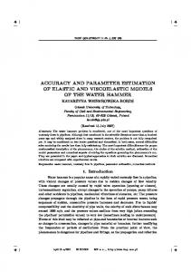
e2

en

r1

r2

rn

Figure 1: Rheological model of the viscoelastic behavior with 𝑛 Maxwell elements.

The applied methods and their advantages are shown with respect to a material model according to the work of Scheffer [22]. In order to focus on the process itself the data bases for the identification are not the original experimental values, where signal noise and statistics play an important role. Moreover, it is not finally sure whether the resulting parameters in the work of Scheffer [22] represent the optimal set since the model is of high complexity in order to describe a nonlinear viscoelastic material behavior depending on the deformation velocity. Hence, for this article the model with the already identified parameters is taken as the reference and the parameters are reidentified. As the main advantage the exact values of the parameters are known and it can be proven if the proposed methods find this exact solution of the problem. Organization of the Article. In Section 2 the theoretical aspects concerning the material description and the resulting constitutive equations are discussed. In Section 3 the problem of parameter identification as an inverse problem is addressed. Section 4 verifies the usage of the proposed methods by showing theoretical results for simplified material models as well as by reconstructing given material parameters. The paper is concluded with a summary and an outline of future research in Section 5.

2. Mathematical Model A new approach for identifying material parameters is discussed here. There are many viscoelastic materials, and different models exist to characterize them fully. To test the approach, the following model is used: It is inspired by real life experiments and is based on a rheological model, where a spring is positioned in parallel to 𝑗 = 1, . . . , 𝑛 Maxwell elements. Each of the Maxwell elements consists of a spring connected in series to a dashpot; compare, Figure 1 (Figure 1 is reprinted by permission from Springer Customer Service Centre GmbH: [23]). The single spring represents the equilibrium stiffness, whereas the Maxwell elements describe the viscoelastic effects. Even the 3-parameter model consisting of a spring and one Maxwell element in parallel shows the main viscoelastic effects, namely, relaxation and creep. The mathematical structure of this rheological model forms the basis for the nonlinear and three-dimensional formulation used in the following investigations.

Mathematical Problems in Engineering

3

1.8

to the Clausius-Planck inequality for isothermal processes with respect to the argumentation of Coleman and Noll [26] leading to

1.6 1.4

T11 (N/mＧ2 )

1.2

T = −𝑝I + 2𝜌0 B ⋅

1.0 0.8

𝜕B

𝑛

𝑗 𝜕𝜓neq

𝑗=1

𝜕B𝑒

+ ∑ 2𝜌0 B𝑗𝑒 ⋅

𝑗

(4)

with 𝑝 as the Lagrangian multiplicator representing the incompressibility of the material. Evaluating (4) for the chosen free energy function results in

0.6 0.4 0.2

2

0.0

T = −𝑝I + 2 [𝑐10 + 2𝑐20 (𝐼B − 3) + 3𝑐30 (𝐼B − 3) ] B

−0.2 −0.4 0.75

𝜕𝜓eq

(5)

4

1.00

1.25

1.50  1 (-)

1.75

2.00

2.25

+ ∑ 2𝑐10𝑗 B𝑗𝑒 . 𝑗=1

The time-dependent behavior of the Maxwell elements is described by the evolution equations

Experiment Simulation

Figure 2: Typical stress-strain diagram.

4 1 𝑗 𝑗 −1 𝑗 Ċ 𝑖 = [C − tr (C ⋅ (C𝑖 ) ) C𝑖 ] 𝑟𝑗 3

The basic elasticity is given as the equilibrium response and serves as the basis for the further material model. A basic elasticity curve for elastomers often shows stiffening for larger deformation values resulting in the typical S-shaped stressstrain curve. This shape of the stress-strain correlation can be monitored by a Yeoh model [24] with the free energy function: 2

3

𝜌0 𝜓eq (𝐼B ) = 𝑐10 (𝐼B − 3) + 𝑐20 (𝐼B − 3) + 𝑐30 (𝐼B − 3) , (1)

with the first invariant 𝐼B = trB in the third order. Here B = F ⋅ F𝑇 is the left Cauchy-Green deformation tensor and F is the deformation gradient. The higher-order approach can monitor the S-shaped upturn of the stress-strain correlation for bigger strains. Figure 2 shows a typical stress-strain diagram for a carbon black filled rubber sample for the basic elasticity as investigated in [23]. To cover the different time ranges in the relaxation behavior, four Maxwell elements are used. The viscoelastic behavior can be captured by the easiest neo-Hookean approach for the springs in the Maxwell elements. This leads to the free energy contribution: 4

𝜌0 𝜓neq (𝐼B ) = ∑ 𝑐10𝑗 (𝐼B𝑗𝑒 − 3) .

(2)

𝑗=1

The total free energy is given by the sum of (1) and (2): 𝜌0 𝜓 = 𝜌0 𝜓eq + 𝜌0 𝜓neq .

(3)

In the equations, B describes the deformation in the single equilibrium spring and B𝑗𝑒 = F𝑗𝑒 ⋅ (F𝑗𝑒 )𝑇 represents the elastic deformation in the 𝑗th Maxwell element. The underlying multiplicative split of the deformation gradient F = F𝑒 ⋅ F𝑖 was well established in finite strain theories of plasticity or viscoelasticity; compare, for example, [25]. The Cauchy stress T is obtained from the free energy functions according

𝑗

𝑗

𝑗 = 1, . . . , 4 𝑗

(6)

for the inelastic deformation C𝑖 = (F𝑖 )𝑇 ⋅ F𝑖 in the dashpot 𝑗 of the 𝑗th Maxwell element; see [27]. Ċ 𝑖 are the material time rates of the inelastic right Cauchy-Green deformation tensors 𝑗 C𝑖 . The parameters 𝑟𝑗 in the evolution equation stand for the so-called relaxation time. They have to be chosen according to observation from relaxation tests. Usually different relaxation processes take place in a black carbon filled rubber. While the fastest process is triggered by the loading time 𝑡max , the slowest process is governed by the total time of observation 𝑏max . For simplicity the relaxation times of the model are equally distributed with this time interval on a logarithmic scale. Figure 3 shows the theoretical strain that a material experiences during the relaxation experiments and its stress answer. In the experiments, the stretch values 𝜆, which are the ratio of current length 𝑙 to initial length 𝑙0 , are steadily increased until the maximum values 𝜆 max are reached and are then held there. The time when this maximum is reached is denoted by 𝑡max . While in an idealised relaxation test the loading is applied instantaneously, in real experiments 𝑡max is mainly governed by the maximum speed of the experimental device. Furthermore, the stop time of the experiments is denoted by 𝑏max . In the stress answer of the material an increase is noticed until 𝑡max where the maximum is reached. From then on, the stress tends towards the basic stress value 𝑇eq while the deformation does not change. This process is called relaxation. The relaxation times were chosen in such a way that the physical restrictions in the experiments are preserved. On one side the maximal device velocity that is used in the experiments gives a lower bound for the smallest observable relaxation time. On the other side the time span of the experiment determines the longest relaxation time. In order to cover a broad interval, the relaxation times are set in a range of multiple powers of ten as seen in Table 1. It also shows the identified material parameters from the aforementioned

4

Mathematical Problems in Engineering

 (t)

T (t)

 Ｇ；Ｒ

tＧ；Ｒ

T？Ｋ

bＧ；Ｒ

tＧ；Ｒ

bＧ；Ｒ

t

t

(a)

(b)

Figure 3: Relaxation test. Table 1: Used parameters. 𝑐10 [MPa] 0.200

𝑐20 [MPa] −0.052

𝑐30 [MPa] 0.017

𝑐101 [MPa] 0.009

𝑐102 [MPa] 0.1045

experiments performed on a black carbon filled rubber [23]. They are mechanically meaningful and can be used to test the here proposed reconstruction methods. Due to the complexity of the model the identification of its parameters is far from being trivial. In general, an inverse problem is formulated in such a way that the parameters are chosen by minimization of the error between data and experiments.

3. Regularization Methods If we neglect modeling errors, then the exact parameters and those which have been predicted by solving the inverse identification problem, coincide. This leads to the equation 𝑏 (𝑡𝑖 ) = 𝜑 (𝑡𝑖 ; 𝑐1 , . . . , 𝑐𝑛 ) ,

(7)

where 𝑏𝑖 = 𝑏(𝑡𝑖 ) are the measurements at 𝑚 different time steps 𝑡𝑖 , 𝜑 the approximative model, and 𝑐1 , . . . , 𝑐𝑛 the unknown (exact) material parameters. Due to inevitable errors in the experiments and the fact that the model is unable to describe the real process exactly, the residue V𝑖 can only be approximated by 𝑐1 , . . . , 𝑐𝑛 ) − 𝑏𝑖 , 𝑖 = 1, . . . , 𝑚. V𝑖 = 𝜑 (𝑡𝑖 ; ⏟⏟⏟⏟⏟⏟⏟⏟⏟⏟⏟⏟⏟⏟⏟

(8)

c

With the goal in mind to minimize the residues with respect to the model parameters, the V𝑖 and 𝑐𝑗 are unified into vectors k and c, respectively, and one obtains the minimization problem min𝑛 c∈R

𝑚 1 1 ‖k‖22 = min𝑛 ∑V𝑖2 . 2 2 c∈R 𝑗=1

(9)

𝑐103 [MPa] 0.065

𝑐104 [MPa] 3.382

𝑟1 [s] 0.1

𝑟2 [s] 1

𝑟3 [s] 10

𝑟4 [s] 100

Due to the nature of the presented constitutive model (5), the equations are simplified to linear ones with respect to c with a common form. This leads for 𝑚 values of the stretch 𝜆 𝑘 , 𝑘 = 1, . . . , 𝑚 to 𝑇 (𝜆 𝑘 ) = 𝑎1 (𝜆 𝑘 ) 𝑐1 + ⋅ ⋅ ⋅ + 𝑎𝑛 (𝜆 𝑘 ) 𝑐𝑛 .

(10)

For different values of the stretch 𝜆 𝑘 , which explicitly depends on time, we obtain the stress as a linear combination of the coefficients 𝑎𝑗 (𝜆 𝑘 ) determined from the model equations and the material parameters 𝑐𝑗 . The coefficients 𝑎𝑗 (𝜆 𝑘 ) are given by (5) and are united into a vector a𝑘 : a𝑘 = (𝑎1 (𝜆 𝑘 ) , 𝑎2 (𝜆 𝑘 ) , . . . , 𝑎𝑛 (𝜆 𝑘 )) ∈ R𝑛 .

(11)

For rate-dependent material behavior, the stress and the coefficients in a𝑘 have explicit additional dependency on the inelastic stretch 𝜆 𝑖 . In the following we do not investigate data measured in real experiments but for simplicity we treat the so-called problem of parameter reidentification. Therefore, the used data are not derived from actual experiments but are obtained by the stress-strain relationship given by the constitutive equations and a set of known parameters; compare Table 1. To further simulate errors in the measurement process, a perturbation by white additive Gaussian noise is added to the simulated stress vector, which leads to 󵄩 󵄩󵄩 󵄩󵄩b − b𝛿 󵄩󵄩󵄩 < 𝛿, (12) 󵄩 󵄩 where b is the simulated stress vector and b𝛿 the perturbed one. Here, 𝛿 measures the deviation between the two vectors and is called noise level. From here on out we use b𝛿 as (simulated) input data.

Mathematical Problems in Engineering

5

The vectors a𝑘 are collected to build the rows of a single matrix A: 𝑇

A = (a1 , a2 , . . . , a𝑚 ) ∈ Mat𝑚,𝑛 (R) .

(13)

Thus we have A = (𝑎𝑘𝑗 ) with 𝑎𝑘𝑗 fl 𝑎𝑗 (𝜆 𝑘 ). With the vector c containing material parameters and b𝛿 containing stress values 𝑇, one obtains the following minimization problem: 1 󵄩󵄩 󵄩2 󵄩󵄩Ac − b𝛿 󵄩󵄩󵄩 󵄩 󵄩 2

min𝑛 c∈R

1 󵄩󵄩 󵄩2 󵄩󵄩Ac − b𝛿 󵄩󵄩󵄩 󵄩 2󵄩

(15)

and its derivatives ∇𝐹 (c) = A𝑇 Ac − A𝑇b𝛿 ,

(16)

H𝐹 (c) = A𝑇 A, 𝑇

it can be shown that the 𝑛 × 𝑛-matrix H𝐹 = A A is symmetric and positive definite, if A has full rank, so that the extremum of ∇𝐹 is an absolute minimum. Setting ∇𝐹 = 0 leads to the so-called normal equation 𝑇

∗

𝑇 𝛿

A Ac = A b .

(17)

This equation has a unique solution, if rang(A) = 𝑛. This can be realized by using a sufficient number of samples. The solution of (17) is then given as c∗ = A+ b𝛿 ,

(18)

where A+ is defined as the pseudoinverse +

𝑇

−1

𝑇

A = (A A) A .

(19)

The difficulties that may arise when computing the inverse of a matrix should be mentioned here. Explicitly, one should consider the condition of the problem. It tells how much the obtained solution deviates from the real one if the input data is perturbed. In general, a problem is called well-conditioned when small errors in the input data only generate small errors in the solution. On the other hand, an ill-conditioned problem gives rise to big errors in the solution for small perturbation of the data. For linear problems, the condition number 𝜅(A) of a matrix A can be calculated with the help of the singular values by 𝜅 (A) =

𝜎max (A) 𝜎min (A)

min𝑛 c∈R

(14)

with b𝛿 = (𝑏1𝛿 , . . . , 𝑏𝑚𝛿 )𝑇 . The minimization problem is differentiable due to the Euclidean norm and can therefore be solved by setting the first derivative equal to zero as a necessary condition. By defining a function 𝐹 (c) =

To compensate for the measurement errors which possibly lead to the bad condition of A+ , we propose a regularization scheme that is based on the Tikhonov-Phillips method; see, for example, [18]. A penalty term is added to the minimization problem (14) such that the norm of the solution vector ‖c‖ is to be as small as possible. This leads to the minimization problem

(20)

with 𝜎max and 𝜎min being the largest and smallest singular value, respectively.

1 󵄩󵄩 󵄩2 𝛾 󵄩󵄩Ac − b𝛿 󵄩󵄩󵄩 + ‖c‖2 󵄩 2󵄩 2

(21)

with the regularization parameter 𝛾 ≥ 0. By differentiating with respect to c, we see that any solution c∗ has to satisfy the shifted normal equation (A𝑇 A + 𝛾I) c∗ = A𝑇 b𝛿 .

(22)

Since the matrix A𝑇A + 𝛾I is invertible, there exists a unique solution of (21) for all 𝛾 > 0. The nature of the given problem encourages an additional penalty term. The second parameter of the basic parameters, that is, 𝑐20 , has to be negative due to the characteristic shape of the stress-strain relation. Positive values of 𝑐20 are therefore penalized such that (21) becomes min𝑛 c∈R

1 󵄩󵄩 󵄩2 𝛾 󵄩󵄩Ac − b𝛿 󵄩󵄩󵄩 + ‖c‖2 + 𝛽𝑐20 , 󵄩 󵄩 2 2

(23)

where 𝛽 > 0 denotes a further regularization parameter. The optimality condition for the minimizing c∗ is then given as (A𝑇 A + 𝛾I) c∗ = A𝑇 b𝛿 − 𝛽e2

(24)

with (e2 )𝑗 = 1 for 𝑗 = 2 and 0 otherwise. The multiparameter setting as in (23) is closely related to elastic-net regularization which originates from statistics, see [28], and has been analyzed in [29].

4. Virtual Experiments In the virtual experiments the three aforementioned regularization methods are used. Method 1 is the unregularized normal equation (17), method 2 is the regularized Tikhonov equation (22), and method 3 is given by (24), which adds an extra penalty term to guarantee the negativity of the basic elastic parameter 𝑐20 . Furthermore we divide the experiments into three categories depending on the characteristics of the reconstructed parameters. At first, set 1 with the basic elastic parameters 𝑐10 , 𝑐20 , and 𝑐30 is reconstructed. Subsequently the viscoelastic parameter set 2 with 𝑐101 , 𝑐102 , 𝑐103 , and 𝑐104 is computed using the elastic parameters as a priori information. Lastly, all parameters from the previous sets are put together in set 3 and reconstructed at the same time. As long as viscoelastic parameters are involved, we additionally consider a simplified model to work out additional dependence on the used relaxation times. To compare the different reconstruction methods, an error measurement is introduced. The reconstruction error 𝜎 is the normalized difference between the vector c0 with the identified parameters from Table 1 and the vector c with

6

Mathematical Problems in Engineering 240

Table 2: Reconstruction of parameter set 1 with regularization in dependence of 𝜆 max (𝛾 = 0.5, 𝛽 = 0.1).

220

𝜆 2 1.5

200 Condition number 

180 160

𝑐10 [MPa] 0.1960 0.2080

𝑐20 [MPa] −0.0495 −0.0777

𝑐30 [MPa] 0.0164 0.0410

140 120 100 80 60 40 20 0

5

10

15

20

25

30

35

40

45

50

Data points m =2

 = 1.25  = 1.5  = 1.75

Figure 4: Condition numbers for parameter set 1 in dependence of 𝜆 max .

the newly reconstructed parameters with this approach in the Euclidean norm; that is, 󵄩󵄩 󵄩 󵄩c − c󵄩󵄩 (25) 𝜎 = 󵄩 󵄩󵄩0 󵄩󵄩 󵄩 . 󵄩󵄩c0 󵄩󵄩 In our tests we choose a noise level 𝛿 varying in the range of [0, 0.7] to display the results of our methods depending on the noise level. The value 𝛿 = 0.0 corresponds to exact (simulated) data. We perform 100 realizations for every value of 𝛿 which are averaged afterwards in order to reduce fluctuations in 𝜎 due to the added random noise. Note that the type of material being tested may also affect the noise level. 4.1. Reconstruction of Parameter Set 1: Reconstructing the Basic Elasticity Parameters. At first the basic elastic parameters are reconstructed. As our investigations are based on uniaxial tension tests, the tensorial constitutive equation is reduced to the scalar-valued stress-response as a function of the stretch: 𝑇eq = [2𝑐10 + 4𝑐20 (𝜆2 +

2 − 3) 𝜆

2 2 1 + 6𝑐30 (𝜆 + − 3) ] (𝜆2 − ) . 𝜆 𝜆

(26)

2

By evaluating (26) 𝑚 times, one obtains the linear system of equations Ac = b

𝛿

(27)

of the maximum stretch 𝜆 max . For a doubled probe length 𝜆 max = 2, the condition number 𝜅 decays rapidly if more data points are used until it is almost constant with 𝑚 ≥ 20. In the other cases, similar observations can be made and therefore 𝑚 = 20 is constant for further considerations. Since 𝑛 = 3 and the total time of observation 𝑏max are fixed, it is quite natural that the condition of A saturates for growing 𝑚 at a certain level. The reason is that for a fixed number of columns 𝑛 and fixed observation time 𝑏max we do not expect that 𝜎max (A) → +∞ or 𝜎min (A) → 0 as 𝑚 → ∞. Moreover, we have that rank(A) = 3, independently of 𝑚, and thus there are at most 3 singular values which are not identical 0. We discuss now the regularization for two different values of the stretch, namely, 𝜆 max = 2 and 𝜆 max = 1.5. The results are illustrated in Figure 5. A regularization for a material with double the length and 𝜆 max = 2 does not seem to be necessary. Even the unregularized reconstruction gives reasonable low errors 𝜎. For small derivations from the original stress vector b, the results get even worse. For the smaller strain value the advantages of the regularization become more pronounced. The reconstruction error barely reaches a value of 𝜎 = 0.4 in method 2, whereas we face larger errors for the unregularized reconstruction. Additionally the advantages of the second regularization term with 𝛽 in method 3 can be shown. For 𝜆 max = 1.5 the relative error 𝜎 may be small in method 2, but by a closer look it is revealed that 50 percent of the values of 𝑐20 are positive and therefore the reconstruction is not satisfying. With the additional regularization term, the percentage of positive values can be reduced to 4 percent and the relative error is even further reduced. For 𝜆 max = 2 the number of positive values for 𝑐20 is also reduced by half in method 3. The quantitative reconstruction of the parameters is shown in Table 2 for 𝛿 = 0.5. For both choices of 𝜆 max a sufficient reconstruction is possible with a worse result in the smaller interval up to 𝜆 max = 1.5. 4.2. Reconstruction of Parameter Set 2: Incorporating the Viscoelastic Parameters. The model is extended by incorporating viscoelastic parameters. The constitutive equation has the following form: 𝑇 2 2 2 1 = [2𝑐10 + 4𝑐20 (𝜆2 + − 3) + 6𝑐30 (𝜆2 + − 3) ] (𝜆2 − ) 𝜆 𝜆 𝜆 ⏟⏟⏟⏟⏟⏟⏟⏟⏟⏟⏟⏟⏟⏟⏟⏟⏟⏟⏟⏟⏟⏟⏟⏟⏟⏟⏟⏟⏟⏟⏟⏟⏟⏟⏟⏟⏟⏟⏟⏟⏟⏟⏟⏟⏟⏟⏟⏟⏟⏟⏟⏟⏟⏟⏟⏟⏟⏟⏟⏟⏟⏟⏟⏟⏟⏟⏟⏟⏟⏟⏟⏟⏟⏟⏟⏟⏟⏟⏟⏟⏟⏟⏟⏟⏟⏟⏟⏟⏟⏟⏟⏟⏟⏟⏟⏟⏟⏟⏟⏟⏟⏟⏟⏟⏟⏟⏟⏟⏟⏟⏟⏟⏟ 𝑇eq

𝑇

with A ∈ Mat𝑚,3 (R), c = (𝑐10 , 𝑐20 , 𝑐30 ) , and the perturbed stress vector b𝛿 ∈ R𝑚 . In a first step, the condition of matrix A has to be considered. Figure 4 shows the condition for different values

4

2

𝑗 𝜆𝑖

𝜆 + ∑ 2𝑐10𝑗 ( − ). 𝑗 2 𝜆 𝑗=1 (𝜆 ) 𝑖 ⏟⏟⏟⏟⏟⏟⏟⏟⏟⏟⏟⏟⏟⏟⏟⏟⏟⏟⏟⏟⏟⏟⏟⏟⏟⏟⏟⏟⏟⏟⏟⏟⏟⏟⏟⏟⏟⏟⏟⏟⏟⏟⏟⏟⏟ 𝑇neq

(28)

0.28 0.26 0.24 0.22 0.2 0.18 0.16 0.14 0.12 0.1 0.08 0.06 0.04 0.02 0

7

1.6 1.4 1.2 Parameter error 

Parameter error 

Mathematical Problems in Engineering

1 0.8 0.6 0.4 0.2

0 0.05 0.1 0.15 0.2 0.25 0.3 0.35 0.4 0.45 0.5 0.55 0.6 0.65 0.7 Noise level 

0

0 0.05 0.1 0.15 0.2 0.25 0.3 0.35 0.4 0.45 0.5 0.55 0.6 0.65 0.7 Noise level  Method 1 Method 2 with  = 0.5 Method 3 with  = 0.5,  = 0.1

Method 1 Method 2 with  = 0.5 Method 3 with  = 0.5,  = 0.1 (a) 𝜆 max = 2

(b) 𝜆 max = 1.5

Figure 5: Reconstruction of parameter set 1 in dependence of 𝜆 max .

Table 3: Condition numbers for the simplified model. 𝑚 15 20 25 30

𝑡max [s] 0.01 5.7297 8.1053 5.5608 5.9307

0.1 7.1685 6.5995 7.0681 6.6409

1 12.0725 12.9576 13.0173 12.3669

10 19.2962 19.5821 19.7707 19.1556

Table 4: Reconstruction of the viscoelasticity parameters 𝑐101 and 𝑐102 . (a) 𝑐101 = 1, 𝑐102 = 1, 𝛾 = 0.5

𝑡max [s] 10 > 𝑟2 1 = 𝑟2 0.1 = 𝑟1 0.01 < 𝑟1

𝑐101 [MPa] 0.0163 0.1541 0.6251 0.9175

𝑐102 [MPa] 0.1351 0.9227 1.0661 1.0349

(b) 𝑐101 = 1, 𝑐102 = 1, 𝛾 = 1.5

As the identified basic elastic parameters are kept fixed in this step we only consider the viscoelastic parameter reconstruction and the data is solely produced by 𝑇neq . In the viscoelastic case the data points have to be distributed logarithmically on the interval [0, 𝑏max ], such that more weight is put onto the loading process of the deformation than the relaxation process. 4.2.1. Simplified Parameter Reconstruction. Due to the more complex material behavior, the importance of the relaxation times of the different Maxwell elements has to be considered first. To test the influence of the relaxation times on the reconstruction, simulated data with a simplified material model in mind have to be constructed. Only two Maxwell elements with relaxation times 𝑟1 = 1 s and 𝑟2 = 10 s are used. With this simplified model the influence of the different parameters can be studied. The condition only differs slightly if the values for 𝜆 max , 𝑏max or the number of data points 𝑚 is changed. On the other side, different values for 𝑡max have a big effect on the condition as can be seen in Table 3. Physically, for a given 𝜆 max the parameter 𝑡max stays in direct relationship to the deformation

𝑡max [s] 10 > 𝑟2 1 = 𝑟2 0.1 = 𝑟1 0.01 < 𝑟1

𝑐101 [MPa] 0.0058 0.0993 0.4209 0.8091

𝑐102 [MPa] 0.0477 0.7099 1.0659 1.0604

velocity of the material. Slower deformation rates correspond to greater values of 𝑡max , whereas small values belong to faster deformations. Table 4 shows the reconstruction of the simplified model if the parameters 𝑐101 , 𝑐102 are chosen as 1 MPa. A bigger value for the choice of the regularization parameter 𝛾 penalizes the norm of c too much and should therefore be chosen accordingly. For further investigations a value of 𝛾 = 0.5 is chosen. It can be recognized that the reconstructed value of parameter 𝑐10𝑗 is within a tolerance as soon as 𝑡max is smaller than 𝑟𝑗 . Further observations can be made if the parameters are chosen similar to the relaxation times in decades. Table 5 shows the reconstruction for 𝑐101 = 1 MPa and 𝑐102 = 10 MPa

8

Mathematical Problems in Engineering

Table 5: Reconstruction of the viscoelasticity parameters with different values. (a) 𝑐101 = 1, 𝑐102 = 10

𝑡max [s]

𝑐101 [MPa]

𝑐102 [MPa]

10 > 𝑟2 1 = 𝑟2 0.1 = 𝑟1

0.1473 1.0612 1.5237

1.2316 8.3039 9.7804

0.01 < 𝑟1

1.3703

9.9070

(b) 𝑐101 = 10, 𝑐102 = 1

𝑡max [s]

𝑐101 [MPa]

𝑐102 [MPa]

10 > 𝑟2 1 = 𝑟2

0.0353 0.5581

0.2651 1.8267

0.1 = 𝑟1 0.01 < 𝑟1

5.3249 8.7564

1.9583 1.4773

160

Condition numbers 

140

Table 6: Reconstruction of the viscoelasticity parameters in dependence of 𝑡max . 𝑡max [s] 0.01 1

𝑐101 [MPa] 0.0492 0.0116

𝑐102 [MPa] 0.0447 −0.3493

𝑐103 [MPa] 0.1408 0.1814

𝑐104 [MPa] 3.3396 3.3289

at the same time a relatively fast deformation rate. These rates cannot be obtained in current experiments. Therefore a more realistic value of 𝑡max = 1 s is also tested. In this case, regularization leads to better results again. The regularized reconstruction error never exceeds 𝜎 = 0.06, whereas the unregularized one increases for bigger noise levels. The quantitative reconstruction in Table 6 shows the characteristics of the simplified tests. For 𝑡max = 0.01 s, the parameter 𝑐104 is reconstructed well, whereas the others show overshooting values. The smaller the relaxation time, the bigger the error gets. For 𝑡max = 1 s, which is closer to real experiments, the parameters get reconstructed appropriately, but a negative value for 𝑐102 is observed. This behavior is according to the choice of 𝑡max as 𝑟2 > 𝑡max .

120 100 80 60 40 20 0

0

5

10

15

20

25

30

35

40

45

50

Data points m tＧ；Ｒ = 0.01 s tＧ；Ｒ = 1 s

Figure 6: Condition numbers for parameter set 2 in dependence of 𝑡max .

and vice versa. In addition to the prior observations, it is also noted that the reconstruction of the parameters belonging to small relaxation times is not as good as the ones belonging to the bigger relaxation times. 4.2.2. Original Parameter Reconstruction. For the reconstruction of the exact parameters of the original model, the condition can be observed in Figure 6 for different values of 𝑡max . The number of samples is chosen as 𝑚 = 15 in these experiments. The actual reconstruction is shown in Figure 7 with different values for 𝑡max . According to earlier observation the regularization is not necessary for 𝑡max = 0.01 s. The error for the unregularized solution is as low as the error for the regularized one. The reconstruction error 𝜎 is small in either method though. A small 𝑡max means

4.3. Reconstruction of Parameter Set 3: All-at-Once Computation of the Parameters. At last, the question arises if it is necessary to do the time-consuming identification of basic elasticity parameters beforehand. In case of highly filled rubbers the relaxation of the specimen can be observed for very long times. Therefore, the experiments are really timeconsuming if the basic elasticity should be observed; see, for example [22]. In this case the sequential identification presented above is not possible. A simultaneous identification by means of our methods is proposed in the next step. For the following experiments the data vector b𝛿 consists of values of (28). The parameters 𝜆 max = 2 and 𝑏max = 500 s are fixed. The regularization parameters are chosen as 𝛾 = 0.5 and 𝛽 = 0.1. 4.3.1. Simplified Parameter Reconstruction. In the first step the simplified model from Section 4.2.1 is extended. Next to the parameters 𝑐101 and 𝑐102 for the viscoelasticity, the basic elasticity parameters 𝑐10 , 𝑐20 , and 𝑐30 can be chosen freely. The condition of the 𝑚 × 5-matrix is shown in Table 7. For values of 𝑡max as 0.1 s or 1 s, we still obtain a reasonable condition whereas we observe an exponentially increasing condition number as 𝑡max → 0. To restrict the workload on the experimentator, the number of samples is chosen as 𝑚 = 30. The values of the exact parameters have been chosen as in Table 8. Table 9 shows reconstructions for different values of 𝑡max . It has to be distinguished between two types of parameters. On the one hand the viscoelastic parameters show the same patterns with respect to 𝑡max and the relaxation times 𝑟𝑗 as before. On the other hand an insufficient reconstruction of the basic parameters for a small choice of 𝑡max can be observed. Therefore the choice for 𝑡max builds a contradiction. One explanation can be found in the unusually high condition in the range of 1018 .

Mathematical Problems in Engineering

9

0.06

0.45

0.05

0.4

0.05

0.35 Parameter error 

Parameter error 

0.04 0.04 0.03 0.03 0.02 0.02

0.25 0.2 0.15 0.1

0.01

0.05

0.01 0

0.3

0 0.05 0.1 0.15 0.2 0.25 0.3 0.35 0.4 0.45 0.5 0.55 0.6 0.65 0.7 Noise level  Method 1 Method 2 with  = 0.5

0

0 0.05 0.1 0.15 0.2 0.25 0.3 0.35 0.4 0.45 0.5 0.55 0.6 0.65 0.7 Noise level  Method 1 Method 2 with  = 0.5

(a) 𝑡max = 0.01 s

(b) 𝑡max = 1 s

Figure 7: Reconstruction of parameter set 2 in dependence of 𝑡max .

Table 7: Condition numbers for the simplified model. 𝑡max [s]

𝑚

0.01 9.24 ⋅ 1018 8.49 ⋅ 1018 4.82 ⋅ 1018 2.35 ⋅ 1019 6.94 ⋅ 1019

15 20 25 30 35

0.1 2.684 ⋅ 103 2.77 ⋅ 103 1.83 ⋅ 103 1.74 ⋅ 103 1.52 ⋅ 103

Table 8: Values of the exact parameters in the simplified model. 𝑐10 [MPa] 1

𝑐20 [MPa] −1

𝑐30 [MPa] 1

𝑐101 [MPa] 1

𝑐102 [MPa] 1

Furthermore, similar observations as before can be made if one of the viscoelastic parameters gets multiplied by 10, as seen in Table 10. By the Tikhonov regularization a simultaneous reconstruction of all parameters is performed since the minimization of (23) averages the norm of the penalty term. This leads to over- and underestimations in the reconstructed solution c. A possible remedy could be a separate regularization with ceq containing the basic elasticity parameters and cneq containing the viscoelasticity parameters. 4.3.2. Original Parameter Reconstruction. In a last step the quality of the reconstruction of the actual parameters is tested. The range in which the condition lies does not change. For 𝑡max = 0.01 s the values lie in the range of 1018 going afterwards down to 103 for larger values of 𝑡max . Due to

1 2.99 ⋅ 103 3.08 ⋅ 103 3.35 ⋅ 103 3.09 ⋅ 103 2.95 ⋅ 103

10 1.85 ⋅ 104 1.77 ⋅ 104 1.76 ⋅ 104 1.65 ⋅ 104 1.71 ⋅ 104

this ill-posed problem a reasonable reconstruction without regularization is impossible for 𝑡max = 0.01. With our two methods of regularization, however, sufficient results with an error measurement 𝜎 < 0.12 are reached. Figure 8 shows the reconstruction of the parameter for 𝑡max = 1 s. Without regularization the error is increasing for higher values of 𝛿. The regularized solutions never exceed 𝜎 = 0.04. The importance of the regularization parameter 𝛽 is again shown. Even though the error is minimally larger for method 3, only 10 percent of the values for 𝑐20 are positive whereas we have 53 percent positive values in method 2. Table 11 shows the actual reconstructed values for two values of 𝑡max . We see the contradicting influence of 𝑡max . For a small value we reconstruct the viscoelastic parameters well but suffer a massive undershoot for the basic parameter 𝑐10 . For the bigger value of 𝑡max the basic elasticity parameters can be reconstructed while the viscoelastic ones are slightly undershot. Remark 1. Knowing the ground truth as in our simulations the regularization parameters 𝛾 and 𝛽 can easily be adjusted by trial and error. Of course, this is no longer possible in case

10

Mathematical Problems in Engineering Table 9: Reconstruction of parameters in the simplified model.

𝑡max [s] 10 > 𝑟2 1 = 𝑟2 0.1 = 𝑟1 0.01 < 𝑟1

𝑐10 [MPa] 0.9470 1.0030 0.9648 0.0705

𝑐20 [MPa] −0.9166 −0.9247 −0.8849 0.0346

𝑐30 [MPa] 0.9766 0.9821 0.9722 0.7402

𝑐101 [MPa] 0.0300 0.2310 0.6960 0.9455

𝑐102 [MPa] 0.2448 0.8682 1.0135 1.0240

Table 10: Reconstruction of parameters with different values. (a) 𝑐101 = 1, 𝑐102 = 10

𝑡max [s]

𝑐10 [MPa]

𝑐20 [MPa]

𝑐30 [MPa]

𝑐101 [MPa]

𝑐102 [MPa]

10 > 𝑟2

1.7450

−1.3238

1.0459

0.1638

1.1793 4.8626

1 = 𝑟2

3.4953

−1.5015

0.9680

1.1327

0.1 > 𝑟1

0.9354

−0.7622

0.9348

1.2218

9.8011

0.01 < 𝑟1

0.0703

0.0361

0.7406

1.2255

9.9818

(b) 𝑐101 = 10, 𝑐102 = 1

𝑡max [s]

𝑐10 [MPa]

𝑐20 [MPa]

𝑐30 [MPa]

𝑐101 [MPa]

𝑐102 [MPa]

10 > 𝑟2

1.0231

−0.9556

0.9832

0.0570

0.3853 1.7708

1.3213

−1.1901

1.0440

0.8043

0.1 = 𝑟1

3.5345

−1.6759

1.0208

3.1867

1.5396

0.01 < 𝑟1

0.0961

0.0264

0.7397

9.1108

1.3099

Parameter error 

1 = 𝑟2

0.3 0.28 0.26 0.24 0.22 0.2 0.18 0.16 0.14 0.12 0.1 0.08 0.06 0.04 0.02 0

where c∗𝑘 solves (24) with parameters 𝛾𝑘 , 𝛽𝑘 . Finally we set 𝛾 fl 𝛾𝑘∗ , 𝛽 fl 𝛽𝑘∗ . In this way it is guaranteed that the noise in the residuum is of the same order as the noise in the data. Heuristic methods for choosing 𝛾, 𝛽 depending only on the measured data b𝛿 , which is of relevance if the noise level 𝛿 is not known and cannot be estimated, are the L-curve criterion or generalized cross validation. We refer the interested reader to the standard textbook [18] for more details on parameter choice rules.

5. Conclusion

0 0.05 0.1 0.15 0.2 0.25 0.3 0.35 0.4 0.45 0.5 0.55 0.6 0.65 0.7 Noise level  Method 1 Method 2 with  = 0.5 Method 3 with  = 0.5,  = 0.1

Figure 8: Reconstruction of parameter set 3 with 𝑡max = 1 s.

of real, measured data. The most popular parameter choice rule in this case is Morozov’s discrepancy principle, which works as follows: Choosing null sequences {𝛾𝑘 } and {𝛽𝑘 } as well as a tolerance parameter 𝜏 > 1, we define 𝑘∗ ∈ N by 󵄩 󵄩 𝑘∗ fl min {𝑘 ∈ N : 󵄩󵄩󵄩󵄩Ac∗𝑘 − b𝛿 󵄩󵄩󵄩󵄩 < 𝜏𝛿} ,

(29)

In this article we introduced a method for identifying material parameters from constitutive equations by means of a Tikhonov regularization. An extra penalty term which is directly inspired from the stress-strain relationship for the chosen material is added to expect reasonable results. Overall, this method ensures a fast and convenient way to identify both the basic elastic and the viscoelastic parameters at the same time without a time-consuming separated identification. Maybe better reconstruction results can be achieved by using more sophisticated penalty terms. We furthermore mention some shortcomings that are intrinsic to Tikhonov regularization. The first one is the fact that in general 𝜅(A𝑇 A) = 𝜅(A)2 yielding a much worse condition number for A𝑇A, the matrix that appears in systems (22) and (24). A second one must be seen in the determination of appropriate regularization parameters 𝛾 and 𝛽 in case of real data which might be time-consuming and data-dependent. Furthermore, better results can be achieved by correlating the relaxation times with the actual deformation process.

Mathematical Problems in Engineering

11

Table 11: Reconstruction of parameter set 3 in dependence of 𝑡max . 𝑡max [s] 0.01 1

𝑐10 [MPa] 0.0063 0.2130

𝑐20 [MPa] −0.1749 −0.0823

𝑐30 [MPa] 0.0754 0.0273

Finally we note that the methodology is also applicable to alternative constitutive equations like plasticity models. This will be subject of future research.

Conflicts of Interest The authors declare that there are no conflicts of interest regarding the publication of this paper.

References [1] H. Baaser, C. Hopmann, and A. Schobel, “Reformulation of strain invariants at incompressibility,” Archive of Applied Mechanics, vol. 83, no. 2, pp. 273–280, 2013. [2] H. Baaser and R. Noll, Simulation von Elastomerbauteilen: Materialmodelle und Versuche zur Parameterbestimmung, dVM-Tag Elastomere, 2009. [3] H. Baaser, A. Schobel, W. Michaeli, and U. Masberg, “Vergleich von a¨quibiaxialen Pr¨ufst¨anden zur Kalibrierung von Werkstoffmodellen,” KGK. Kautschuk, Gummi, Kunststoffe, vol. 64, no. 5, pp. 20–24, 2011. [4] M. Johlitz and S. Diebels, “Characterisation of a polymer using biaxial tension tests. Part I: hyperelasticity,” Archive of Applied Mechanics, vol. 81, no. 10, pp. 1333–1349, 2011. [5] H. Seibert, T. Scheffer, and S. Diebels, “Biaxial testing of elastomers—experimental setup, measurement and experimental optimisation of specimen’s shape,” Technische Mechanik, vol. 34, no. 2, pp. 72–89, 2014. [6] S. Cooreman, D. Lecompte, H. Sol, J. Vantomme, and D. Debruyne, “Identification of mechanical material behavior through inverse modeling and DIC,” Experimental Mechanics, vol. 48, no. 4, pp. 421–433, 2008. [7] N. Trabelsi, Z. Yosibash, C. Wutte, P. Augat, and S. Eberle, “Patient-specific finite element analysis of the human femura double-blinded biomechanical validation,” Journal of Biomechanics, vol. 44, no. 9, pp. 1666–1672, 2011. [8] S. Klinge, “Inverse analysis for multiphase nonlinear composites with random microstructure,” International Journal for Multiscale Computational Engineering, vol. 10, no. 4, pp. 361–373, 2012. [9] S. Klinge, “Parameter identification for two-phase nonlinear composites,” Computers & Structures, vol. 108, pp. 118–124, 2012. [10] S. Klinge and P. Steinmann, “Inverse analysis for heterogeneous materials and its application to viscoelastic curing polymers,” Computational Mechanics, vol. 55, no. 3, pp. 603–615, 2015. [11] D. Miedzi´nska, T. Niezgoda, and R. Gieleta, “Numerical and experimental aluminum foam microstructure testing with the use of computed tomography,” Computational Materials Science, vol. 64, pp. 90–95, 2012. [12] N. Koprowski-Theiß, Kompressible, viskoelastische Werkstoffe: Experimente, Modellierung und FE-Umsetzung, Dissertation, Universit¨at des Saarlandes, 2011. [13] I. Rechenberg, Evolutionsstrategie ’94, Werkstatt Bionik und Evolutionstechnik, Frommann-Holzboog, 1994.

𝑐101 [MPa] 0.0616 0.0153

𝑐102 [MPa] 0.0239 −0.0156

𝑐103 [MPa] 0.1704 0.2089

𝑐104 [MPa] 3.3067 3.2952

[14] R. M. Lewis and V. Torczon, “Pattern search algorithms for bound constrained minimization,” SIAM Journal on Optimization, vol. 9, no. 4, pp. 1082–1099, 1999. [15] V. Torczon, “On the convergence of pattern search algorithms,” SIAM Journal on Optimization, vol. 7, no. 1, pp. 1–25, 1997. [16] J. A. Nelder and R. Mead, “A simplex method for function minimization,” The Computer Journal, vol. 7, no. 4, pp. 308–313, 1965. [17] A. K. Louis, Inverse und schlecht gestellte Probleme, Teubner, Stuttgart, Germany, 1989. [18] H. W. Engl, M. Hanke, and A. Neubauer, Regularization of Inverse Problems, Mathematics and Its Applications, Kluwer Academic Publishers, Dordrecht, The Netherlands, 1996. [19] A. Rieder, Keine Probleme mit Inversen Problemen, Vieweg, Wiesbaden, Germany, 2003. [20] T. Schuster, B. Kaltenbacher, B. Hofmann, and K. S. Kazimierski, Regularization Methods in Banach Spaces, De Gruyter, 2012. [21] A. N. Tikhonov and V. Y. Arsenin, Solutions of Ill-Posed Problems, John Wiley & Sons, New York, NY, USA, 1977. [22] T. Scheffer, Charakterisierung des nichtlinear-viskoelatischen Materialverhaltens gef¨ullter Elastomere, Universit¨at des Saarlandes, 2016. [23] T. Scheffer, H. Seibert, and S. Diebels, “Optimisation of a pretreatment method to reach the basic elasticity of filled rubber materials,” Archive of Applied Mechanics, vol. 83, no. 11, pp. 1659– 1678, 2013. [24] O. H. Yeoh, “Characterization of elastic properties of carbonblack-filled rubber vulcanizates,” Rubber Chemistry and Technology, vol. 63, no. 5, pp. 792–805, 1990. [25] P. Haupt, Continuum mechanics and theory of materials, Springer, Berlin, Germany, 2000. [26] B. D. Coleman and W. Noll, “The thermodynamics of elastic materials with heat conduction and viscosity,” Archive for Rational Mechanics and Analysis, vol. 13, pp. 167–178, 1963. [27] N. Koprowski-Theiss, M. Johlitz, and S. Diebels, “Characterizing the time dependence of filled EPDM,” Rubber Chemistry and Technology, vol. 84, no. 2, pp. 147–165, 2011. [28] H. Zou and T. Hastie, “Regularization and variable selection via the elastic net,” Journal of the Royal Statistical Society: Series B (Statistical Methodology), vol. 67, no. 2, pp. 301–320, 2005. [29] B. Jin, D. A. Lorenz, and S. Schiffler, “Elastic-net regularization: Error estimates and active set methods,” Inverse Problems, vol. 25, no. 11, Article ID 115022, 2009.

Advances in

Operations Research Hindawi Publishing Corporation http://www.hindawi.com

Volume 2014

Advances in

Decision Sciences Hindawi Publishing Corporation http://www.hindawi.com

Volume 2014

Journal of

Applied Mathematics

Algebra

Hindawi Publishing Corporation http://www.hindawi.com

Hindawi Publishing Corporation http://www.hindawi.com

Volume 2014

Journal of

Probability and Statistics Volume 2014

The Scientific World Journal Hindawi Publishing Corporation http://www.hindawi.com

Hindawi Publishing Corporation http://www.hindawi.com

Volume 2014

International Journal of

Differential Equations Hindawi Publishing Corporation http://www.hindawi.com

Volume 2014

Volume 2014

Submit your manuscripts at https://www.hindawi.com International Journal of

Advances in

Combinatorics Hindawi Publishing Corporation http://www.hindawi.com

Mathematical Physics Hindawi Publishing Corporation http://www.hindawi.com

Volume 2014

Journal of

Complex Analysis Hindawi Publishing Corporation http://www.hindawi.com

Volume 2014

International Journal of Mathematics and Mathematical Sciences

Mathematical Problems in Engineering

Journal of

Mathematics Hindawi Publishing Corporation http://www.hindawi.com

Volume 2014

Hindawi Publishing Corporation http://www.hindawi.com

Volume 2014

Volume 2014

Hindawi Publishing Corporation http://www.hindawi.com

Volume 2014

#HRBQDSDĮ,@SGDL@SHBR

Journal of

Volume 201

Hindawi Publishing Corporation http://www.hindawi.com

Discrete Dynamics in Nature and Society

Journal of

Function Spaces Hindawi Publishing Corporation http://www.hindawi.com

Abstract and Applied Analysis

Volume 2014

Hindawi Publishing Corporation http://www.hindawi.com

Volume 2014

Hindawi Publishing Corporation http://www.hindawi.com

Volume 2014

International Journal of

Journal of

Stochastic Analysis

Optimization

Hindawi Publishing Corporation http://www.hindawi.com

Hindawi Publishing Corporation http://www.hindawi.com

Volume 2014

Volume 2014