Identifying Orbital Angular Momentum of Vectorial Vortices with Both Pancharatnam’s and Geometric phases Dengke Zhang, Xue Feng*, Kaiyu Cui, Fang Liu, and Yidong Huang Department of Electronic Engineering, Tsinghua National Laboratory for Information Science and Technology, Tsinghua University, Beijing 100084, China. *Corresponding author:
[email protected] Abstract: In this work, an explicit formula is deduced for identifying the orbital angular moment (OAM) of vectorial vortex. Different to scalar vortex, the OAM of vectorial vortex can be attributed to two parts: the spiral spatial phase defined by the Pancharatnam connection and geometrical phase induced by the space-variant state of polarization. With our formula, a geometrical description for OAM of light beams can be achieved under the framework of the traditional Poincaré sphere. Two sorts of simulations, in which the vectorial vertices are generated by superposition of two scalar vortex fields and phased array antenna, have been carried on to confirm our presented formula and demonstrate the geometrical description of OAM, respectively. Thus the physical origin of OAM of vortex fields has been clarified. PACS numbers: 42.50.Tx, 03.65.Vf, 42.25.Ja
1
Introduction
It is well-known that light carries both linear and angular momenta while the angular momenta (AM) can be divided into spin angular momentum (SAM) and orbital angular momentum (OAM) [1-3]. Generally, in the paraxial approximation, it is believed that SAM and OAM are associated with polarization and spatial profile of the light fields, respectively [4]. As explicated by Allen et al. in 1992 [5], a scalar vortex field with wavefront of exp(il ) holds discrete OAM of l per photon, where l is the topological charge. Thus, for scalar vortices, the topological charge is directly related to the OAM of light beam. However, for vectorial vortex fields, even in the paraxial approximation, only the helical wavefront is insufficient to characterize OAM just by utilizing topological charge while the polarization state of light field should also be taken into account. As demonstrated by Wang et al. in 2010 [6], besides the azimuthal phase gradient, the OAM also can be generated from the curl of polarization in a vectorial vortex field. Meanwhile, Hasman et al. declared that there is a link between
1
OAM and geometrical phase induced by space-variant state of polarization of light fields [7-9]. But so far, the relation between OAM and geometrical phase are still indeterminate. In this Letter, we have identified the OAM of a vectorial vortex with both Pancharatnam’s phase and the geometric phase induced by space-variant state of polarization in vortices. It is found that, for vectorial vortex, the OAM can be attributed to two parts: one is the gradient of Pancharatnam’s phase and the other is the gradient of azimuth angle of SOP in Poincaré sphere, which is related to geometric phase. Numerical simulations have been carried on vectorial vertices generated by superposition of two scalar vortex fields and phased array antenna, and both of them have confirmed such relation. Furthermore, with our deduced formula, which is expressed with Stokes parameters, the traditional Poincaré sphere can be utilized to fully characterize both the SAM and OAM. It indicates that geometrical description and characterization of OAM can be achieved by adopting the basic Poincaré sphere, which is different to the previous reports based on multiple high-order Poincaré spheres [10-12]. On the other hand, since measuring Stokes parameters is a standard measurement of polarization state, it can be expected that such formula could provide an effective and accurate method for identifying the OAM charge, which is very urgent in practical application of OAM beams [13-15]. Meanwhile, because of the explicit interaction between OAM and geometric phase, we believe that this work would provide a new sight of studies on the vectorial vortices, spin-orbit interaction, and such related fields [16-21].
2
Theory For a vectorial vortex beam with angular frequency propagating along z
direction, under the paraxial approximation, the electric field can be written as [22] i ikz E x, y i xˆ yˆ zˆ e , k x y
(1)
where and represent the complex amplitude of x- and y - component of electric field, respectively. Obviously, such a vectorial vortex beam has space-variant state of polarization and its z - component of angular momentum density can be calculated and divided into spin and orbital parts in cylindrical coordinate system as jzspin i 0 r
, r
2
(2)
jzorbit i
0 . 2
(3)
As demonstrated in Ref. [10], the geometric phase is related with Poincaré sphere. Here, Stokes parameters and Poincaré sphere are also introduced to deduce the relation between OAM and geometric phase. In equation (2) and (3), the complex amplitudes of and can be written as Ax y ( x, y ) exp i x y ( x, y ) , where Ax y and x y are
amplitude and phase (both are real numbers), respectively. Then, the Stokes parameters would be defined as [23] s0 A x2 A y2 s1 A x2 A y2 s2 2 A x A y cos s s3 2 A x A y sin s
where A x y Ax y
(4)
I E are normalized to the electric intensity of I E Ax2 Ay2 and
s y x is the phase difference between x and y components. Then using s1 , s2 , and s3 as the sphere’s Cartesian coordinates, Poincaré sphere is constructed and
its corresponding azimuthal angle S of SOP on Poincaré sphere can be resolved by tan(2 S ) s2 s1 .
(5)
With the ratio of angular momentum to energy examined by Allen [24], the average SAM charge and OAM charge of a vortex beam can be calculated. For SAM charge, it can be normally solved by using s3 , which directly represents the state of circular polarization [23]. While for OAM charge, there is no explicit connection with Stokes parameters. For this aim, Pancharatnam’s phase is adopted to reveal the phase distribution for a vectorial vortex beam as shown in Ref. [9], since the OAM is related to the phase distribution. Pancharatnam’s phase is defined as P arg A B between two different SOP of A
and B
[25]. Based on mode expansion
theory, any optical beam can be expanded by right and left circularly polarized light, which are written as R(L) xˆ iyˆ 2 . Here, either the right or the left circularly polarized field could be set as a reference field and then the Pancharatnam’s phase of the considered vectorial vortex field E xˆ yˆ , which is defined by equation (1), is given by PR(L) arg R(L) E ,
(6)
where PR(L) denotes Pancharatnam’s phase referenced by the right (left) circularly
3
polarized beam. By applying the azimuthal angle of SOP on Poincaré sphere and Pancharatnam’s phase defined by equations (5) and (6), the average OAM charge can be resolved as
I l
E
PR L S ( s0 s3 ) s0 I E s0 rdrd
rdrd .
(7)
The detailed derivations of equation (7) are shown in supplementary material. In bracket of numerator of equation (7), the first term is the gradient of spiral spatial phase, which is the topological Pancharatnam’s charge as defined in Ref. [9], and could be understood as the counterpart of topological charge in scalar vortex fields. The second term is related to the variation of SOP in space, which is associated with geometric phase and thus could be analyzed with Poincaré sphere. To illustrate the physical interpretations and applicable scope of equation (7), in the following section, two cases are demonstrated, where vectorial vertices are generated by superposition of two scalar vortex fields and phased array antenna.
3
Simulations
(a) Vector beams generated by superposition of two scalar vortex fields For general vector beams, both radially and azimuthally polarized light, the field can be expressed as [26] E
1 2
1 cos xˆ iyˆ e ilL sin xˆ iyˆ e ilR , 2 2 2
(8)
where is zenith angle in spherical coordinate (Poincaré sphere), and the set lL , lR are topological charges of left and right circularity polarized light, respectively. With such an expression, gradients of the Pancharatnam’s phase and the azimuthal angle could be analytically expressed as PR L
lR(L) ,
S lL lR 2.
(9)
(10)
For a fully polarized light ( s0 1 ), there is a relation of R L 2 s0 s3 , where R L is the solid angle of surface area on Poincaré sphere enclosed by the trace of SOP and south (north) pole. Thus, substituting equations (9) and (10) into equation (7),
4
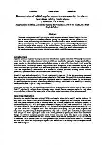
Figure 1. Four vector beams with azimuthal variant state of polarization (SOP) generated with equation (8) are shown in four row panels, corresponding to (a-d). In each panel, different sketches of SOP trace on Poincaré sphere marked by red line, SOP distribution in space and snap picture of SOP are demonstrated in order. Associated parameters in equation (8) for field generation are (a) lL , lR 1,3 / 30 , (b) lL , lR 1,3 / 120 , (c) lL , lR 2,1 / 60 , and (d) lL , lR 2,1 / 135 , respectively.
the OAM charge can be obtained as l lR L
lL lR R L l 2
2
TPC
R L gO .
(11)
In the right side of equation (11), the first term corresponds to topological Pancharatnam’s charge ( lTPC ), which is referenced to right or right circularly polarized R L field and just equals to lR(L) in this case. In the second term, gO lL lR R L 4
is the OAM-dependent geometric phase induced by space-variant SOP, which corresponds to the reported result in Ref. [10]. Equation (11) explicitly reveals that the OAM charge is not only related with topological Pancharatnam’s charge lTPC but also R L the geometric phase gO of OAM-dependent (is proportional to lL lR 2 ). For more
clarity, some simulations have been carried on four fields generated with equation (8) and the results are shown in Fig. 1. Figures 1(a-d) are the calculated results while the parameters are set as
lL , lR 1,3 with 30 and
120 and
lL , lR 2,1 with 60 and
135 .
For each row panel, there are three parts in order: SOP trace on Poincaré sphere marked by red line, SOP distribution in space, and a SOP snap in space. In Fig. 2, calculated results of OAM charges are shown as the dots, which are calculated by equation (11) for the four cases shown in Figs. 1(a-d). For comparison, the OAM charges are also calculated by mode expansion method according to equation (8) and shown as solid lines in Fig.2. For the cases shown in Figs. 1(a) and (b), the left circularly polarized fields (North Pole on Poincaré sphere) is selected as the reference
5
Figure 2. The calculated OAM charge for the vector beams generated with equation (8) of lL , lR 1,3 and 2,1 at different zenith angle in spherical coordinate (Poincaré sphere). Dots are OAM charges are calculated with our formula, which are corresponding to cases shown in Figs. 1(a-d), respectively. Solid lines are calculated by mode expansion method according to equation (8).
field and enclosed surface areas are also shown with yellow zone. While for Fig. 1(c) and (d), right circularly polarized field (South Pole on Poincaré sphere) is selected as the reference. In Fig.2, all the calculated results with our formula are in good agreement with those calculated by mode expansion method. From the results shown in Figs. 1 and 2, a clear relation of OAM charge versus Pancharatnam’s phase and geometric phase is presented. Furthermore, with our formula, a geometrical description of OAM can be obtained by utilizing a basic Poincaré sphere. (b) Vectorial vortex beam generated by phased array antenna Recently, more and more attentions have been focused on the generation of OAM beams with phased array antenna (PAA) in RF, microwave, and lightwave region [27-29]. To model such process, some simulations are also carried on an annular PAA with antenna unit of linearly polarized Gauss beam as schematically shown in Fig. 3(a). In the simulations, the optical communication wavelength of 1550 nm is adopted. For each Gauss beam, the waist size is 8 μm and polarization direction is azimuthal-dependent. The unit number is 16 and radius ( R ) of annular PAA, which is defined by the distance between the PAA center and each unit center as marked in Fig. 3(a), can be adjusted. These parameters ensure that the generated beam satisfies the paraxial approximation, thus Barnett’s method [3] can be utilized as a reference with the results calculated by equation (7). As demonstrated in Ref. [28], the AM charges of the generated beam can be tuned by varying the phase difference between adjacent units. In our simulation, the adjacent phase differences are uniform and the whole feeding phase of a circle ( F ) is used to descript the setting phase on each antenna. With such a structure, various vortex beams can be generated, such as radially or azimuthally polarized vector beams, L-line vortex beams [30], and so on.
6
Figure 3. (a) Schematic of the considered phased array antenna (PAA), which consists of 16 units. Each unit emits linearly polarized Gauss beam and the polarization direction and initial phase can be set. With PAA, varied vectorial vortex beams can be generated, (b) state of polarization (SOP) makes two revolutions at latitude on Poincaré sphere (radially polarized vectorial beam), (c) SOP makes one revolution (L-line vortex), and (d) SOP makes half revolution.
Figure 3(b) shows a radially polarized vectorial beam, where SOP makes two revolutions at latitude on Poincaré sphere for a circle in the space. Corresponding AM charges are calculated by both Barnett’s method and our formula, which are shown as lines and dots in Fig. 4(a), respectively. Two cases with different PAA radius of 10 and 30 μm are also considered under the varied feeding phase, both methods give consistent OAM charge. Furthermore, Fig. 3(c) and (d) display another two types of vortex beam, where SOP makes one and half revolution at latitude on Poincaré sphere for a circle in the space, respectively. For a fixed PAA radius of 20 μm, the OAM charges at different feeding phase are also calculated and presented in Fig. 4(b), and again, they are also in a very good agreement. These results indicate that the calculations for OAM charge with equation (7) can be applied on not only general vector beams but also complex vortex beams with the paraxial approximation. Moreover, it should be noticed that for most general vector beam shown in Fig. 3(b), the feeding phase F are transferred to both OAM and SAM (see Fig. 4(a)), which is quite different to the scalar vortex beam. For a scalar vortex beam, the feeding phase F would be fully transferred to OAM. Even when F is 2N ( N is any integer
number), the total angular momentum (TAM) charge equals to N , which is not the value of OAM charge (recently, a similar report was presented in Ref. [31]). The reason is that some AM is transferred to SAM in the central zone of vortex as shown with
7
Figure 4. Calculated angular momentum (AM) charges of (a) the vortex beam shown in Fig. 3(b) at different feeding phase of two different PAA radius of 10 and 30 μm, and (b) the vortex beam shown in Fig. 3(c) and 3(d) at different feeding phase of fixed PAA radius of 20 μm. In the figures, lines are calculated by Barnett’s method and symbols are calculated by our formula for OAM and Stoke parameter of s3 for SAM. Right-side insets also show the corresponding SOP distribution at feed phase equals 2 .
yellow color in right-side inset of Fig. 4(a) and meanwhile the reduction of solid angle of surface area on Poincaré sphere would suppress the transformation of OAM from feeding phase. Fortunately, through a carefully designed PAA, the proportion of OAM charge can be varied by reducing power proportion of field around vortex center. Likewise, because of partial OAM induced by geometric phase, the detection of OAM charge will be different with that for scalar vortex by only detecting phase angle of wavefront. Thus, to detect OAM charge of vectorial vortices, new method is required. We predict that such detection can be achieved by traditional measurement of Stokes parameters according to equation (7).
8
4
Conclusion In conclusion, it is found that, for vectorial vortices, the OAM charge is not only
related with the topological Pancharatnam’s charge but also the geometric phase induced by space-variant state of polarization. Based on such a connection, OAM also can be fully represented by the basic Poincaré sphere. And we predict that the detection of OAM charge can be achieved by testing Stokes parameters, which is a standard test of polarization measurement for antennas. Moreover, because of the explicit relation with geometric phase, we believe that this work would give some new insights for studies on vectorial vortices, spin-orbit interaction, photonic topological insulators, and so on.
Acknowledgements This work was supported by the National Basic Research Program of China (No. 2011CBA00608, 2011CBA00303, 2011CB301803, and 2010CB327405), the National Natural Science Foundation of China (Grant No. 61036010, 61036011 and 61321004) and by the Opened Fund of the State Key Laboratory on Integrated Optoelectronics, China. No. IOSKL2013KF09. The authors would like to thank Yu Wang and Peng Zhao for their valuable discussions and helpful comments.
References [1]. M. Padgett, J. Courtial and L. Allen, Physics Today 57, 35 (2004). [2]. S. Franke-Arnold, L. Allen and M. Padgett, Laser & Photonics Review 2, 299 (2008). [3]. S. M. Barnett, Journal of Optics B: Quantum and Semiclassical Optics 4, S7 (2002). [4]. A. M. Yao and M. J. Padgett, Advances in Optics and Photonics 3, 161 (2011). [5]. L. Allen, M. Beijersbergen, R. Spreeuw and J. Woerdman, Physical Review A 45, 8185 (1992). [6]. X.-L. Wang, J. Chen, Y. Li, J. Ding, C.-S. Guo and H.-T. Wang, Physical Review Letters 105, 253602 (2010). [7]. Z. Bomzon, G. Biener, V. Kleiner and E. Hasman, Optics letters 27, 1141 (2002). [8]. Z. Bomzon, G. Biener, V. Kleiner and E. Hasman, Optics letters 27, 285 (2002). [9]. A. Niv, G. Biener, V. Kleiner and E. Hasman, Optics express 14, 4208 (2006). [10]. G. Milione, S. Evans, D. A. Nolan and R. R. Alfano, Physical Review Letters
9
108, 190401 (2012). [11]. G. Milione, H. I. Sztul, D. A. Nolan and R. R. Alfano, Physical Review Letters 107, 053601 (2011). [12]. M. J. Padgett and J. Courtial, Optics letters 24, 430 (1999). [13]. F. Tamburini, E. Mari, A. Sponselli, B. Thidé, A. Bianchini and F. Romanato, New Journal of Physics 14, 033001 (2012). [14]. J. Wang, J.-Y. Yang, I. M. Fazal, N. Ahmed, Y. Yan, H. Huang, Y. Ren, Y. Yue, S. Dolinar, M. Tur and A. E. Willner, Nature Photonics 6, 488 (2012). [15]. A. Nicolas, L. Veissier, L. Giner, E. Giacobino, D. Maxein and J. Laurat, Nature Photonics 8, 234 (2014). [16]. E. Galvez, P. Crawford, H. Sztul, M. Pysher, P. Haglin and R. Williams, Physical Review Letters 90, 203901 (2003). [17]. K. Bliokh, Physical Review Letters 97, 043901 (2006). [18]. A. Aiello, N. Lindlein, C. Marquardt and G. Leuchs, Physical Review Letters 103, 100401 (2009). [19]. K. Bliokh, Y. Gorodetski, V. Kleiner and E. Hasman, Physical Review Letters 101, 030404 (2008). [20]. E. Karimi, S. Slussarenko, B. Piccirillo, L. Marrucci and E. Santamato, Physical Review A 81, 053813 (2010). [21]. K. Y. Bliokh, A. Niv, V. Kleiner and E. Hasman, Nature Photonics 2, 748 (2008). [22]. J. P. Torres and L. Torner, Twisted Photons: Applications of Light with Orbital Angular Momentum. (John Wiley & Sons, 2011). [23]. M. Born and E. Wolf, Principles of optics: electromagnetic theory of propagation, interference and diffraction of light. (CUP Archive, 1999). [24]. L. Allen and M. J. Padgett, Optics Communications 184, 67 (2000). [25]. M. V. Berry, Journal of Modern Optics 34, 1401 (1987). [26]. C. Maurer, A. Jesacher, S. Fürhapter, S. Bernet and M. Ritsch-Marte, New Journal of Physics 9, 78 (2007). [27]. S. M. Mohammadi, L. K. S. Daldorff, J. E. S. Bergman, R. L. Karlsson, B. Thidé, K. Forozesh, T. D. Carozzi and B. Isham, Antennas and Propagation, IEEE Transactions on 58, 565 (2010). [28]. D. Zhang, X. Feng and Y. Huang, Optics express 20, 26986 (2012). [29]. X. Cai, J. Wang, M. Strain, B. Johnson-Morris, J. Zhu, M. Sorel, J. O'Brien, M. Thompson and S. Yu, Science 338, 363 (2012). [30]. J. F. Nye, Proceedings of the Royal Society A: Mathematical, Physical and Engineering Sciences 389, 279 (1983). [31]. J. Zhu, Y. Chen, Y. Zhang, X. Cai and S. Yu, Optics Letters 39, 4435 (2014).
10
Supplementary Material A. Relation of orbital angular momentum, Pancharatnam’s phase, and geometric phase For a vectorial vortex beam of angular frequency propagate along z direction, in the paraxial approximation, the electric and magnetic fields can be written as [22] i ikz E x, y i xˆ yˆ zˆ e , k x y
(S1a)
i ikz B x, y ik xˆ ayˆ zˆ e , k x y
(S1b)
where and represent the complex amplitude of x and y component of electric field, and further they can be written as Ax ( x, y ) e i x ( x , y ) ,
(S2a)
Ay ( x, y ) e i y ( x , y ) ,
(S2b)
where Ax y and x y are real numbers and represent amplitude and phase, respectively. Further, Stokes parameters are defined by [23] s0 A x2 A y2 s1 A x2 A y2
(S3)
s2 2 A x A y cos s s3 2 A x A y sin s
where A x y Ax y I E are normalized electric field components with electric intensity of I E Ax2 Ay2 , and s y x is the phase difference between x and y electric field components. Then using s1 , s2 , and s3 as the sphere’s Cartesian
coordinates, Poincaré sphere is constructed and its spherical angles resolved by [23]
2 S , 2 S is
tan(2 S ) s2 s1 ,
(S4a)
sin(2 S ) s3 s0 .
(S4b)
According to the definition of linear momentum density of p 0 E B , it can be
written and divided into 0 p i 2 zˆ , 2
2
pz k 0
11
2
k I s . 0 E 0
(S5a) (S5b)
Meanwhile, the energy density of such a beam is
2
w cpz 0 2
2
I s . 0
2
E 0
(S6)
Then, using line momentum density, the cross product with r (radius vector) gives
the angular momentum density, and z component of angular momentum density is jz r p z rp i
0 2
2r . r
(S7)
Further, jz can be divided into spin and orbital parts as jzspin i 0 r
I E s3 0 r , r r
0 2 x 2 y 0 I E A x2 Ay .
(S8a)
jzorbit i
(S8b)
With the ratio of angular momentum to energy examined by Allen [24], the average SAM charge and OAM charge of a vortex beam can be calculated as spin z
j rdrd I s wrdrd I l
jzorbit rdrd
wrdrd
I
E
s rdrd
E 3
s rdrd
,
(S9a)
E 0
2 x 2 y Ay Ax rdrd . I E s0 rdrd
(S9b)
Then, introducing Pancharatnam’s phase, which is defined by [25] P arg A B .
(S10)
Here, using right or left circularly polarized fields as reference field, for any field E xˆ yˆ , its Pancharatnam’s Phase is written as
PR(L) arg R(L) E .
(S11)
Then we can get tan PR(L)
A y cos y A x sin x . A y sin y A x cos x
12
(S12)
Further, we deduced PR 1 tan PR 1 tan 2 PR
cos s s0 s3
A y A x s3 x y 1 2 x 2 y Ay Ay Ax Ax 2 s s s 0 3 0 s3
(S13a) PL 1 tan PL 2 1 tan PL cos s A y A x s3 x y 1 2 x 2 y Ay Ay Ax Ax s0 s3 2 s0 s3 s0 s3
(S13b) On the other hand, using equations (S4a) and (S3), we get S 1 tan 2 S 2 2 1 tan 2 S
With
relation
s0 cos s s02 s32
A y A x y x s1 s3 Ay Ax . 2 2 2 s0 s3
x y y x 2 x 2 y s0 Ay s1 2 Ax
of
(S14)
and
equations (S13a), (S13b), and (S14), we get s0
PR S 2 x 2 y (s0 s3 ) Ax Ay ,
(S15a)
PL S 2 x 2 y (s0 s3 ) Ax Ay .
(S15b)
s0
Through further derivation with equations (S15a) and (S15b), we can get, PR L x 2 y S A x2 Ay s0 (s0 s3 ) .
(S16)
Then, substituting equation (S16) into equation (S9b), we can solve the OAM charge. In equation (S16), the first term is the gradient of spiral spatial phase known as topological Pancharatnam’s charge, and the second term is related to geometric phase induced by space-variant SOP. B. For the case of vector beams generated by two scalar vortex beams
13
General vector beam can be generated by mode expansion as [26] E
1 cos xˆ iyˆ e ilL sin xˆ iyˆ e ilR . 2 2 2 2
1
(S17)
Thus, with equation (S11), we get PR L
(S18)
lR(L) .
And, we deduced s1 sin cos lL lR 0 ,
(S19)
s2 sin sin lL lR 0 .
So, with equations (S4a) and (S3), we get S lL lR 0 2.
(S20)
S lL lR 2.
(S21)
Then,
Substituting equations (S18) and (S21) into equations (S9b) and (S16), OAM charge can written as l lR
lL lR
l lL
2
R 1 sin 2 S lTPC
lL lR 2
lL lR R
L 1 sin 2 S lTPC
2
2
lL lR L 2
2
R lTPC
R gO ,
L lTPC
L gO .
(S22a) (S22b)
R(L) where lTPC lR(L) is topological Pancharatnam’s charge that is referenced to right (left) circularly polarized field, R L is the solid angle of surface area on Poincaré sphere
R L enclosed by trace of SOP and south (north) pole, and the gO is the OAM-dependent
geometric phase induced by space-variant SOP.
14