Available online at www.sciencedirect.com
ScienceDirect Procedia Computer Science 55 (2015) 18 – 27
Information Technology and Quantitative Management (ITQM 2015)
Identifying problem solving strategies for learning styles in engineering students subjected to intelligence test and EEG monitoring Felisa M. Córdovaa,*, Hernán Díaz M.a, Fernando Cifuentesa, Lucio Cañeteb, Fredi Palominosc a
Department of Industrial Engineering, Faculty of Engineering b Faculty of General Technologies c Department of Mathematic and Computer Science, Faculty of Science University of Santiago de Chile. Av. Ecuador 3469, Santiago 9170124, Chile.
Abstract The cognitive approach of learning agrees in that behavior of the individual correlates with certain complex and dynamic mental processing operations modulated by certain internal mechanisms learned or improved during life. Applied to university learning, the demand towards students no longer focuses only in the results of the process but, ideally, in the development of individual styles based on cognitive preferences and learning strategies. Several tests such as Kolb and VAK or Hermann dominances allow distinguishing some learning styles such as: Divergent, Assimilator, Convergent and Accommodator; Visual; Kinesthetic; and Auditory. Meanwhile, by using electrophysiological tools like an electroencephalographic (EEG) recording it is now possible to measure individual differences in the varying electrical activity present in the cerebral cortex while a student face a cognitive problem or performs a test of intelligence. In this study, we tested 20 students from their early years of engineering to be classified in three systems of learning styles. The students were then subjected to a test of intelligence (Raven test, abbreviated version of 15 questions) with increasing levels of complexity. The time length to solve the test taken for students previously classified in four main styles yielded by the Kolb test, were analyzed. Then we grouped them by correspondences with the visual, auditory and kinesthetic predominance yielded by the VAK test. The response time was measured and the absolute frequency of response time for each question was calculated. During the Raven test execution an electroencephalogram with Emotiv Epoc Brain-Computer Interface of 14 channels was recorded. After subtracting baseline and eliminating common artifacts with the help of EEGLAB toolbox under Matlab, we obtained clean signals for theta, alpha, beta and gamma bands. Using the set of learning styles classificatory tools and the electrophysiological analysis we started to look for variability and consistencies that support or rise new questions about adequate usefulness of common used psycho-cognitive and behavioral learning styles tests. In our sample we found relatively low discriminative resolution from all learning styles test applied, but a promising research field to study electrical brain activity phenomenology associated with learning and solving problem strategies of the brain. © by Elsevier B.V. This is an open access article under the CC BY-NC-ND license © 2015 2015Published The Authors. Published by Elsevier B.V. (http://creativecommons.org/licenses/by-nc-nd/4.0/). Selection and/or peer-review under responsibility of the organizers of ITQM 2015 Peer-review under responsibility of the Organizing Committee of ITQM 2015 Keywords: Learning style; Intelligence test; problem solving strategies, EEG.
* Felisa Córdova. Tel.: +56-2-23260268; fax: +56-2-23260268. E-mail address:
[email protected]
1877-0509 © 2015 Published by Elsevier B.V. This is an open access article under the CC BY-NC-ND license (http://creativecommons.org/licenses/by-nc-nd/4.0/). Peer-review under responsibility of the Organizing Committee of ITQM 2015 doi:10.1016/j.procs.2015.07.003
Felisa M. Córdova et al. / Procedia Computer Science 55 (2015) 18 – 27
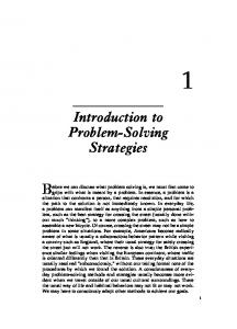
1. Introduction The performance of a human being in solving a problem that involves cognitive processing is determined by a neuro-cognitive individuality which is being built during the progressive (or regressive) brain development. Several of these individualities are usually present in a cryptic status and, in teaching-learning environments, they are hardly noticeable for teachers in the classroom as to using this information to plan or improve educational process. To find some of these hidden variables we may need to turn more explicit the neurocognitive mechanism underlying problem solving processing occurring in the brain. We can do this through the study of a set of biometric variables whose correlations and phenomenology can enlighten our understanding of the individual functional processes taking place in the brain. A better understanding and monitoring of such processes would help to select and support improved variants or new teaching strategies inspired in the acquired knowledge coming from this field research. It is expected that this improvement in knowing underlying cognitive problem solving processes that may help to explain cognitive individualities will impact positively on the improvement, efficiency and effectiveness of teaching and learning processes. To classify inter-individual differences and to group them into categories of learning strategies, there has been developed several theories, for example, Gardner´s multiple intelligences, which in principle considers eight different ways to deal with knowledge acquisition [1]. According to this idea eight different types of skills or intelligences can be distinguished. These define the way(s) each individual faces, understands, deals, or tries to solve a given problem or a particular cognitive or behavioral challenge. The eight kinds of intelligences proposed are: linguistic; logical-mathematical; spatial; musical; corporal-kinesthetic; intra-personal; interpersonal; and naturalistic. Since this initial classification, other authors also have defined and grouped human diversity in the context of knowledge acquisition and processing preferences in learning. Such is the case of the classification coming from neurolinguistic programming (NLP) that classifies individuals into three categories according to their preferred way to capture and process information from the environment [2]. Here, people can be classified as visual, auditory or kinesthetic, depending on which sense dominates on the initial data acquisition and processing of information. In another proposal, Kolb developed a scheme of four orthogonal axes whose quadrants define a combination of preferences or styles that determine a specific way to deal with problem solving [3]. In this scheme, a person can have one, or a combination, of the following styles: accommodator; convergent; assimilator; and divergent, according to his/her preference for: concrete experience; active experimentation; abstract conceptualization; and reflective observation (Fig 1). Another system proposed by Alonso [4] classifies people in: reflective; pragmatic; active; and theoretical. All categories intersect each other to some extent with the models mentioned above.
Fig. 1. Kolb’s classification of learning styles
Other authors incorporate a biological-evolutionary component concerning development of cognitive and learning processing, integrating the results of several contemporary neurophysiologists who argue that the cerebral cortex exert voluntary control over the emotional aspects [5-6-7]. In this sense, in the model of "brain dominances", Herrmann proposes that the brain works in four predominant operating modules that meet certain broad localization in the brain [8]. Thus, brain is divided into four modules: two frontal regions (left and right)
19
20
Felisa M. Córdova et al. / Procedia Computer Science 55 (2015) 18 – 27
and two inferior or lateral regions (left and right) [9]. Frontal regions correspond to the part of the cortex that specializes in modulating and control of emotions where rationality, planning and foresight are included; while lower regions are related to less modulated emotions and interpersonal skills. The development of techniques to measure brain function has been mainly related to the study and diagnosis of developmental disorders and/or learning dysfunctions [10-11-12]. In our context it would be useful to create a broader classification tool that includes non-diagnosed or medically treated people, to establish first a local baseline framework against with to compare. In a teaching context, to count with such a characterization of cognitive variability and brain processing preferences must encourage education researchers to take advantage of it including as well the value and importance of emotions, it plays a role either helping or hindering the learning process and development [13-14]. In his classical approach, Piaget identified stages of cognitive development, depending on the age, for handling scientific knowledge, integrating these findings into the practice of learning and teaching in the school [15]. The progressive ease of implementing a model which can allows us to test, analyze and diagnose brain functional states by using simple brain-computer interfaces facilitates the nowadays access to the study of the brain processes involved in different aspects of learning. Current technological advances has allowed researchers to mine into the cryptic aspects of this process revealing, identifying and using neuro-cognitive and behavioral correlates for brain control of a machine [16]. All the information that has coming to light in this rather new research field can be used to improve our knowledge of teaching-learning process by using that evidence to understand, implement and test teaching strategies built on a neuroscience applied to practical (and not only theoretical) solutions for education. Braincomputer-machine interfaces expand the capacity of engineer and neurobiology to follow, record, and statistically explore the signal of brain activity, during its ongoing functional coupling with the environment in daily-life circumstances. To date there are rather few applications of recent finding oriented to education to unveil more deeply the mid- and long-term intimacy of neuro-cognitive processes of students in the teachinglearning process [17]. By integrating neurophysiology and automatic has been possible to achieve powerful applications which help to reveal part of this neuro-cognitive intimacy [18-19-20]. By using headbands to record brain activity, it is possible to detect patterns of electroencephalographic response in front of the challenge of learning. Concurrently, there has been a major breakthrough in the field of data analysis and pattern recognition, attempting to identify correlations between neurophysiology and behavior in complex environments [14]. Applied to teaching and learning processes it can help to improve the knowledge about inter-individual differences and preferences in information processing strategies by students, to improve and test new variants in teaching and learning strategies. In this paper we explore some of the individualities involved in the process of solving a cognitive problem, analyzing the response time of the students solving 15 questions of a visual intelligence test (Raven Test, abbreviated version) while simultaneous EEG recording. 2. Method 2.1. Classification of learning styles in the experimental group In order to diagnose the main cognitive styles involved in learning processing of first-year engineering students, a group of 20 undergraduates were randomly chosen. Each student was also asked to answer a set of psycho-behavioral tests (Kolb, VAK, and Herrmann´s Brain Dominances). The results of this analysis are presented in a matrix composed of a set of variables associated with learning styles: visual (V), auditory (A), kinesthetic (K), convergent, divergent assimilator, accommodator (K1, K2, K3, K4) and the 4 types of Herrmann´s brain dominances (A, B, C, D). 2.2. Raven’s (abbreviated version) progressive matrices test The Raven’s Progressive Matrices test is a non-verbal test which can be applied in individual or collective situation. It consists of a number of problems in which the students selects missing pieces of a chart in order to complete a drawing. Operationally, the task consists in compare forms and reason by analogy. The test used corresponds to a shortened version (15 questions) of the original Raven´s test that is presented in the computer
21
Felisa M. Córdova et al. / Procedia Computer Science 55 (2015) 18 – 27
screen. The responses are recorded in real time and then are reviewed to determine in which time frame each matrix was answered. 2.3. EEG monitoring To investigate the brain activity phenomenology during the test solving process and to search for potential correlates between different classificatory variables and brain activity, we simultaneously recorded the electroencephalographic signal (EEG) making possible to study some of the electrophysiological characteristics of the brain signal during the whole response time period and during processing specific questions. The EEG recording consisted in a basal, resting state, recording with open and closed eyes, minutes before the initiation of the test execution. A further recording was captured during the whole resolution of the test. We used the non-invasive brain computer device Emotiv EPOC® [21] to record 14 channels from head locations according to the standard 10/20 system. After subtracting the baseline and eliminating common signal artifacts with the help of EEGLAB and ADJUST [22] toolbox under Matlab, we obtained clean signals for the theta, alpha, beta and gamma bands. These signals reflect the dynamics of each student's brain operation in conditions of resting quiet awake and during the execution of the abbreviated version of Raven’s test. 2.4. Analysis of response time to the Raven test according to combination of learning styles The results of the measurements were tabulated and entered into a database for further analysis using Matlab. Response time in Raven’s test used by representative students of cognitive styles: convergent, divergent assimilator and accommodator were analyzed, selecting the cases of visual preference rendered by VAK test. 3. Results Table 1 shows the classification results rendered by the three psycho-behavioral tests applied to 20 engineering students. Table 1. Results of Kolb, VAK and brain dominance tests for the 20 engineering students
Student 1 2 3 4 5 6 7 8 9 10 11 12 13 14 15 16 17 18 19 20
V 1 4 5 5 2 3 1 2 2 1 3 3 4 1 3 2 4 2 2 2
VAK K 3 2 1 0 2 2 3 4 2 4 1 1 1 1 2 3 1 3 2 3
A 3 1 1 2 3 2 3 1 3 2 3 3 2 5 2 2 2 2 3 2
K1 27 18 16 24 23 19 43 22 32 26 25 33 18 38 15 29 21 20 12 32
K2 30 39 42 27 41 29 14 30 25 26 32 34 35 27 29 17 21 33 46 32
KOLB K3 35 39 38 38 27 37 25 34 20 37 43 28 33 39 41 41 47 31 31 24
K4 28 24 24 31 29 35 38 34 43 28 20 25 36 16 35 33 31 36 31 32
A 39 39 40 37 35 34 32 42 25 33 45 30 45 41 44 45 40 41 39 31
Brain B 48 36 34 35 37 32 35 44 35 34 33 32 47 25 43 43 40 39 44 31
Dom C 33 33 29 29 42 31 34 39 43 31 25 30 43 46 29 35 42 37 42 33
D 36 31 36 32 31 31 33 36 35 34 39 24 42 32 30 41 49 40 20 32
As the Raven test is predominantly visual, students are grouped by VAK Learning Style in three clusters using k-means with k = 3. The vector of the centroid for each VAK style is shown in Table 2. Table 2. Vector of the centroid for VAK learning style in 20 engineering students
22
Felisa M. Córdova et al. / Procedia Computer Science 55 (2015) 18 – 27
Vector Kinesthesis (1) Auditory (2) Visual (3)
V 1.5714 1.7500 3.7778
Centroid K 3.2857 1.7500 1.2222
A 2.1429 3.5000 2.0000
Once separated in VAK categories: visual (subjects 1,7,8,10,16,18,20); kinesthetic (5,9,14,19); and auditory (2,3,4,6,11,12,13,15,17), we considered the cluster of students with visual tendency first and this data was crossed with the Kolb Learning Style classification. Each point on the Kolb’s map of learning styles represents a vector in the plane. The Euclidean length of this vector is calculated and then divided by the maximum score. The result is multiplied by 100 and the "percentage of ownership within each quadrant (or Kolb type)" is obtained. Fig 2 shows the coordinates within the quadrant corresponding to the Kolb’s Learning Style for 20 students. Results from the comparison of "Visual students" with the Kolb classification are shown in Table 3.
Fig. 2. Map of Learning Styles for 20 students according Kolb’s classification Table 3. Visual Students (according to VAK) associated to Kolb Learning Style
Student 6 15 13 17 4 12 11 2 3
VAK (Visual Cluster data only) V K A 3 2 2 3 2 2 4 1 2 4 1 2 5 0 2 3 1 3 3 1 3 4 2 1 5 1 1
KOLB learning Style Quadrant Kolb Classification Kolb Percentage 1 Divergent 39.5 1 Divergent 55.6 1 Divergent 31.3 1 Divergent 58.0 1 Divergent 30.3 3 Convergent 21.4 4 Accommodator 45.1 4 Accommodator 53.8 4 Accommodator 59.2
For students with Kinesthesis dominance, when collated according Kolb classification, Table 4 is obtained.
Table 4. Kinesthetic Students (according to VAK test) associated with Kolb Learning Styles.
23
Felisa M. Córdova et al. / Procedia Computer Science 55 (2015) 18 – 27
Student 10 8 16 18 7 1 20
VAK (Kinesthetic Cluster data) V K A 1 4 2 2 4 1 2 3 2 2 3 2 1 3 3 1 3 3 2 3 2
KOLB learning Style Quadrant Kolb Classification Kolb Percentage 1 Divergent 23.29 1 Divergent 26.35 1 Divergent 41.67 1 Divergent 23.75 2 Assimilator 62.50 3 Accommodator 17.18 4 Assimilator-Converger 16.67
For students with auditory predominance, when collated according Kolb classification, Table 5 is obtained. Table 5. Auditory students (according to VAK test) associated with Kolb Learning Styles. VAK (Auditory Cluster data only) Student 14 5 19 9
V 1 2 2 2
K 1 2 2 2
A 5 3 3 3
KOLB Learning Style Quadrant 4 4 4 2
KOLB Classification Accommodator Accommodator Accommodator Assimilator
KOLB Percentage 23.01 26.35 50.43 45.07
Under the assumption that the response times in the Raven test for each student is a characteristic of the student and with the aim to make response times comparable, response time for each matrix was normalized as follows: the time spent on the solution of each matrix is divided by the total time spent in answering the Raven test completely. The results are shown in Table 6. The normalized times are dimensionless since a partial time is divided by a total time. Then, this table shows the absolute frequency of the response time for each matrix in the Raven test. Table 6. Standardized times of all students (20 students) for each matrix of the Raven test Student 1 2 3 4 5 6 7 8 9 10 11 12 13 14 15 16 17 18 19 20
M1 0.0098 0.0247 0.0198 0.0188 0.0198 0.0197 0.0392 0.0378 0.0172 0.0095 0.0168 0.0649 0.0682 0.0338 0.0280 0.0379 0.0247 0.0837 0.0231 0.0582
M2 0.0075 0.0132 0.0181 0.0193 0.0135 0.0175 0.0268 0.0209 0.0363 0.0105 0.0145 0.0233 0.0226 0.0168 0.0220 0.0221 0.0373 0.0236 0.0158 0.0738
M3 0.0359 0.0178 0.0266 0.0171 0.0157 0.0319 0.0564 0.0815 0.0231 0.0258 0.0321 0.0213 0.0126 0.0228 0.0647 0.0752 0.0319 0.0309 0.0212 0.0670
M4 0.0126 0.0134 0.0215 0.0205 0.0305 0.0233 0.0246 0.0256 0.0316 0.0150 0.0156 0.0207 0.0195 0.0168 0.0451 0.0321 0.0252 0.0229 0.0162 0.0472
M5 0.0237 0.0165 0.0204 0.0267 0.0264 0.0285 0.0397 0.0457 0.0243 0.0171 0.0336 0.0351 0.0290 0.0140 0.0480 0.0292 0.0445 0.0254 0.0319 0.0515
M6 0.0620 0.0480 0.0224 0.0398 0.0387 0.0750 0.0872 0.0586 0.0612 0.0481 0.0360 0.0412 0.0758 0.1169 0.0707 0.1004 0.0752 0.0371 0.0758 0.0695
M7 0.0177 0.0233 0.0376 0.0689 0.0428 0.1377 0.0603 0.0480 0.0678 0.0405 0.0172 0.0331 0.0430 0.0215 0.0237 0.0437 0.0697 0.0262 0.0366 0.0650
M8 0.0104 0.0217 0.0295 0.0461 0.0350 0.0378 0.0519 0.0485 0.0499 0.0256 0.0254 0.0351 0.0373 0.0140 0.0327 0.0275 0.0385 0.0283 0.0232 0.0580
M9 0.0472 0.0855 0.0967 0.0637 0.0791 0.0610 0.0838 0.0404 0.1069 0.1067 0.0931 0.0535 0.0879 0.0490 0.0517 0.1084 0.0998 0.0558 0.0878 0.0517
M10 0.0376 0.0252 0.0563 0.0502 0.0383 0.0540 0.0508 0.0457 0.0781 0.0344 0.0481 0.0538 0.0444 0.0251 0.0490 0.0407 0.0583 0.0484 0.0431 0.0855
M11 0.0702 0.0819 0.0862 0.1461 0.0396 0.0831 0.0631 0.0531 0.0665 0.1403 0.0466 0.0676 0.0961 0.0793 0.0667 0.0658 0.0835 0.0628 0.1391 0.0711
M12 0.1467 0.1786 0.1768 0.1997 0.1190 0.1099 0.1330 0.0932 0.1624 0.2159 0.1392 0.1331 0.1119 0.2445 0.1624 0.1602 0.0824 0.1028 0.1092 0.0828
M13 0.1306 0.0430 0.0686 0.1161 0.0881 0.0593 0.0670 0.0545 0.0868 0.0397 0.0532 0.1632 0.0690 0.0681 0.1124 0.0668 0.0602 0.0909 0.1438 0.0722
M14 0.1718 0.1738 0.0757 0.0460 0.2611 0.1336 0.0772 0.1589 0.0415 0.1054 0.2663 0.1711 0.0656 0.2061 0.0864 0.1195 0.1425 0.1230 0.1267 0.0802
M15 0.2164 0.2334 0.2439 0.1212 0.1524 0.1279 0.1391 0.1876 0.1462 0.1655 0.1623 0.0830 0.2171 0.0713 0.1367 0.0703 0.1263 0.2382 0.1064 0.0664
By selecting the normalized response times of the Raven test answer for Visual students according to VAK classification and sorted by Kolb learning Styles, presented in Table 3, Table 7 is generated.
24
Felisa M. Córdova et al. / Procedia Computer Science 55 (2015) 18 – 27
Table 7. Normalized response time for Visual students, including Kolb classification Student 6 15 13 17 4 12 11 2 3
M1 0.0197 0.0280 0.0682 0.0247 0.0188 0.0649 0.0168 0.0247 0.0198
M2 0.0175 0.0220 0.0226 0.0373 0.0193 0.0233 0.0145 0.0132 0.0181
M3 0.0319 0.0647 0.0126 0.0319 0.0171 0.0213 0.0321 0.0178 0.0266
M4 0.0233 0.0451 0.0195 0.0252 0.0205 0.0207 0.0156 0.0134 0.0215
M5 0.0285 0.0480 0.0290 0.0445 0.0267 0.0351 0.0336 0.0165 0.0204
M6 0.0750 0.707 0.0758 0.0752 0.0398 0.0412 0.0360 0.0480 0.0224
M7 0.1377 0.0237 0.0430 0.0697 0.0689 0.0331 0.0172 0.0233 0.0376
M8 0.0378 0.0327 0.0373 0.0385 0.0461 0.0351 0.0254 0.0217 0.0295
M9 0.0610 0.0517 0.0879 0.0998 0.0637 0.0535 0.0931 0.0855 0.0967
M10 0.0540 0.0490 0.0444 0.0583 0.0502 0.0538 0.0481 0.0252 0.0563
M11 0.0831 0.0667 0.0961 0.0835 0.1461 0.0676 0.0466 0.0819 0.0862
M12 0.1099 0.1624 0.1119 0.0824 0.1997 0.1331 0.1392 0.1786 0.1768
M13 0.0593 0.1124 0.0690 0.0602 0.1161 0.1632 0.0532 0.0430 0.0686
M14 0.1336 0.0864 0.0656 0.1425 0.0460 0.1711 0.2663 0.1738 0.0757
M15 0.1279 0.1367 0.2171 0.1263 0.1212 0.0830 0.1623 0.2334 0.2439
The time spent to solve each Raven´s matrix represents a proxy measure for the load of cognitive process involved in the problem solving task, or the relative difficulty that each matrix poses on each subject. Total time spent is not a variable taken into account to estimate a range value for intelligence quotient (IQ) and besides individual differences in the time spent solving each matrix, a general trend to higher cognitive load or matrix difficulty is evident. Fig 3 shows three examples of characteristic non-normalized time course development during solving 15 Raven´s matrices. Y axis represents time duration in seconds, while X axis order the correlative matrices solved, M1 to M15.
Fig. 3. Three examples of representative time duration development for solving 15 Raven´s test matrices
IQ ranges yielded by the abbreviated version for Raven’s test does not group students in a clear classification according Learning Styles but a slightly trend can be seen in the 95-120 IQ range where 7 out of 10 subjects were categorized as visual according VAK test. Other IQ ranges have few subjects as to make a similar tentative conclusion connecting Raven test results and learning preferences. Table 8 shows IQ range estimation results. Considering that Raven’s Test Matrices is a test of visual analogy solving problem task, it is possible that this general tendency found in visual students in the 95-120 IQ range is a reflect of the constructive nature of the test. Table 8. IQ range estimation results according to Kolb’s and VAK’s Learning Styles Student IQ RANGE Kolb's VAK´s
5 5070 AC M A
7 7095 AS M K
8 7095 DI V K
9 7095 AS M A
12 7095 CN V V
2 95120 AC M V
3 95120 AC M V
4 95120
6 95120
DIV V
DIV V
11 95120 AC M V
13 95120
16 95120
17 95120
DIV V
DIV K
DIV V
19 95120 AC M A
18 95120 DIV K
1 10 14 15 120 120 120 120 + + + + AC DI AC DI M V M V K K A V
To have a descriptive visualization of the brain activity during the execution of the Raven test, we first performed a channel spectra and map analysis of brain activity across all 15 questions (Q1 to Q15) of the test (matrix of the Raven test). The analysis was made in the beta range (13-30 Hz) at 1Hz steps as it is shown in Fig 4. The technique draw a color map of the brain that shows the activity power spectral distribution for all the Raven´s matrices in the beta range, represented as a color range where red color indicates high activation (+)
Felisa M. Córdova et al. / Procedia Computer Science 55 (2015) 18 – 27
and blue color high inhibition (-). Green color represents average values in between this range. Further analysis of the color values of figure 5 suggests a progressive change in the way the brain treat each matrix according to the degree of difficulty they presents. To check this out quantitatively we used image analysis software (ImageJ) to measure the difference between RGB (Red/Green/Blue) values of the brain color image maps across the matrices to compare the density color of activation (red) versus inhibition (blue), and average power values (green).
Fig. 4. Channel spectra and map visualization of the beta band (13-30 Hz) of a representative subject brain activity during the execution of Raven test (abbreviated version)
Fig 5 shows the questions time course of the changing channel spectra and map color configurations revealing a specific trend for each color (brain activity) across the solving processing. The formula at the right indicates the linear model that adjusts to the trend line.
Fig. 5. RGB density variation of channel spectra color maps across Raven test matrices Q1to Q15
It is fairly clear that along the execution of the test, inhibitory mechanisms reduce and concentrates, progressively, the activation areas (+) to more localized zones compared with the first half of the test in which activated areas looks widely distributed in the brain surface, before a progressive reduction and specific localization of red color density. Concurrently, it is observed a raise of mean values and the expansion of inhibitory areas (blue color). It seems that according to the increasing complexity of the problem to solve, the working brain accommodates their functional resources concentrating them in those areas relevant for the
25
26
Felisa M. Córdova et al. / Procedia Computer Science 55 (2015) 18 – 27
solving task, while minimizing the background noise coming from activation in other less relevant brain areas. Conclusions During the last decades learning and teaching in school or academic environments has been in the focus of recent concern specially linked with the question of how to improve these basic processes which are at the core of any educational phenomena [23]. Since more than two centuries educative system has been faithful to its original conception, been immune to time passage, revolutions, technological advances, and industrial, digital, information or knowledge eras. This sort of historical indolence has ended crystalizing an educative model which is now being challenged from many directions all of them pointing out on how acquire more theoretical and empirical knowledge about how people learn and how it is possible to improve education models based on more personalized approaches. This kind of approach compels specialists to develop trustworthy tools to determine specific individual differences and similarities among students with the aim to design personalized or group-oriented teaching strategies that take advantage of the preferences or built-in-competences that students manifests in the way how the brain acquire, process and make decisions in front of a problem that involves information management. In this field of exploration we tested three widely used psycho-cognitive and behavioral survey tools to try to classify students of the first year of Engineering University program. None of the three surveys yielded clearcut satisfactory group classification for this sample based on learning styles. For the 20 subjects of the present study it seems that preferences are shared in a roughly equivalent contribution in an average student, indicating that, at this level of early expertise in the university context, there is not a clear difference for a particular preference over a particular style. This can mean that all students may initially count with potentially equivalent possibilities to manage and process information using any of the styles, or maybe a dynamical combination of them, at least until when one or more specific preferences develops in time. Table 9 shows centroid vector averages calculated for all students (*) and for the three learning styles surveys tested in this study. The low coefficient of variation in all of them suggest that preferences in learning styles are more or less evenly distributed than revealing a particular preferred tendency. For this sample, from the three surveys, Hermann dominances rendered the less informative group classification. Table 9. Centroid vector averages, standard deviations and variation coefficient according to Kolb’s, VAK’s Styles VAK KOLB V K A K1 K2 K3 K4 A Mean 2.6 2.05 2.35 24.65 30.45 34.4 30.45 37.85 s.d. 1.27 1.10 0.93 7.99 8.02 6.98 6.43 5.60 Grand Mean* s.d.* Var. Coeff.*
2.33 0.28 0.12
29.99 4.02 0.13
and Hermann’s Learning HERRMANN B C 37.35 35.3 5.98 6.04
D 34.2 6.34
36.18 1.72 0.05
The electrophysiological signal captured by mean of an EEG during the Raven test execution, revealed progressive changes in the brain functional processing strategy through the rising of difficulty of the problem faced. Under the hypothesis that a trained brain will tend to optimize processing (or energetic) resources for information management it follows that this kind of electrophysiological approach can complement the information needed to get a more precise panorama of the student´s brain working during solving a task. Classification and identification of students in these integrative terms can lead to a new concept of cognitive styles or preferences based on functional strategies directly measured from the working brain. This new knowledge would allow teacher to improve teaching planning, selection of specific methodological strategies or more effective support resources for the teaching-learning process.
Felisa M. Córdova et al. / Procedia Computer Science 55 (2015) 18 – 27
Acknowledgements This work was supported by 061317CG DICYT Project at University of Santiago de Chile. References [1] Gardner H. Inteligencia Reformulada. Las Inteligencias Múltiples en el siglo XXI. Paidós. Barcelona; 2001. [2] Cudicio C. Comprender la PLN: la programación neurolingüística, herramienta de comunicación. Granica. Barcelona; 1999. [3] Kolb DA. On management and the learning process. Kolb DA & Rubin JM , editors; 1974, p. 239-252. [4] Alonso C, Gallego D, Honey P. CHAEA: Cuestionario Honey - Alonso de estilos de aprendizaje. Interpretación, baremos y normas de aplicación. Los Estilos de Aprendizaje. Procedimiento de Diagnóstico y Mejora, Ediciones Mensajero. Bilbao; 1999. [5] Gazzaniga M. Review of the split brain, Wittrock MC editors. The Human brain, Englewood Cliffs: Prentice-Hall, Inc; 1977. [6] Sperry R. Lateral specialization of cerebral function in the surgically separated hemispheres. Mc. Guigan FJ editors. The Psychophisiology of the thinking, New York: Academic Press; 1973. [7] MacLean P. The triune brain evolution. New York: Plenum Press; 1990. [8] Herrmann M. The creative brain. Búfalo: Brain books; 1989. [9] Spreen O, Tupper D, Risser A, Tuokko H, Edgell D., Human Developmental Neuropsychology, Oxford University Press, New York; 1984, p. 474. [10] Bar-On R, Tranel D, Denburg N, Bechara A. Exploring the neurological substrate of emotional and social intelligence, DOI: 10.1093/brain/awg177, Advanced Access publication May 21, 2003 Brain, 126, 1790-1800. [11] Campos-Castello, J., 1998. Evaluación neurológica de los trastornos del aprendizaje, Rev. Neurológica, n° 27, p. 280-285. [12] Garcell, R., 2004. Aportes del electroencefalograma convencional y el análisis de frecuencias para el estudio del Trastorno por déficit de atención, Primera parte, Salud Mental, n° 27, vol. 1, p. 22-27. [13] Khashman A. Modeling Cognitive and emotional processes: A Novel Neural Network Architecture, Neural Networs, volume 23, Issue 10, December 2010, p. 1155-1163. [14] Muslow, G., 2008. Desarrollo Emocional: Impacto en el Desarrollo Humano, Revista Educação, n °64, vol. 31, p. 61-65. [15] Dongo, A., 2008. La teoría del aprendizaje de Piaget y sus consecuencias para la praxis educativa, Revista IIPSI. n° 1, vol. 11, p. 167181. [16] Andersen, R, Musallam, S. and Pesaran, B. 2004. Selecting a signal for a brain-machine interface. Current Opinion in Neurobiology, Vol. 14, Issue 6, pp 720-726. [17] Abdul Rashid, N., Taib, M.N, Lias, S., Sulaiman, N., Murat Z. H., Abdul Kadir, R.S., Learners’ Learning Style Classification related to IQ and Stress based on EEG. Procedia - Social and Behavioral Sciences, 29 (2011), p. 1061-1070. [18] Cincotti, F., Mattia, D., Aloise, F., Bufalari, S., Schalk, G., Oriolo, G., Cherubini, A., Marciani, M.G., Babiloni, F., 2008. Non invasive Brain-Computer Interface system: towards its application as assistive technology, Brain Re.s Bull., April n°15, vol 75, p. 796803. [19] Royer, A., Doud, A., Rose, L., He, B., 2010. EEG Control of a Virtual Helicopter in 3-Dimensional Space Using Intelligent Control Strategies, IEEE Trans. Neural Syst. Rehabil. Eng., 2010 December, vol. 18(6), p. 581-589. [20] Zhang, Q., Lee, M., 2012. Emotion development system by interacting with human EEG and natural scene understanding. Cognitive Systems Research, volume 14, Issue 1, April 2012, p. 37-49. [21] Badcock NA, Mousikou P, Mahajan Y, de Lissa P, Thie J, McArthur G. (2013)Validation of the Emotiv EPOC® EEG gaming system for measuring research quality auditory ERPs. PeerJ 1:e38 https://dx.doi.org/10.7717/peerj.38 [22] Mognon A., Jovicich J., Bruzzone L. and Buiatti, M. 2011. ADJUST: An automatic EEG artifact detector based on the joint use of spatial and temporal features. Psychophysiology, 48, 229–240. [23] Kirkwood, A., and Price, L. 2005. Learners and learning in the twentyǦfirst century: what do we know about students’ attitudes towards and experiences of information and communication technologies that will help us design courses? 2005. Studies in Higher Education, Volume 30, Issue 3. Taylor & Francis Eds.
27