Identifying Rare and Subtle Behaviours: A Weakly Supervised Joint

1

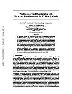
Identifying Rare and Subtle Behaviours: A Weakly Supervised Joint Topic Model Timothy M. Hospedales, Jian Li, Shaogang Gong, Tao Xiang Abstract—One of the most interesting and desired capabilities for automated video behaviour analysis is the identification of rarely occurring and subtle behaviours. This is of practical value because dangerous or illegal activities often have few or possibly only one prior example to learn from, and are often subtle. Rare and subtle behaviour learning is challenging for two reasons: (1) contemporary modeling approaches require more data and supervision than may be available and (2) the most interesting and potentially critical rare behaviours are often visually subtle – occurring among more obvious typical behaviours or being defined by only small spatio-temporal deviations from typical behaviours. In this paper we introduce a novel weakly-supervised joint topic model which addresses these issues. Specifically we introduce a multi-class topic model with partially shared latent structure and associated learning and inference algorithms. These contributions will permit modeling of behaviours from as few as one example, even without localisation by the user and when occurring in clutter; and subsequent classification and localisation such behaviours online and in real time. We extensively validate our approach on two standard public-space datasets where it clearly outperforms a batch of contemporary alternatives. Index Terms—Probabilistic model, behaviour analysis, imbalanced learning, weakly supervised learning, classification, visual surveillance, topic model, Gibbs sampling

F

1

I NTRODUCTION

The general objective of computer vision based analysis of behaviour in busy public spaces has been much studied in the last decade, both because of the tremendous associated research challenges and strong application demand for algorithms which can work on real-world data. One important problem without a good existing solution is that of learning to detect and classify behaviors of semantic interest in busy public spaces which may be both rare and subtle. The relevance of this problem is clear as for most surveillance scenarios, the behaviours of greatest semantic interest for detection are often rare (for example civil disobedience, shoplifting, driving offenses) and (possibly intentionally) visually subtle compared to more obvious ongoing behaviour in a busy public space. These are also the reasons why this problem is challenging and unsolved: rare behaviours by definition have few examples to learn from and moreover, the most interesting rare behaviours are visually subtle and hard to identify. Consider for example the scene in Fig. 1, the (rare) traffic violations illustrated here are simple, but hard to pick out amongst the numerous ongoing typical behaviours. This also highlights the need for effective classification, as different rare behaviours may indicate situations of different severity (e.g., a turn violation vs a collision) requiring different responses. Our approach is motivated by the modes of failure of existing methods in meeting the identified challenge of rare behaviour classification in busy spaces. Supervised learning methods can potentially learn to classify The authors are with the School of Electronic Engineering and Computer Science, Queen Mary University of London, E1 4NS, UK. Email: {tmh,jianli,sgg,txiang}@eecs.qmul.ac.uk

behaviours [1], [2], but perform poorly in our case where the target class has few examples. Moreover, the manual effort required to label training data by localising rare behaviors in space and time may be prohibitively costly. For this reason much recent work has focused on unsupervised density estimation methods [3], [4], [5], [6] which learn generative models of normal behaviour and can thereby potentially detect rare behaviours as outliers. However, there are serious limitations: i) their performance is sub-optimal due to not exploiting the few positive examples that may be available; ii) as outlier detectors they are not able to categorize different types of behaviour; and iii) they fail dramatically in cases where the target behaviour is non-separable in feature space. That is, if observation or pre-processing limitations mean that a rare behaviour is indistinguishable in the chosen feature space from some typical behaviour, then outlier detectors will not be able to detect it without a prohibitive cost in false positives. In this study we first consider learning behaviour models from rare and subtle examples in busy scenes. By rare behaviour, we mean as few as one example, i.e., one-shot learning. By subtle we mean little visual evidence: there may be few video pixels associated with the behaviour and/or few pixels differentiating a rare behaviour from a typical one. We moreover eliminate the prohibitive labeling cost of traditional supervised methods by performing this task in a weakly supervised context – in which the user need not explicitly locate the target behaviours in training video. Secondly, we consider classification and localisation of learned behaviours in test video. To address these problems we introduce a new weakly supervised joint topic model (WS-JTM) and associated learning algorithm which jointly learns a

2

(a) Typical

(b) Left-turn

(c) Right-turn

Figure 1. Surveillance video usually contains numerous examples of (a) typical behaviours and sparse examples of rare behaviours (b) and (c). Rare behaviours (red) also usually co-occur with other typical behaviours (yellow).

model for all the classes using a partially shared common basis. The intuition behind this approach is that well learned common behaviors implicitly highlight the few features relevant to the rare and subtle behaviours of interest, thereby permitting them to be learned without explicit supervision. Moreover the shared common basis helps to alleviate the statistical insufficiency problem in modeling rare behaviors. Importantly, we also introduce a fast inference algorithm for WS-JTM. These innovations allow for the first time learning behaviours which are both rare, subtle and not explicitly localised in the training data; and subsequent real-time classification and localisation of rare behaviors in test video. Terminology: Before continuing, we summarise our terminology as some terms are used in multiple ways by related literature. Visual words refer to extracted pixellevel features used as input to the model. A behaviour is of semantic significance to a human, and may be represented by one or more activities or topics in the model, each of which corresponds to a learned set of visual words. Clips or documents refer to short segments of video. Finally, class is a clip level attribute which indicates whether the clip includes a particular behaviour.

2

R ELATED W ORK

Computer vision based behaviour analysis approaches vary along three broad axes: input representation, behaviour model and learning approach. Input representations are typically either object centric – in the form of tracks [7], [8], [9]; or pixel centric – in the form of low level pixel [10], texture [11] or optical flow [12], [13], [3], [14], [15] data. Trajectory based representations allow behaviours such as typical paths to be cleanly modelled by simple clustering [16]; and events readily defined in terms of individual trajectories such as counter-flow [17] or u-turns [16] to be detected. These models, however, depend crucially on the reliability of the underlying tracker which can be compromised in many realistic situations of interest including crowded scenes with many targets, inter-object occlusion, low video resolution and low frame-rates (discontinuous movement). To improve robustness to missed detections and broken tracks, many recent studies have processed low-level image data directly [18], [19], [4], [10], [5], [3], [15]. To deal with the relatively impoverished input features and

to model more complex multi-object behaviours, these studies have focused on developing more sophisticated statistical models than the relatively simple clustering techniques [16] used for track data. Typical approaches include Gaussian mixture models (GMMs) [15], Dynamic Bayesian Networks (DBNs) such as a Hidden Markov Models (HMM) [18], [19], [20] or probabilistic topic models (PTMs) [4] such as Latent Dirichlet Allocation (LDA) [21] or extensions [3]. DBNs are natural for modeling dynamics of behaviour [1], [20], [19], [18]. However, explicit DBN models of multiple object behaviours are often exponentially costly in the number of objects, rendering them intractable for the busy scenes of interest. To overcome the problems of computational complexity and robustness in DBNs, PTMs [21] were borrowed from text document analysis. In the text domain, these models represent documents as a bag of words via a unique mixture of intermediate topics; each of which defines a distribution over words. Applied to behaviour analysis, PTMs represent video clips as a unique mixture of activities; each of which defines a distribution over visual words [3], [5], [4], [12]. There are two drawbacks however: inference in many PTMs is computationally expensive (preventing the desired usage for real-time monitoring of events in a public space) and they are unsupervised – limiting their accuracy and precluding classification of behaviors. Our proposed WS-JTM addresses the typical PTM weakness of inference speed and exploits weak supervision. Unsupervised detection of unusual or abnormal behaviours has recently been a topical problem in behaviour analysis to which statistical models including DBNs [1], [20], [19], PTMs [4], [3] and hybrids [5], [12] have been applied. In each case a generative model of typical scene statistics is learned and abnormal behaviours are then detected if they have low likelihood under the learned model. This approach has the advantage of fully automatic operation and no supervision requirements. However it also has crucial limitations. In addition to limited accuracy, constraints on data separability and inability to categorize identified earlier, there is also a visual subtlety constraint. Unusual behaviours of genuine interest are often visually subtle (possibly intentionally) compared to more obvious and numerous ongoing typical behaviours. A video containing a subtle unusual behaviour may still be typical on average and many sophisticated outlier detectors will fail [3], [5]. Alternatively, supervised classification methods have also been applied to behaviour analysis [1], [2]. These can perform well given sufficient and unbiased labeled training data, and unlike unsupervised methods, they can deal with non-separable data and classify behaviours. However, they are intrinsically limited in modeling rare behaviours due to their absolute sparsity and relative imbalance [22] to typical classes, making it difficult to build a good decision boundary. Moreover, there are still the problems of subtlety: (i) the vast majority of features in a rare class video may be typical due to ongoing

3

typical behaviours and (ii) since subtle rare behaviours often have much in common with typical behaviours, there may be few features upon which to discriminate them. These problems mean that even if large amounts of training data were available, conventional classifiers will fail without very specific and expensive supervision localizing each behaviour of interest in space and time. In contrast, WS-JTM is capable of learning from sparse and weakly labeled training examples. Other domains also encounter practical problems in providing full supervision, for example visual object recognition, where generating training data requires tedious object segmentation. To this end, weaklysupervised (WSL) [23], [24] and in particular multiinstance learning (MIL) [25], [26] have been exploited. Labels are provided at image level and weaklysupervised algorithms simultaneously learn to localise and classify objects of interest. Typical MIL algorithms are however unsuited to modeling behavior because they treat instances independently within each bag. In contrast our approach builds a topic model to represent the correlations that define complex behaviors. MIL approaches [25], [26] moreover rely on exploiting large quantities of data (positive instances are not assumed to be rare in absolute number). Our task of learning both rare and subtle behaviors is therefore harder still. We address this challenge by exploiting background class modelling to good effect: rare behaviours are implicitly identified by their deviation from normality without explicit supervised localization. Thus we achieve rare and subtle behaviour learning where existing methods require more specific supervision (typical supervised classifiers) or numerous examples (typical WSL or MIL). Other related modeling efforts to ours should be explicitly contrasted: supervised latent Dirichlet allocation (sLDA) [27], delta latent Dirichlet allocation (∆LDA) [28], and one-shot constellation models [29], [30]. ∆LDA [28] is a weakly supervised topic model applied to understanding bugs in computer software. Our WS-JTM is partially inspired by ∆LDA and improves on it in the following ways: (i) ∆LDA is binary while WS-JTM models multiple classes; (ii) ∆LDA is mathematically ill defined. By constraining Dirichlet parameters to be zero, the likelihood of a ∆LDA model cannot be computed (which prohibits parameter learning etc). WS-JTM provides a multiple-model formulation with well defined likelihoods; (iii) ∆LDA requires hand-tuned parameters while WS-JTM exploits hyperparameter learning; and (iv) ∆LDA is defined only for learning – lacking an inference algorithm to classify new data. We show how to perform efficient inference in WS-JTM, permitting real-time behaviour analysis. sLDA [27] learns a topic model with the additional objective of finding topics that help to discriminate data classes. We will demonstrate however that it fails in our subtle and rare behaviour context due to making no provision for the imbalanced [22] nature of the problem. Finally, constellation models for object recognition [23] have been learned in a rare

class context [29], [30] by transferring prior knowledge learned from common classes to rare classes [31]. There are a few contrasts to be made here. Firstly, this approach is synergistic to ours in that we do not currently exploit transfer learning, but could potentially do so to further improve performance. Secondly, object recognition is easier than our problem in that (i) it is static, while behaviors are temporally extended; and (ii) it is not subtle: Target objects are present in every positive image, tend to be the main foreground component of the image, and tend to preferentially attract the pre-processing interestpoint detectors. All of these points greatly reduce the difficulty of the weak supervision aspect of the object recognition problem compared to our subtle behaviours, which are potentially visible in a minority of pixels for a minority of frames within a training clip. Our joint modelling approach, which implicitly localises target class features, is therefore more appropriate than transfer learning [29], [30] to model rare and subtle behaviours.

3

V IDEO F EATURE R EPRESENTATION

Our approach uses quantized low-level motion and position features to represent video, as adopted by [3], [5], [14]. For each pixel, we compute an optical flow vector using the Lucas-Kanade algorithm. Next, we spatially divide a scene into Na × Nb non-overlapping square cells each of which covers H × H pixels. For each cell, we compute a motion feature by averaging all optical flow vectors in the cell. Finally, each cell motion feature is quantized into one of Nm directions. We note that discretization necessarily imposes a loss of spatial and directional fidelity [15]. This loss can be reduced by increasing discretization resolution at a cost of increased training data requirement and computation time. We found it straightforward to set a suitable discretization such that no object was small enough that its motion was missed in the discrete encoding. After spatial and directional quantization, we obtain a codebook V of Nv = Na × Nb × Nm visual words: v V = {vf }N f =1 . This codebook is used to index all the cell motion features and establish a bag-of-words representation of video. To create visual documents, we temporally segment a video into Nd non-overlapping clips and the visual words from each clip compose the corresponding visual document. Throughout this paper, we denote a d corpus of Nd documents as X = {xj }N j=1 in which each Nj document xj is a bag of Nj words xj = {xj,i }i=1 .

4 W EAKLY -S UPERVISED ELING (WS-JTM)

J OINT TOPIC M OD -

Our model builds on Latent Dirichlet Allocation (LDA) [21]. Applied to unsupervised behaviour modeling [32], [5], [3], LDA learns a generative model of video clips xj (Fig. 2(a)). Each visual word xj,i in a clip is distributed according to a discrete distribution p(xj,i |φyj,i , yj,i ) with parameter Φ indexed by its (unknown) parent activity

4 ε

α(0)

α(1)

α

c=0

θ

y

θ

c=1

y

x

y

x

x Nj

Nj Nd

ϕ

θ

Typical Clips

β Nt

(a) LDA

Nj c=0 Nd

Rare Class 1

ϕ

c=1 Nd

β Nt

(b) WS-JTM

Figure 2. (a) LDA [21] and (b) our WS-JTM graphical model structures (only one rare class shown for illustration). Shaded nodes are observed.

yj,i . Activities are distributed as p(y|θ j ) according to a per-clip Dirichlet distribution θ j . Learning in this model effectively clusters co-occurring visual words in X and thereby discovers regular activities y in the dataset. This activity based representation of video can facilitate, e.g., querying and similarity matching by searching for clips containing a specified activity profile, or detecting unusual clips by their low likelihood p(x). It also promotes robustness by permitting similarities between clips to be discovered even with few visual words in common. 4.1

composed from a mixture of activities from T0 (Fig. 2(b), left), while clips x ∈ Xc of each rare class c are composed from a mixture of activities T0,c , T0 ∪ Tc (Fig. 2(b), PNc c right). So while there are Nt = c=0 Nt activities in total, each clip may be explained by a class specific of subset of activities – in proportions and locations which are unknown and to be determined by the algorithm. By way of contrast to standard LDA which uses a fixed (and usually uniform) activity hyperparameter α, in WSJTM the dimension of the per-clip activity proportions θ and prior α are now class dependent. So if α(0) are the typical activity priors, α(c) the priors unique to class c, and α , [α(0), α(1), .., α(Nc )] is the list of all the activity priors; then typical clips c = 0 are generated with parameters αc=0 , α(0) and rare clips c > 0 with αc , [α(0), α(c)]. In this way, we explicitly establish a shared space between common and rare clips which will enable us to differentiate their subtle differences, overcome the problem of sparse rare behaviors and improve classification accuracy. We can summarize the generative process of WS-JTM as follows: 1) For each activity k, k = 1, · · · , Nt ; a) Draw a Dirichlet word-activity distribution φk ∼ Dir(β); 2) For each clip j, j = 1, .., Nd ; a) Draw a class label cj ∼ Multi(ε); b) Choose the shared prior αc=0 , α(0) or αc>0 , [α(0), α(c)]. c) Draw a Dirichlet class-constrained activity distribution θ j ∼ Dir(αc ); d) For observed words i = 1..Nwj in clip j: i) Draw an activity yj,i ∼ Multi(θ j ); ii) Sample a word xj,i ∼ Multi(φyj,i ). The probability of variables {xj , yj , cj , θ j } and parameters Φ given hyper-parameters {α, β, } in a clip j is:

Model Structure

In contrast to standard LDA, WS-JTM (Fig. 2(b)) has two objectives: (1) learning robust and accurate representations for both typical behaviours which are statistically sufficient and a number of rare behaviour classes of which few (non-localised) examples are available; and (2) classifying clips in test data using the learned model. These will be achieved by jointly modelling the shared aspects of typical and rare clips. d Given a database of Nd clips X = {xj }N j=1 , assume that Nc X can be divided into Nc + 1 classes: X = {Xc }c=0 with c Nd clips per class. The crucial assumption we will make in WS-JTM – which will permit rare behaviour modeling in busy scenes – is that clips X0 of class 0 contain only typical activities while class c > 0 clips Xc may contain both typical and class c rare activities. We enforce this modelling assumption by partially switching the generative model of clip according to its class (Fig. 2(b)). Specifically, let T0 be the Nt0 element list of typical activities and Tc be the Ntc element list of rare activities unique to each rare behaviour c. Then typical clips x ∈ X0 are

p(xj , yj , θ j , Φ, cj |α, β, ε)

=

Nt Y

p(φt |β)

t=1 j

·

Nw Y

p(xj,i |yj,i , φyj,i )p(yj,i |θ j )p(θ j |αcj )p(cj |ε). (1)

i=1

The probability p(X, Y, c|α, β, ) of a video dataset X = Nd Nd d {xj }N j=1 , Y = {yj }j=1 , c = {cj }j=1 can be factored as: p(X, Y, c|α, β, )

p(X|Y, β)p(Y|c, α)p(c|ε). (2)

=

Here, the first two terms are products of Polya distributions over activities k and clips j respectively: ˆ p(X|Y, β)

= =

p(X|Y, Φ)p(Φ|β)dΦ, Q Nt Y Γ(Nv β) v Γ(nk,v + β) Q P , v Γ(β) Γ( v nk,v + β)

k=1

(3)

5

ith visual words in clip j ith topic/activity in clip j Class of clip j Word probability vector for topic y Activity probability vector for clip j Dirichlet word prior Dirichlet activity prior vector Typical activity prior vector Rare activity c prior vector

xi,j = 1...Nv yi,j = 1...Nt cj = 1...Nc φy θj β α α(0) α(c), c > 0

Iteration of Eq. (5) draws samples from the posterior p(Y|X, c, α, β). Y−j,i denotes all activities excluding yj,i ; ny,x denotes the counts of feature xj,i being associated to activity yj,i ; nj,y denotes the counts of activity yj,i in clip j. Superscript −j, i denotes counts excluding item (j, i). In contrast to standard LDA (Fig. 2(a)), the topics which may be allocated by our joint model (Fig. 2(b)) are constrained by clip class c to be in T0 ∪Tc . Activities Tc=0 will be well constrained by the abundant typical data. Clips of some rare class c > 0 may use extra activities Tc in their representation. These will therefore come to represent the unique aspects of interesting class c. Each sample of activities Y entails Dirichlet distributions over the activity-word parameter Φ and per-clip activity parameter θ j - p(Φ|X, Y, β) and p(θ j |yj , cj , α). These can then be point-estimated by the mean of their Dirichlet posteriors:

Table 1 Summary of model parameters

Nd ˆ Nc Y Y c

p(Y|c, α)

=

p(yj |θ j )p(θ j |α, cj )dθ j ,

c=0 j=1

P Q Ndc Nc Y Y Γ( k αk ) k Γ(nj,k + αk ) Q P = . k Γ(αk ) Γ( k nj,k + αk ) c=0 j=1

(4)

where nk,v and nj,k indicate the counts of activity-word and clip-activity associations and k ranges over activities T0,c permitted by the current document class cj . For convenience, Table 1 summarizes the model parameters. We next show how to learn a WS-JTM model (training) and use the learned model to classify new data (testing). For training, we assume weak supervision in the form of labels cj , and the goal is to learn the model parameters {Φ, α, β}. For testing, parameters {Φ, α, β} are fixed and we infer the unknown class of test clips x∗ . 4.2 WS-JTM Learning We first address learning our WS-JTM from training data {X, c}. This is non-trivial because of the correlated unknown latents {Y, θ} and parameters {Φ, α, β}. The correlation between these unknowns is intuitive as they broadly represent “which activities are present where” and “what each activity looks like”. A standard EM approach to learning with latent variables is to alternate between inference – computing p(Y|X, c, α, β); and hyperparameter estimation – optimizing {α, β} ← P argmax Y log p(X, Y|c, α, β)p(Y|X, c, α, β). Neither of α,β

these sub-problems have analytical solutions in our case, but we develop approximate solutions for each in the following two sections. 4.2.1 Inference Similarly to LDA, exact inference in our model is intractable, but it is possible to derive a collapsed Gibbs sampler [33] to approximate p(Y|X, c, α, β, ). The Gibbs sampling update for the activity yj,i is derived by integrating out the parameters Φ and θ in its conditional probability given the other variables:

−j,i v (ny,v

+ β)

n−j,i j,y + αy −j,i k (nj,k

P

nj,k + αk θˆj,k = P . k (nj,k + αk )

(7)

α,β

framework is still intractable because of the sum over Y with exponentially many terms. However, we can use Ns Gibbs samples Ys ∼ p(Y|X, c, α, β) drawn during inference (Eq. (5)) to define a Gibbs-EM algorithm [34], [35] which approximates the required optimization as {α, β} ← argmax α,β

Ns 1 X log (p(X|Ys , β)p(Ys |c, α)) . (8) Ns s

We learn β by substituting Eq. (3) into Eq. (8) and maximizing for β. The gradient g with respect to β is g

=

d 1 X log p(X|Ys , β), dβ Ns s

=

1 XX Nv Ψ(Nv β) − Nv Ψ(β) Ns s k

! X

Ψ(nk,v + β) − Nv Ψ(nk,· + Nv β) , (9)

v

p(yj,i |Y−j,i , X, c, α, β) ∝ P

(6)

4.2.2 Hyperparameter Estimation The Dirichlet prior hyperparameters α and β play an important role in governing the activity-word p(X|Y, β) and clip-activity p(Y|c, α) distributions. β describes the prior expectation about the the “size” of the activities - how many visual words are expected in each. More crucially, elements of α describe the relative dominance of each activity within a clip of a particular class. That is, in a class c clip, how frequently are observations related to rare activities Tc expected compared to ongoing normal P activities T0 ? Direct optimization {α, β} ← argmax Y log p(X, Y|c, α, β)p(Y|X, c, α, β) in an EM

+ n−j,i y,x + β

nk,v + β φˆk,v = P v (nk,v + β)

+ αk )

.

(5)

where nk,v is the matrix P of topic-word counts for each E-step sample, nk,· , v nk,v , and Ψ is the digamma function. This leads [36], [34] to the iterative update:

6

4.3 β new

P P P s k v Ψ(nk,v + β) − Nt Nv Ψ(β) P P =β . (10) Nv s ( k Ψ(nk,· + Nv β) − Nt Ψ(Nv β))

Compared to β, learning the hyperparameters α is harder because they are class-dependent. A simple approach is to define a completely separate αc for each class and maximize p(Yc |αc ) independently for each c, but this leads to poor estimates for the frequency of typical activities from the point of view of each rare class. This is because the rare class αc>0 parameter updates would take into account only a few (possibly 1) clips to constrain the typical elements of αc although much more data about typical activity is actually available. To alleviate the problem of statistical insufficiency in learning α we exploit the novel shared-structure approach of WS-JTM (Section 4.1 and Fig. 2(b)) to develop a new learning algorithm. Specifically, by defining αc , [α(0), α(c)] we established a shared space of typical activities α(0) for all classes. This will alleviate the sparsity problem by allowing data from all clips to help constrain these parameters. In the following, we will use K 0 to represent the indices into α of the Nt0 typical activities; K c to represent the Ntc indices of the rare activities in class c and K c,0 = K 0 ∪ K c both typical and class c activities. Hyperparameters α are learned by fixed point iterations (derived in Appendix A) of the form: a (11) αknew = αk . b For typical for typical activities k ∈ K 0 the terms are: a=

Nd Ns X X

(Ψ(nj,k + αk ) − Ψ(αk )) ,

(12)

s=1 j=1 c

b=

Nd  Ns X Nc X X

 0,c 0,c Ψ(n0,c j,· + α· ) − Ψ(α· )

s=1 c=1 j=1 0

+

Nd Ns X X

(13)

P P 0,c 0 where α·0 , , , 0 αk , nj,· k∈K k∈K 0 nj,k , α· P P 0,c α , n , n . For class c rare activities j,· k∈K 0,c k k∈K 0,c j,k k ∈ K c the terms are: c

=

Nd Ns X X

(Ψ(nj,k + αk ) − Ψ(αk )) ,

(14)

s=1 j=1 c

b

=

In this section we address inference for unseen video given the learned model {α, Φ} from Section 4.2. Specifically, we classify each test clip x∗ , i.e. determine if it is better explained as a clip containing only typical activities (c = 0), or typical activities and some rare activities c, (c > 0). Note that in contrast to the E-step inference problem of Section 4.2.1 where we computed posterior of activities y via Gibbs sampling; we are now computing the posterior class c which will require the harder task of integrating out activities y. In this section we will show how to perform this integration efficiently. The desired class posterior is given by p(c|x∗ , α, ε, Φ) ∝ p(x∗ |c, α, Φ)p(c|ε), (16) ˆ X p(x∗ |c, α, Φ) = p(x∗ , y|θ, Φ)p(θ|α)dθ (17) y

The challenge is that of accurately and efficiently computing the class-conditional marginal likelihood in Eq. (17). Efficiently and reliably computing the marginal likelihood in topic models is an active research area [37], [38] due to the intractable sum over correlated y in Eq. (17). We take the view of [37], [38] and define an importance sampling approximation to the marginal likelihood: 1 X p(x∗ , ys |c) , ys ∼ q(y|c), (18) p(x∗ |c) ≈ S s q(ys |c) where we drop conditioning on the parameters for clarity. Different choices of proposal q(y|c) induce different estimation algorithms. The (unknown) optimal proposal qo (y|c) is p(x∗ , y|c). We Q can develop a mean field approximation qmf (y|c) = i qi (yi |c) with minimal KullbackLeibler divergence to the optimal proposal by iterating   X qi (yi |c) ∝ αyc + ql (yl |c) φˆyi ,xi . (19) l6=i


Ψ(n0j,· + α·0 ) − Ψ(α·0 ) ,

s=1 j=1

a

WS-JTM Online Classification

Nd  Ns X X

 0,c 0,c Ψ(n0,c j,· + α· ) − Ψ(α· ) .

(15)

s=1 j=1

Iteration of Eq. (10) and Eqs. (11)-(15) estimates the hyperparameters {α, β} and is used periodically during sampling Eq. (20) to complete the Gibbs-EM algorithm.

The new importance sampling proposal in (Eq. (19)) results in much faster and more accurate estimation of the marginal likelihood (Eq. (17)) than the standard approach [39], [37] of using posterior Gibbs samples. The latter results in the harmonic mean approximation for the likelihood [39], [37] and suffers from (i) requiring a (slow) Gibbs sampler at test time (prohibiting online computation) and (ii) the high variance of the harmonic mean estimator (making classification inaccurate). The new proposal is crucial for us because classification speed and accuracy is determined by the speed and accuracy of computing marginal likelihood (Eq. (17)). In summary, to classify a new clip, we use the importance sampler defined in Eqs. (18) and (19) to compute the marginal likelihood (Eq. (17)) for each class c (i.e. typical 0, rare 1,2,...) and hence the class posterior for that clip (Eq. (16)). Interestingly, classification in our

7

framework is essentially a model selection [40] computation. We must determine (in the presence of numerous latent variables y) which generative model provides the better explanation of the data: a simple one involving only typical behaviour (Fig. 2(b), left); or one of a set of more complex models involving both typical and rare behaviours (Fig. 2(b), right). The simpler typical only model is automatically preferred by Bayesian Occam’s razor [40]; but if there is any evidence of a particular rare activity, the corresponding complex model is uniquely able to allocate the associated rare topic and thereby obtain a higher likelihood. 4.4

WS-JTM Localisation

Once a clip has been classified as containing a particular rare behavior, we may moreover be interested in localising the behaviour of interest in space and time. In notable contrast to unsupervised outlier detection approaches to rare behavior detection [3], [5], WS-JTM provides a principled means to achieve this. Specifically, for a test clip j of type c, we determine its activity profile ˆ with Gibbs sampling by iterating: p(yj |xj , c, α, Φ) ˆ p(yj,i |y−j,i , xj , c, α, Φ) ∝ φˆy,x P

n−j,i j,y + αy

−j,i k (nj,k

+ αk )

.(20)

We then list the visual words i for which the corresponding sampled activity yj,i is a class c rare activity, i.e., I = {i} s.t. yj,i ∈ Tc . The indices of these visual words I within the clip provide an approximate spatio-temporal segmentation of the behaviour of interest. Because parameters α and Φ are already estimated, this Gibbs localisation procedure needs many fewer iterations than the initial model learning and is hence much faster.

5 5.1

E XPERIMENTS Classifying Simulated Data with Ground Truth

In this section, we apply our proposed framework to a simulated dataset. This serves three purposes: to illustrate the mechanisms of our model; to validate its correct behaviour on data which is non-trivial yet has known ground truth; and to provide insight into its properties compared to other standard approaches as a function of input sparseness which we can control precisely here. The experiment is illustrated in Fig. 3. We created eleven 2D patterns {φy } to represent ground-truth activities, in which eight (bars) were typical and three (stars) were rare. Following the generative process in Section 4.1, we sampled training documents as follows. First, we generated 500 documents with only typical activities (Fig. 3, 2nd row, middle); and 500 documents for each rare class by sampling both the 8 typical activities and corresponding rare activity (Fig. 3, 2nd row, right). We assumed 500 typical documents and varied the number of rare documents for training from 1 to 500, resulting in training set sizes from 503 to 2000. We

also generated a separate test set with 50 documents per class. All Dirichlet hyperparameters α were set to 0.5 and all documents contained 1000 tokens. One-shot learning: We trained our WS-JTM with 500 typical documents and one from each rare class, i.e., one-shot learning. The 11 learned activities are shown in Fig. 3(c). The model learns a fairly good representation of each rare activity despite having only one noisy and non-localised example each (Fig. 3(b)). This is because it is able to leverage the shared structure and the typical activity representation which is better constrained by the more numerous typical documents to implicitly localise the rare patterns in the training set. Next we applied the learned model to classify test documents. Fig. 3(d) shows some test document examples in which each row illustrates a class. The classification accuracies are shown in the confusion matrix in Fig. 3(e). Quantifying the effect of data sparsity: To illustrate the challenge involved in rare-class learning and validate our contribution over existing state of the art models, we performed a second experiment in which we varied the number of documents in each rare class from 1 to 500. We compared against the following methods: 1) Supervised LDA (sLDA [41], [42]): A supervised topic model classifier. It jointly learns a topic model for the data and a topic profile-based classifier. We utilized the implementation of [42] and set the number of topics to 11. 2) LDA Classifier (LDA-C): Treating LDA as a classconditional generative model, we learned a separate model [39], [21] for each class of documents with 8 topics per class. Dirichlet hyperparameters α and β were learned using [43]. For classification, we computed the test document likelihood under each LDA model class using importance-sampling method proposed in Section 4.3 and then calculated the class posterior assuming equal priors. 3) Multi-Class SVM (MC-SVM): A Gaussian kernel classifier was trained directly on visual word counts with hyperparameters {C, γ) optimized by grid search. To account for dataset imbalance, the misclassification cost parameter Cc was weighted on a per-class basis according to the inverse proportion of that class in each training dataset [22]. The classification results are shown in Fig. 4. Given only 1 or few rare training documents, all existing approaches performed very poorly. Specifically existing methods classify most test documents as typical, resulting in average accuracy around 30%. In contrast, the proposed WS-JTM achieved average accuracy of 58% even with one-shot learning. Existing methods approach but do not outperform WS-JTM as the numbers examples per class becomes balanced. This key result shows that for the important task of weakly supervised rare-class learning and classification, WS-JTM provides a decisive advantage over existing techniques.

8

8 typical topics

3 rare topics

(a) Topic groundtruth

Sampling documents

(b) Training documents 1 document for each rare class

Train model

500 typical documents

(c) Learned topics 3 rare topics

8 typical topics

Classification

(e) Classification accuracy

(d) Unseen documents Figure 3. Illustration and validation of WS-JTM using synthetic data.

5.2

Mean classification accuracy (%)

70

60

50

40

WS−JTM LDA−C sLDA MC−SVM

30

20 1

2

5 10 50 100 200 Number of documents in each rare class

500

Figure 4. Synthetic data classification performance as a function of rare-class example sparsity. One-shot learning corresponds to the y-axis. Our WS-JTM exhibits dramatically superior performance in the low data domain.

Classifying Real-World Rare Behaviors

We evaluate our WS-JTM on classifying rare behaviours in two real-world video datasets: the MIT dataset [3] (30Hz, 720 × 480 pixels, 1.5 hour) and the QMUL dataset [4] (25Hz, 360 × 288 pixels, 1 hour). Both scenes featured numerous objects exhibiting complex behaviours concurrently. Figs. 5(a) and (d) illustrate the behaviours that typically occur in each scene. Unlike many existing studies [3], [4], [5], [12] which focus on learning typical behaviours and their concurrence or temporal correlation, our objective is to learn to classify rare behaviours which are of particular interest to visual surveillance applications. In the MIT dataset (Fig. 5(a) and (b)), we are interested in the illegal left-turn and right-turn at different locations of the scene (red arrows). In the QMUL dataset (Fig. 5(a) and (b)), our targets are the U-turn at the center of the scene, and the near-collision situation in which horizontal flow vehicles drive into the junction (red arrow) before turning traffic finishes. To create a visual word vocabulary, we followed the procedure in Section 3. The videos were spatially quantized into 72 × 48 cells (MIT) and 72 × 57 cells (QMUL)

9

(a) Typical

(b) Left-turn

(c) Right-turn

(d) Typical

(e) U-turn

(f) Collision

Figure 5. Example typical and rare behaviours in the (a)(c) MIT and (d)-(f) QMUL surveillance datasets.

Figure 6. Typical activities learned from the MIT dataset. Red: Right, Blue: Left, Green: Up, Yellow: Down.

Table 2 Number of clips used in the experiments. Total Train Test Total Train Test

MIT Rare 1 (26) 1, 2, 5, 10 16 QMUL Typical (200) Rare 1 (12) 100 1, 2 100 10 Typical (300) 200 100

Rare 2 (28) 1, 2, 5, 10 18 Rare 2 (5) 1, 2 3

(a) Rare 1: Left Turn

(b) Rare 2: Right Turn

Figure 7. One shot learning of rare activities: MIT dataset. respectively, and motion direction in each cell quantized into 4 orientations (up, down, left, right) resulting in codebooks of 13824 and 16416 words respectively. Each dataset was temporally segmented into non-overlapping video clips of 300 frames each. We manually labeled the clips into three classes: typical, rare 1 and rare 2, according to which, if any, rare behaviour existed in each clip. The total available numbers of clips for each behaviour class are detailed in Table 2. Throughout our experiments, we varied the number of training clips for each rare class while keeping constant the number of typical training clips and testing clips for all classes. In each case we used 20 typical activities and one activity per rare class for ease of visualisation. 5.2.1 Learning Activity Models of Rare Behaviours We first evaluate the proposed WS-JTM on learning activity representations for both typical and rare behaviours. In this experiment we assume a one-shot learning condition, i.e. the training corpora contain only 1 clip per rare behaviour (see Table 2). We apply our Gibbs-EM learning algorithm proposed in Section 4.2 for 2000 iterations of burn-in with hyper-parameter updates every 100 iterations and then draw five samples from the posterior (Eqs. (20)-(7)). All quantitative results are averages of three folds of cross validation MIT dataset. The dominant visual words (large p(x|φy )) are used to illustrate the some of the learned typical and rare activities φy . The illustrative typical activities in Fig. 6 show: pedestrians crossing (left column),

straight traffic (centre column) and turning traffic (right column). Fig. 7 shows that the learned rare activities match the examples in Figs. 5(b) and (c), and that these have generally been disambiguated from ongoing typical behaviours (Fig. 5(a)). This is despite (i) one-shot learning of rare behaviors; (ii) rare behavior subtlety in that more numerous typical behaviours were cooccurring overwhelmingly (Fig. 5(a)); and (iii) only small differences (potentially confusing similarity) between the some rare and typical activities (some arrow segments in Figs. 5(b) and (c) overlap those in Fig. 5(a)). QMUL dataset. In Fig. 8 some learned typical activities are illustrated including vertical traffic (left column), horizontal traffic (centre column) and turning traffic (right column). Learning rare activities in the QMUL dataset is harder because the scene is much busier, objects are highly occluded and motion patterns were frequently broken. For example, in the U-turn activity (Fig. 5(e)), vehicles often drive to the central area and wait for a break in oncoming traffic before continuing. Furthermore the rare activities are very subtle in that they are both composed mostly of visual words common to typical activities. Our results show that the proposed model is able to cope with such variations to learn descriptions of typical (Fig. 8) and rare (Fig. 9) behaviours. Dependence on data sparsity. The above results were based on one-shot learning. We also explored how additional rare-class examples can improve the learned behaviour representation. Fig. 10 illustrates the learned

10

typical

.89

.07

.04

typical

1.0

.00

.00

typical

1.0

.00

.00

typical

1.0

.00

.00

rare1

.19

.81

.00

rare1

1.0

.00

.00

rare1

1.0

.00

.00

rare1

1.0

.00

.00

rare2

.39

.00

.61

rare2

1.0

.00

.00

rare2

1.0

.00

.00

rare2

.99

typ

ra r

ra

typ ica l

ra

ra

typ ica l

ra

ra

ica l

e1

re

2

(a) WS-JTM

re 2

re 1

(b) sLDA

re 1

(c) LDA-C

.00

typ ica

re 2

.01

ra

ra

re

re

2

1

l

(d) MC-SVM

Figure 11. Classification confusion matrices after oneshot learning: MIT dataset. typical

.59

.26

.15

typical

1.0

.00

.00

typical

1.0

.00

.00

typical

1.0

.00

.00

rare1

.10

.90

.00

rare1

1.0

.00

.00

rare1

1.0

.00

.00

rare1

.97

.00

.03

rare2

.00

.33

rare2

1.0

.00

rare2

1.0

.00

rare2

1.0

.00

typ

ra

typ

ra

typ

ra

typ ica

ra

ica

l

re

.67

1

ra

re

2

(a) WS-JTM Figure 8. Typical activities learned from the QMUL dataset. Red: Right, Blue: Left, Green: Up, Yellow: Down.

(a) Rare 1: U-turn Figure 9. dataset.

(b) Rare 2: Near collision

One shot learning of rare activities: QMUL

rare behaviour models for an increasing number of examples. The simpler MIT dataset has more (10) rareclass examples available, and the learned behaviour representations are meaningful and accurate (Fig. 10(a)). The QMUL dataset (Fig. 10(b)) is more challenging and also has fewer available examples (5), so while the learned models captures the essence of the U-turn and collision behaviours they are not yet perfectly disambiguated from ongoing typical behaviour. 5.2.2 Classifying Rare Behaviours Online In this section we compare the classification performance of WS-JTM against contemporary approaches including sLDA, LDA-C and MC-SVM (as described in Section 5.1). In each case results are quantified in terms of the average classification accuracy for each class (i.e., the mean along the diagonal of the normalised confusion matrix). This ensures that errors of each type are weighted equally although the test data is imbalanced. One-shot learning. All models were learned with one clip from each rare class (see Table 2). For WS-JTM, we used the model learned in last section and classification was performed as described in Section 4.3. For sLDA, we learned 22 topics, to match the total number from WS-JTM. For LDA-C, we learned 8 topics per class. We

ica

l

re

.00

1

(b) sLDA

ra

re

2

ica

l

re

.00

1

ra

re

(c) LDA-C

2

.00

ra

re

l

1

re

2

(d) MC-SVM

Figure 12. Classification confusion matrices after oneshot learning: QMUL dataset.

assumed a uniform class prior p(c|ε) = 1/3 for each model. The resulting confusion matrices are shown in Fig. 11 (MIT dataset) and Fig. 12 (QMUL dataset). It is clear that the model selection approach to classification induced by WS-JTM and implemented by our importance sampler is qualitatively superior to other approaches. WS-JTM achieved 77% and 66% average classification rate on the MIT and QMUL datasets. The other approaches generally failed to classify instances of rare behaviours, interpreting almost every behaviour as typical resulting in their average accuracy of 33%. Thus far we have considered unbiased maximum likelihood classification. It is also possible to tune a classifier by applying a non-uniform threshold to the posterior p(c|x∗ ) for declaring the winning class, or equivalently by setting the class prior p(c|ε) non-uniformly. This is useful, for example, in many real-world applications with constant false alarm rate (CFAR) constraints. In such applications it is more important to control the rate at which false alarms distract the operator than to detect every instance of interest. In our context “false alarms” are instances of typical clips being classified as any of the rare behaviours. We therefore perform a CFAR evaluation by quantifying the average classification accuracy while varying the class label prior p(c|ε) parameter ε from 0 to 1, such that p(c = 0) = ε and p(c = 1) = p(c = 2) = (1 − ε)/2. This has the effect of biasing classification completely towards the typical behaviours for ε = 1 and towards the rare behaviours for ε = 0. Fig. 13 details the results. Circles indicate the points corresponding to the unbiased case p(c|) = 1/3 from Figs. 11 and 12. The sLDA implementation of [42] provides no posterior estimates, so we do not compare it here. Note that the curves which approach the top left (high classification accuracy with low false alarm rate) or which enclose a greater area should be considered better. WS-JTM’s accuracy curves enclose the greatest area (Fig. 13, legends) and more importantly, approach

11

5 Examples

1 Example

10 Examples

5 Examples

Rare 2: Collision

Rare 2: Right Turn

Rare 1: U-turn

Rare 1: Left Turn

1 Example

(a) MIT

(b) QMUL

Figure 10. Improvement of rare behaviour models with increasing number of training examples.

40 WS−JTM. (0.59) LDA−C (0.51) MC−SVM (0.54) 0.2

0.4 0.6 False Positives

(a) MIT dataset

0.8

1

50

40

0.2

0.4 0.6 False Positives

0.8

60

50

40

60

WS−JTM LDA−C sLDA MC−SVM

50

40

30

30

WS−JTM. (0.55) LDA−C (0.51) MC−SVM (0.37) 30 0

WS−JTM LDA−C sLDA MC−SVM

70

Mean classification accuracy

50

60 Mean classification accuracy

60

30 0

70

80

Mean classification accuracy (%)

Mean classification accuracy (%)

70

1

(b) QMUL dataset

Figure 13. Average classification accuracy achieved while controlling false alarm rate. Quantity in brackets indicates area under the curve. the top left with a dramatic margin over the other models. That is, performance is most clearly superior in the practically valuable domain of low false alarm rate. Dependence on Data Sparsity. We next increased the number of rare class training clips while fixing the typical clips (see Table 2). The average classification accuracy for all methods is reported in Fig. 14. In all cases, WSJTM produced superior classification accuracy. Comparing Fig. 14 to the classification results for synthetic data in Fig. 4 suggests that this dramatic improvement is because although we increased the number of rare class training examples, we still do not reach the domain where alternative methods begin to perform well (Fig. 4). This suggests that our WS-JTM is of great value for learning rare behaviours with 1 to 10 examples. Alternative models. To provide insight into our contribution, we consider why the alternative methods perform poorly on this classification task. The reasons come down to the challenges of learning from weakly-labeled subtle examples and from sparse imbalanced data which are better addressed by our model. MC-SVM failed to classify the clips directly from the visual word counts. The subtle and weakly-supervised nature of the problem (i.e., the few relevant features corresponding to the rare behaviours are unknown) is too challenging. Without provision for weakly-supervised learning, the ongoing

20 1

2 5 Number of documents in each rare class

(a) MIT dataset

10

20 1

2 Number of documents in each rare class

(b) QMUL dataset

Figure 14. Average classification accuracy given varying number of rare class training clips.

and more visually obvious typical behaviours dominate the classification. Multi-instance SVM learning could be considered [26] as an alternative, however as discussed earlier the simplifying assumptions made by this technique do not provide a good model for behaviors and moreover would require a change of representation to tracks or video cuboids. This would increase computational complexity and susceptibility to noise. sLDA [41], [42] learned a good typical behaviour model, but did not learn any topics corresponding to rare activities, preventing correct classification (Figure omitted due to space constraint). This seems to be due to sLDA balancing learning a good generative model of all the data with learning discriminative topics [42]. The benefit of spending topics to learn a better typical behaviour model overwhelms the benefit of spending them on learning a discriminative (rare activity) topic since there are so many more typical clips. In other words, sLDA fails due to the imbalanced data. In contrast, by reserving topics/activities for each rare behaviour (Fig. 2(b)), WS-JTM is much more successful at learning from imbalanced data. LDA-C learns an independent LDA model for each class. In the one-shot learning experiments (Figs. (11)(13)) this was insufficient to learn any clear activities from the rare data. In the experiment with the most data (MIT dataset, 10 examples per rare class) LDA-C was

4

4

1

2

3

4

5

6

7

8

(a) Learned topics using documents with only typical behaviours (a) Activities learned from 200 typical clips8 5 6 7

5

(a) Learned topics using documents with only typical behaviours 6 7 (a) Learned topics using documents with only typical behaviours

8

1

2

3

4

1

2

3

4

1

2

3

4

5

5

6 7 (b) Learned topics using documents in rare class 1 6 7 (b) Learned topics using documents in rare class 1 6 7 (b) Learned topics using documents in rare class 1

8

8

(b) Activities learned from 10 left turn clips8 5 1

2

3

4

1

2

3

4

1

2

3

4

5

5 5

6 7 (c) Learned topics using documents in rare class 2 6 7 (c) Learned topics using documents in rare class 2 6 7 (c) Learned topics using documents in rare class 2

8

8 8

(c) Activities learned from 10 right turn clips Figure 15. Activities learned by LDA-C.

able to learn a fair model of each class (Fig. (15)). The learned rare activities include the correct ones (Fig. 15(b), activity 7; Fig. 15(c), activity 5). However, there is a key factor which limits classification accuracy: each LDA model has to independently learn the ongoing typical activities. For example, Fig. 15(a), activity 1; Fig. 15(b), activity 5 and Fig. 15(c), activity 2 all represent “right turn from below.” By learning separate models for the same typical activities LDA-C introduces a significant source of noise. In contrast, by learning a single model for ongoing typical activities which is shared between all classes (Figs. (6) and (8)), WS-JTM avoids this source of noise. Moreover, by permitting the rare class models to leverage a well learned typical activity model, they can more accurately learn the rare activities (e.g., Fig. 15(b), activity 7 is noisier than the left turn in Fig. 10(a)). 5.2.3 Localising Rare Behaviours In this section we illustrate the ability of WS-JTM to approximately segment rare behaviours in space and time within a clip classified as rare. Fig. 16 illustrates examples of localising specific behaviours within correctly classified clips from the previous section. The brighter areas in each image are specific visual words which were labeled as corresponding the rare behaviour. The segmentation is rough, due to the noisy optical flow features

(b) Right turn

3

3

(c) U-turn

2

2

(d) Near Colision

1

1

(a) Left turn

12

Figure 16. Localisation of rare activities by WS-JTM.

and the MCMC based labeling. The bounding boxes of rare behaviour words (red rectangles) nevertheless provide a useful localisation in space and time. Note that in Fig. 16(d), the near-collision behaviour is intrinsically multi-object – being defined by the concurrent state of two traffic flows. The bounding box therefore contains elements of both contributing flows - the fire engine and the turning traffic. 5.3

Model Learning and Complexity Analysis

In this section we provide some additional intuition into our model’s function and validate the significance of two of our specific contributions, namely the hyperparameter estimation method proposed in Section 4.2.2 and the online inference method proposed in Section 4.3. Activity Profile Illustration. To provide additional insight into the mechanism of our model, Fig. 17 illustrates the topic profiles inferred for each of the clips shown earlier in Fig. 16. Clearly the model describes each clip in terms of a unique mixture (Fig. 17, yellow bars) of the learned typical activities (Figs. 6 and 8). The black lines in Fig. 17 illustrate the overall representation of each activity in the test datasets, within which the rareactivities (21 and 22) are a small proportion. In contrast, these particular rare class clips require a greater than average proportion (Fig. 17, red bars) of rare activities (Figs. 7 and 9) to be explained. Hyperparameter estimation. Thus far hyperparameters {αc } were learned using the method proposed in 4.2.2 – by allowing typical behaviour parameters α(0) to be shared across all classes. In this section, we compare this against two other simpler methods. In the first, all values in {αc } were set to 0.1 (constant). In the second, we naively learned {αc } for each class independently

13

0.3

0.25 Proportion

Proportion

0.25

80

0.2

0.2

0.15

0.15

0.1

0.1

0.05

0.05

65

60

55

50

45

Mean classification accuracy (%)

0.3

Mean classification accuracy (%)

0.4

0.35

Mean classification accuracy (%)

0.4

0.35

70 Mean Field Harmonic Mean

60

50

40

30

60

50

40

Mean Field Harmonic Mean

30

20

Mean Field Harmonic Mean

0

0

5

10

15

0

20

40 1

5

10

0.4

0.4

0.35

0.3

0.3

0.25

0.25 Proportion

Proportion

15

0.2

0.15

0.1

0.05

0.05

10

15

20

0

0

5

10

15

20

Activity

(c) QMUL: U-turn

(d) QMUL: Near collision

Figure 17. Estimated topic profile for rare clips from Fig. 16. Bar color indicates typical vs rare activities. Black line indicates the average profile over the entire dataset. 65

80

50

40

30 Shared Params Independent Params Constant Params

(a) Simulated

500

75

Mean classification accuracy

60

Mean classification accuracy

Mean classification accuracy (%)

70

5 10 50 100 200 Number of documents in each rare class

(b) MIT

10

10 1

2 Number of documents in each rare class

(c) QMUL

Importantly this is independent of the number of visual words Nw , so speed does not decrease with more scene activity as for Gibbs sampling. In practice training in our model (C implementation) proceeded at 11 and 2 FPS for the MIT and QMUL datasets respectively, while testing (matlab implementation) proceeded at 84 and 46 FPS respectively on a 3GHz PC.

0.15

0.1

2

2 5 Number of documents in each rare class

Figure 19. Classification accuracy using different methods for computing likelihoods of unseen documents.

0.2

Activity

20 1

20 1

20

(b) MIT: Right turn

0.35

5

500

Activity

(a) MIT: Left turn

0

5 10 50 100 200 Number of documents in each rare class

(a) Simulated 0

Activity

0

2

70

65

60

55

50 1

60

55

50 Shared Params Independent Params Constant Params

Shared Params Independent Params Constant Params 2 5 Number of documents in each rare class

(b) MIT

10

45 1

2 Number of documents in each rare class

(c) QMUL

Figure 18. Classification accuracy using different methods for estimating Dirichlet hyperparameters {αc }.

using only clips of the corresponding class and without a shared component. The results in Fig. 18 verify that our proposed algorithm performs best. As we discussed earlier, learning the hyperparameters independently is an especially poor choice for rare-class problems because (e.g., Fig. 18(a) and (b)) because their typical-class parameters are poorly constrained by the limited data. Likelihood computation. In the previous experiments, classification was performed via the likelihood computed by the algorithm proposed in Section 4.3. We compared this against the classification performance of WS-JTM using the commonly used harmonic mean likelihood approximation [37], [39]. As seen in Fig. 19, and especially in real-world data, our proposed method significantly outperformed the harmonic mean, despite being more than an order of magnitude faster. Computational complexity. Quantifying the computational cost of MCMC learning in any model is challenging as assessing convergence is itself an open question [33]. In training our algorithm is dominated by the O(Nw NT ) cost of resampling Nw visual words for NT activities per Gibbs-sweep. In inference our algorithm is dominated by the O(Nv NT ) cost of iterating Eq. (19).

6

C ONCLUSIONS

AND

F UTURE W ORK

In this paper we introduced the task of weakly supervised learning and classification of rare and subtle behaviours. Rare and subtle behaviour learning is of great practical use for behaviour based video analysis, as behaviours of interest for identification are often both rare and subtle. Moreover, the ability to work with weak supervision is increasingly important given the need to increase automation and reduce manpower requirements. These tasks have proven challenging due to existing approaches being challenged by some combination of relevant conditions including: i) busy and cluttered scenes with occlusion; ii) relative imbalance between few rare behaviour examples and numerous typical behaviours; iii) absolute sparsity of rare behaviour examples; iv) subtlety of rare behaviours compared to ongoing typical behaviours or v) onerous supervision requirements / inability to deal with weak supervision. We introduced WS-JTM to address these issues. WSJTM leverages its model of typical activities to help locate and accurately model specific rare and subtle activities. This permits learning of rare and subtle activities despite the challenging combination of weak supervision and sparse data learning for which contemporary methods fail dramatically. Classification in WS-JTM is performed by Bayesian model selection: computing whether the typical model alone is sufficient to explain a new clip, or if a more complex model which can allocate additional rare activities is required. Classification accuracy is enhanced by our shared typical activity model, and by our shared hyperparameter learning approach which alleviate the effect of data sparsity in learning. Finally, our inference algorithm permits dramatically faster and more accurate online inference than the typical harmonic mean approach. The result is a framework which uniquely enables robust one-shot learning of nonlocalised rare and subtle activities in clutter, and realtime activity classification and localisation in test video.

14

In this study we have applied our model in a weakly supervised context, and solely to video surveillance data. In principle, the same model can be used for fully unsupervised leaning, and can be usefully applied to any classification or detection problem where interesting instances are rare and embedded within typical instances [28]. We will explore these avenues in future work. We see two main limitations of our current model: there is no leveraging of typical activities as components to explain rare activities, and our learning approach thus far is non-adaptive. These suggest two ways to generalize our approach in future research, specifically transfer learning [31], [30] and online active learning [44]. Transfer learning aims to leverage underlying commonalities between classes so as to better learn rare classes using generic knowledge obtained from similar classes with more examples. This idea is synergistic with our approach in this paper and is amenable to implementation with topic-model based hierarchical behaviour models [5], [3]. Online active learning is also relevant to our rare class categorization problem and the general aim of increasing automation, as with few rare class instances it is especially helpful to incorporate any new examples. More interestingly, rare and subtle instances may also be non-obvious to humans, so a useful capability to further reduce supervision requirements and increase accuracy is active learning [45]. The model itself can search for potential rare class examples or those which help to distinguish them and actively query these for labels.

∂E [log p(Y|α)] ∂αk +

+

+

0,c log Γ(α·0,c ) − log Γ(n0,c j,· + α· )

Nc X X X

  + α·0,c )  .

(22)

=

Ns X s=1

 c Nd   X 0,c  Ψ(α·0,c ) − Ψ(nj,· + α·0,c ) j=1

 X (Ψ(nj,k + αk ) − Ψ(αk )) ,

(23)

and this leads to the hyperparameter update shown in Eqs. (14) and (15).

R EFERENCES [1] [2]

[5] [6]

[11]

Ndc

(log Γ(nj,k + αk ) − log Γ(αk )) . (21)

[12]

For typical activities k ∈ K 0 , the gradient of the expected log-likelihood is:

[13]

+

Ψ(n0,c j,·

j=1



c=1 j=1

Ψ(α·0,c ) −

+

[10]

c

Nd  Nc X X




Ndc

[9]

j=1

Nd  Nc X X

∂E [log p(Y|α)] ∂αk

[8]


log Γ(α·0 ) − log Γ(n0j,· + α·0 )

Ψ(α·0 ) − Ψ(n0j,· + α·0 )

This leads to the hyperparameter updates in Eqs. (12) and (13). For rare activities k ∈ K c , the gradient of loglikelihood is:

0

+

X

c=1 j=1

j=1 k∈K 0 Nd X

j=1

c

[7]

log p(Y|α) = Nd X X (log Γ(nj,k + αk ) − log Γ(αk ))

s=1

j=1

[4]

In this section we derive the α hyperparameter updates Eqs. (11)-(15). From Eq. (4), we can write the log likelihood of a set of topic assignments as:

 Nd X  (Ψ(nj,k + αk ) − Ψ(αk ))

Nd0

[3]

A PPENDIX A H YPERPARAMETER L EARNING

=

Ns X

c=1 j=1 k∈K c

T. Xiang and S. Gong, “Beyond tracking: Modelling activity and understanding behaviour,” International Journal of Computer Vision, vol. 61, no. 1, pp. 21–51, 2006. N. Robertson and I. Reid, “A general method for human activity recognition in video,” Computer Vision and Image Understanding, vol. 104, no. 2, pp. 232–248, 2006. X. Wang, X. Ma, and E. Grimson, “Unsupervised activity perception by hierarchical bayesian models,” IEEE Transactions on Pattern Analysis and Machine Intelligence, vol. 31, no. 3, pp. 539 – 555, 2009. J. Li, S. Gong, and T. Xiang, “Global behaviour inference using probabilistic latent semantic analysis,” in British Machine Vision Conference, 2008. T. Hospedales, S. Gong, and T. Xiang, “A markov clustering topic model for behaviour mining in video,” in IEEE International Conference on Computer Vision, 2009. I. Saleemi, K. Shafique, and M. Shah, “Probabilistic modeling of scene dynamics for applications in visual surveillance,” IEEE Transactions on Pattern Analysis and Machine Intelligence, vol. 31, no. 8, pp. 1472–1485, 2009. N. Johnson and D. Hogg, “Learning the distribution of object trajectories for event recognition,” Image and Vision Computing, vol. 8, pp. 609–615, 1996. W. Hu, T. Tan, L. Wang, and S. Maybank, “A survey on visual surveillance of object motion and behaviors,” IEEE Transactions on Systems, Man, and Cybernetics, Part C, vol. 34, no. 3, pp. 334–352, 2004. X. Wang, K. Tieu, and E. Grimson, “Learning semantic scene models by trajectory analysis,” in European Conference on Computer Vision, 2006. Y. Benezeth, P.-M. Jodoin, V. Saligrama, and C. Rosenberger, “Abnormal events detection based on spatio-temporal co-occurences,” in IEEE Conference on Computer Vision and Pattern Recognition, 2009. M. D. Breitenstein, H. Grabner, and L. V. Gool, “Hunting nessie - real-time abnormality detection from webcams,” in IEEE International Workshop on Visual Surveillance, 2009. D. Kuettel, M. Breitenstein, L. Van Gool, and V. Ferrari, “What’s going on? discovering spatio-temporal dependencies in dynamic scenes,” in IEEE Conference on Computer Vision and Pattern Recognition, 2010. R. Mehran, A. Oyama, and M. Shah, “Abnormal crowd behavior detection using social force model,” in IEEE Conference on Computer Vision and Pattern Recognition, 2009.

15

[14] Y. Yang, J. Liu, and M. Shah, “Video scene understanding using multi-scale analysis,” in IEEE International Conference on Computer Vision, 2009. [15] I. Saleemi, L. Hartung, and M. Shah, “Scene understanding by statistical modeling of motion patterns,” in IEEE Conference on Computer Vision and Pattern Recognition, 2010. [16] W. Hu, X. Xiao, Z. Fu, D. Xie, T. Tan, and S. Maybank, “A system for learning statistical motion patterns,” IEEE Transactions on Pattern Analysis and Machine Intelligence, vol. 28, no. 9, pp. 1450– 1464, 2006. [17] J. Berclaz, F. Fleuret, and P. Fua, “Multi-camera tracking and atypical motion detection with behavioral maps,” in European Conference on Computer Vision, 2008. [18] T. Duong, H. Bui, D. Phung, and S. Venkatesh, “Activity recognition and abnormality detection with the switching hidden semimarkov model,” in IEEE Conference on Computer Vision and Pattern Recognition, 2005. [19] T. Xiang and S. Gong, “Video behavior profiling for anomaly detection,” IEEE Transactions on Pattern Analysis and Machine Intelligence, vol. 30, no. 5, pp. 893–908, 2008. [20] T. Xiang and S. Gong, “Activity based surveillance video content modelling,” Pattern Recognition, vol. 41, pp. 2309–2326, 2008. [21] D. M. Blei, A. Y. Ng, and M. I. Jordan, “Latent dirichlet allocation,” Journal of Machine Learning Research, vol. 3, pp. 993–1022, 2003. [22] H. He and E. Garcia, “Learning from imbalanced data,” IEEE Transactions on Data and Knowledge Engineering, vol. 21, no. 9, pp. 1263 –1284, 2009. [23] R. Fergus, P. Perona, and A. Zisserman, “Object class recognition by unsupervised scale-invariant learning,” in IEEE Conference on Computer Vision and Pattern Recognition, 2003. [24] L. Cao and L. Fei-Fei, “Spatially coherent latent topic model for concurrent segmentation and classification of objects and scenes,” in IEEE International Conference on Computer Vision, 2007. [25] P. Viola, J. Platt, and C. Zhang, “Multiple instance boosting for object detection,” in Neural Information Processing Systems, 2005. [26] M. H. Nguyen, L. Torresani, F. de la Torre, and C. Rother, “Weakly supervised discriminative localization and classification: a joint learning process,” in IEEE International Conference on Computer Vision, 2009. [27] X. Wang and E. Grimson, “Spatial latent dirichlet allocation,” in Neural Information Processing Systems, 2007. [28] D. Andrzejewski, A. Mulhern, B. Liblit, and X. Zhu, “Statistical debugging using latent topic models,” in European Conference on Machine Learning, 2007. [29] L. Fei-Fei, R. Fergus, and P. Perona, “A bayesian approach to unsupervised one-shot learning of object categories,” in IEEE International Conference on Computer Vision, 2003. [30] L. Fei-Fei, R. Fergus, and P. Perona, “One-shot learning of object categories,” IEEE Transactions on Pattern Analysis and Machine Intelligence, vol. 28, no. 4, pp. 594–611, 2006. [31] S. J. Pan and Q. Yang, “A survey on transfer learning,” IEEE Transactions on Data and Knowledge Engineering, vol. 22, no. 10, pp. 1345–1359, 2010. [32] J. Li, S. Gong, and T. Xiang, “Discovering multi-camera behaviour correlations for on-the-fly global activity prediction and anomaly detection,” in IEEE International Workshop on Visual Surveillance, 2009. [33] W. Gilks, S. Richardson, and D. Spiegelhalter, eds., Markov Chain Monte Carlo in Practice. Chapman & Hall / CRC, 1995. [34] H. Wallach, “Topic modeling: beyond bag-of-words,” in International Conference on Machine Learning, 2006. [35] C. Andrieu, N. D. Freitas, A. Doucet, and M. I. Jordan, “An introduction to mcmc for machine learning,” Machine Learning, vol. 50, pp. 5–43, 2003. [36] T. P. Minka, “Estimating a dirichlet distribution,” tech. rep., Microsoft, 2000. [37] H. Wallach, I. Murray, R. Salakhutdinov, and D. Mimno, “Evaluation methods for topic models,” in International Conference on Machine Learning, 2009. [38] W. Buntine, “Estimating likelihoods for topic models,” in Asian Conference on Machine Learning, 2009. [39] T. L. Griffiths and M. Steyvers, “Finding scientific topics,” Proceedings of the National Academy of Sciences, vol. 101, pp. 5228–5235, 2004. [40] D. Mackay, “Bayesian interpolation,” Neural Computation, vol. 4, no. 3, pp. 415–447, 1991.

[41] D. Blei and J. McAuliffe, “Supervised topic models,” in Neural Information Processing Systems, 2007. [42] C. Wang, D. Blei, and F.-F. Li, “Simultaneous image classification and annotation,” in IEEE Conference on Computer Vision and Pattern Recognition, 2009. [43] G. Heinrich, “Parameter estimation for text analysis,” tech. rep., University of Leipzig, 2005. [44] B. Settles, “Active learning literature survey,” Tech. Rep. 1648, University of wisconsin–Madison, 2009. [45] C. C. Loy, T. Xiang, and S. Gong, “Stream based active anomaly detection,” in Asian Conference on Computer Vision, 2010.

Timothy Hospedales received the Ph.D degree in Neuroinformatics from University of Edinburgh in 2008. He is currently a postdoctoral researcher with the School of Electronic Engineering and Computer Science, Queen Mary University of London. His research interests include probabilistic modeling and machine learning applied variously to computer vision, behaviour understanding, sensor fusion, human-computer interfaces and neuroscience.

Jian Li received the Ph.D degree in computer vision and experimental psychology from University of Bristol in 2008. From 2007 to 2010, he worked as a postdoctoral research assistant in the School of Electronic Engineering and Computer Science, Queen Mary University of London. His research interests include machine learning and computer vision based video behaviour and activity analysis, scene context understanding and classification.

Shaogang Gong is Professor of Visual Computation at Queen Mary University of London, a Fellow of the Institution of Electrical Engineers and a Fellow of the British Computer Society. He received his D.Phil in computer vision from Keble College, Oxford University in 1989. He has published over 200 papers in computer vision and machine learning, a book on Visual Analysis of Behaviour: From Pixels to Semantics, and a book on Dynamic Vision: From Images to Face Recognition. His work focuses on motion and video analysis; object detection, tracking and recognition; face and expression recognition; gesture and action recognition; visual behaviour profiling and recognition.

Tao Xiang received the Ph.D degree in electrical and computer engineering from the National University of Singapore in 2002. He is currently a lecturer in the School of Electronic Engineering and Computer Science, Queen Mary University of London. His research interests include computer vision, statistical learning, video processing, and machine learning, with focus on interpreting and understanding human behaviour.