Identity and Variation Spaces: Revisiting the Fisher Linear Discriminant

Identity and Variation Spaces: Revisiting the Fisher Linear Discriminant Sheng Zhang†

Terence Sim‡

Mei-Chen Yeh§

†

Department of Psychology, University of California, Santa Barbara, USA. ‡ School of Computing, National University of Singapore, Singapore. § Department of Computer Science and Information Engineering, National Taiwan Normal University Taipei, Taiwan.

Abstract The Fisher Linear Discriminant (FLD) is commonly used in classification to find a subspace that maximally separates class patterns according to the Fisher Criterion. It was previously proven that a pre-whitening step can be used to truly optimize the Fisher Criterion. In this paper, we study the theoretical properties of the subspaces induced by this whitened FLD. Of the four subspaces induced, two are most important for classification and representation of patterns. We call these Identity Space and Variation Space. We show that only the between-class variation remains in Identity Space, and only the within-class variation remains in Variation Space. Both spaces can be used for decomposition and representation of class data. Moreover, we give sufficient conditions for these spaces to exist. Finally, we also run experiments to show how Identity and Variation Spaces may be used for classification and image synthesis.

1. Introduction Among linear discriminants, the Fisher Linear Discriminant (FLD) [5], also known as Linear Discriminant Analysis (LDA), is quite possibly the most popular for pattern classification. It has been widely applied in face recognition [3]. FLD is attractive because it is conceptually straightforward and computationally efficient. At the heart is the maximization of the Fisher Criterion: JF (Φ) = trace{(Φ> Sw Φ)−1 (Φ> Sb Φ)},

(1)

where Sb and Sw are the between-class and within-class scatter matrices, respectively, and Φ is the linear transformation matrix to be found by maximizing JF . (See Section 2 for the definitions of Sb and Sw .) This Criterion expresses the idea that a good feature (computed by projecting the original feature vector onto the subspace of Φ) should be completely sensitive to variations

between classes, while at the same time be completely insensitive to variations within each class. Ideally, all patterns from one class should project onto the same point (resulting in zero within-class variation), while patterns belonging to different classes are projected far away from one another (large between-class variation). However, as we observed in our previous work [13, 14], most researchers apply the FLD in a sub-optimal manner. That is, the Fisher Criterion JF is not truly maximized. This often occurs when solving the “singularity problem” incorrectly. The singularity problem refers to the situation when Sw is singular (non-invertible), and usually occurs when the number of training samples N is less than the dimension D of the feature vectors (called the “small samplesize problem”). In attempting to overcome this singularity problem, many techniques [3, 12] inadvertently discard important discriminative information, rendering the FLD suboptimal. Apart from the small sample-size problem, the FLD in general leaves a number of questions unanswered: (a) Does maximizing JF guarantee perfect class separation? (b) If not, under what conditions can classes be perfectly separated? (c) Can these conditions be satisfied in practice? (d) How are the class patterns distributed in the subspace Φ? We will answer these questions in this paper. Our previous paper [13] showed that by first applying the Fukunaga-Koontz Transform (FKT) [7] (essentially a pre-whitening step) to the FLD, the Fisher Criterion JF can achieve a theoretical maximum value of +∞. This is clearly the best possible value. Moreover, this combination of FKT and FLD decomposed the whole data space into four subspaces, thereby providing additional insight into where common computational errors are made that yield a sub-optimal JF . However, we did not study the properties of these subspaces, which we now take up in this paper, and which help to answer the above questions. More precisely, of the four subspaces, two are significant for pattern classification and representation: Identity

Space and Variation Space (see Sections 3 and 4 for definitions). Our paper explores the theoretical properties of these two subspaces, thereby giving further insight into FLD. We make the following contributions: 1. We prove mathematically that in Identity Space, all classes are perfectly separated: all within-class variation has been “projected out”, and only the betweenclass variation remains. This is what makes the Fisher Criterion achieve its best value of +∞. 2. We further show the geometric structure of Identity Space: the class means are maximally spread out over a hypersphere. They are equidistant from the global mean (i.e. the mean of all data, regardless of class). In other words, the class means form the vertices of a regular simplex. 3. We prove analogous properties in Variation Space: (a) all between-class variation has been projected out, and only within-class variation remains; (b) the withinclass variation of each class occupies orthogonal subspaces; and (c) the samples in each class are arranged in a regular simplex. 4. We show that Variation Space contains discrimination information, even though all class means are equal. We show how both spaces can be used to decompose and represent class patterns.

2. Mathematical Background We begin by letting X = {x1 , ..., xN }, with xi ∈ RD , denote a dataset of D-dimensional feature vectors. Each feature vector xi belongs to exactly one of C classes {L1 , ..., LC }. Let mk denote the mean of class Lk , and suppose each class has the same number of vectors n, so that N = nC. Without loss of generality, P we will assume that the global mean of X is zero, i.e. ( i xi )/N = m = 0. If not, we may simply subtract m from each xi . Define the between-class scatter matrix Sb , the within-class scatter matrix Sw , and the total scatter matrix St as follows: St =

N X

xi x> i ,

i=1

Sw =

C X X

Sb =

C X

N k mk m> k

(2)

k=1

(xi − mk )(xi − mk )>

(3)

retaining only non-zero eigenvalues in the diagonal matrix D and their corresponding eigenvectors in U. Now compute the (N − 1) × D matrix P = UD−1/2 , and apply it e = P> X. to the data to get the (N − 1) × N matrix: X e The data is now whitened because the scatter matrix of X is the identity matrix I. The whitened class means are now e k = P> mk . We have previously proven [13] that the m generalized eigenvalue of the Fisher Criterion (see Equation (1)) is equal to the ratio λλwb , where λb , λw are the eb, S e w corresponding to the same eigenveceigenvalues of S e b = P> Sb P and S e w = P> Sw P. tor, where S e b . We can parSuppose V is the set of eigenvectors of S tition the columns of V as shown below, according to their corresponding eigenvalues λb : (1) those columns whose λb = 1; (2) those columns whose 0 < λb < 1; and (3) those columns whose λb = 0, respectively. (We can easily calculate λw by noting that λb + λw = 1.) V = [ V1 | V2 | V3 ]

(4)

We will refer to the subspaces spanned by the three mutually orthogonal matrices as Identity Space, Mixed Space, and Variation Space, respectively.

3. Identity Space We can now study the properties of the subspace spanned by V1 , which we term Identity Space. We will show that (a) it contains only the class means; and (b) all within-class variation has been “projected out”. That is, Identity Space reveals the class label (identity) of a data point, hence justifying its name. We begin with the following theorem. Theorem 1. In WFLD, if V1 is the set of eigenvectors of e w associated with λw = 0, then S ei = V1> m e k, V1> x

∀e xi ∈ Lk

(5)

For detailed proof, please refer to our another paper [11]. A few remarks are in order. First, we see that the vector e k ∈ R(rt −rw )×1 , may be used to represent the m0k = V1> m identity of class Lk , since all samples of the class project onto it. We may therefore call it the Identity Vector. Second, all within-class variation are projected out of Identity Space. Third, a sample from one class will never project onto the Identity Vector of another distinct class.

i=1 xi ∈Lk

3.1. Geometric structure Let rt = rank(St ), rb = rank(Sb ), and rw = rank(Sw ). We remark without proof that St = Sb + Sw .

2.1. Whitened Fisher Linear Discriminant (WFLD) To whiten the data, first compute the total scatter matrix St = XX> , then eigen-decompose it to get St = UDU> ,

Having established that Identity Space contains only identity information (i.e. between-class variation), we now ask about its structure: how the Identity Vectors are arranged in Identity Space. This can be answered by examine b , the dual of S e w , as shown in the next theorem: ing S

Theorem 2. Given the C Identity Vectors {m0k }, if the dimension of Identity Space is C − 1, then r 1 1 0 − , (6) kmk k = Nk N √ − Nk Nl √ cos θkl = √ , ∀ k 6= l (7) N − Nk N − Nl 0 where θkl is the angle between m0k and Pml , Nk is the number of samples in class Lk , and N = Nk .

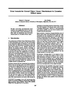
(a)

(b)

Please see Appendix A for the proof. Corollary 3. If each class has the same number of samples, ∀k, Nk = n, then (c) r C − 1 1 Figure 1. (a) — (c) Illustration of the Identity Sphere and Variation km0k k = , and cos θkl = − , ∀ k 6= l (8) Space. (a) When C = 3, it is a circle in 2D space and the Identity nC C −1 We can easily prove Corollary 3 by setting Nk = n in Theorem 2. Corollary 3 says that with equal samples in all classes, the C Identity Vectors distribute on a hypersphere q C−1 of radius rC = nC . Moreover, the angle between any two Identity Vectors is constant, and always larger than 90◦ . This means that the Identity Vectors are maximally spread out on the hypersphere. (They form the vertices of a regular simplex in RC−1 .) We may therefore call this the Identity Sphere. Figures 1(a) and 1(b) show the Identity Spheres for C = 3 and 4.

We now study the properties of Variation Space, the subspace spanned by V3 . We will prove that in this subspace, (a) all class means project to zero; and (b) the within-class variations of each class lie in orthogonal subspaces. eb Theorem 4. In WFLD, if V3 is the set of eigenvectors of S associated with λb = 0, then all class means project to 0: e k = 0. V3> m

(9)

e b v = 0. Proof. For any eigenvector v ∈ V3 , we have v> S e b = P> Sb P, so v> P> Sb Pv = 0. If we replace Sb But S with Equation (2), then 0

=

C X

N k v > P> m k m > k Pv

(10)

e k k2 Nk kv> m

(11)

k=1

=

C X

4.1. Geometric structure Let’s explore the geometric structure of Variation Space. Lemma 5. The inner product of any two whitened samples ei and x ej is: x

4. Variation Space

∀ k,

Vectors are vertices of an equilateral triangle; (b) When C = 4, it is a sphere in 3D space and the Identity Vectors are vertices of a regular tetrahedron; (c) An illustration of the geometric structure of Variation Space. Note that different shapes (colors) represent distinct classes. Class One has two samples lying on a vertical line, and both are orthogonal to Class Two, which has three samples evenly distributed on a circle.

k=1

This is a sum of squared norms, which is zero if and only if e k = 0. But this is true for each term is zero. Hence v> m e k = 0. any v ∈ V3 , and thus V3> m

e> ej x i x

 =

1− − N1

1 N

if if

i = j, i 6= j.

(12)

Please refer to Appendix B for a proof. Theorem 6. After projecting onto Variation Space, any two ej = x0j ∈ Ll , have ei = x0i ∈ Lk and V3> x vectors V3> x their inner product given by:  1  1 − Nk 0> 0 1 − xi xj =  Nk 0

if i = j and Lk = Ll , if i = 6 j and Lk = Ll , if i = 6 j and Lk = 6 Ll .

(13)

Again, we defer the proof to Appendix C so as not to distract from the main flow of our paper. Theorem 6 says that within Variation Space, any two classes lie in orthogonal subspaces. This can be seen from the last clause of Equation (13). Because of this, the within-class variation of each class do not overlap, but instead occupy distinct regions in the subspace Rrt −rb . Moreover, the Theorem also reveals how class samples are distributed in Variation Space, as shown in the next Corollary.

Corollary 7. After projecting onto Variation Space, all vectors from the same class Lk have the same length q 1 − N1k ; and any two vectors are separated by a constant angle θk , where cos θk =

−1 Nk −1 .

Here then is the whole picture of Variation Space. (1) Different classes share the same mean (Theorem 4); (2) Any two classes are orthogonal to each other (Theorem 6); (3) The Nk vectors for each class are equally distributed over a hypersphere of dimension Nk − 1 (Corollary 7). That is, the Nk vectors form a regular simplex. Figure 1(c) shows an example of Variation Space for two classes N1 = 2 and N2 = 3.

5. Practical Considerations 5.1. Existence conditions The Identity and Variation Spaces do not always exist; their existence depends on rb , rt , and rw respectively. For the Identity Space to exist at its maximum extent (size = C − 1), a sufficient condition is that (a) all data samples are linearly independent, and (b) D ≥ N − 1. This is also the sufficient condition for Variation Space to exist at its maximum size of N − C. Moreover, in this case, the size of Mixed Space is zero. This is the ideal situation because all class samples are neatly separated into Identity Space and Variation Space. Equation (4) now becomes: V = [ V1 | V3 ]. Note that V is an (N −1)×(N −1) orthogonal matrix, and thus invertible. In practice, Identity or Variation Space does not always exist because the sufficient condition (D ≥ N − 1 and linear independence) may not be satisfied. To encourage their existence, we implicitly transform the data into a highdimensional space by using the kernel trick [1]. There are two reasons to employ the kernel mapping function ϕ. First, the function ϕ can map two linearly dependent vectors xi and xj onto two linearly independent ones ϕ(xi ) and ϕ(xj ) [4]. Second, the mapped space {ϕ(xi )} could have arbitrarily large (even infinite) dimensionality [9]. After mapping the original space into the high-dimensional space with some function ϕ, we then maximize the Fisher Criterion in the new transformed space. This method is termed kernel WFLD (kWFLD) hereafter.

5.2. Decomposition and Representation ei ∈ Lk into We can thus decompose any training point x two components: ei x

ei + V3 V3> x ei = V1 V1> x > > e ei = V 1 V 1 mk + V 3 V 3 x = V1 m0k + V3 x0i .

(14) (15) (16)

ei is the projection onto Variation Space, where x0i = V3> x ei = V1> m e k is the projection onto Idenand m0k = V1> x tity Space. This decomposition follows because V1 V1> + ei ∈ Lk can be decomV3 V3> = I. Thus, any sample x posed into m0k (the identity component), and x0i (the variation component). Furthermore, x0i ∈ RN −C has a sparse representation (only Nk − 1 nonzeros) because the withinclass variation of each class is distinct (see Theorem 6). To recap, we have achieved a clean decomposition of a sample into its identity and variation components. This has the following merits. 1. It provides a way for efficient data representation. Any data point xi ∈ RD can be decomposed into its identity vector m0k ∈ RC−1 and its variation vector x0i encoded by Nk − 1 nonzero numbers, requiring only C + Nk − 2 numbers to represent it. Note that C and N could be  D, e.g. in face recognition, typically D ≈ 104 , while C ≈ 100 and Nk ≈ 10. 2. It combines the strengths of PCA (which is suited for representation, not classification) and the FLD (which is meant for classification, not representation). The identity vector m0k is best for classification according to the Fisher Criterion, while the vector x0i makes lossless reconstruction possible by retaining the variation information.

6. Experiments 6.1. Discriminability of Identity Space We perform face and digits recognition by using two datasets. The experimental setting is as follows. For PCA, we take the top C principal components, where C is the number of classes; for LDA, we apply PCA first by keeping 95% eigen-energy, followed by LDA; for kernel WFLD, we use Gaussian kernel. After projection, we use 1NN to perform classification. The recognition rate is reported by averaging over 20 runs. 1. Banca dataset [2] contains 52 subjects, and each subject has 120 face images, which are normalized to 51 × 55 in pixels. By using a web cam and an expensive camera, these subjects were recorded in three different scenarios over a period of three months. Each face image contains illumination, expression and pose variations because the subjects are required to talk during the recording (Fig. 2(a)). 2. MNIST dataset is derived from the NIST dataset, and has been created by Yann LeCun [8]. This dataset of handwritten digits (0 00 −0 90 ) has a set of 70, 000 examples in total. The digits have been centered and normalized to 28 × 28 in pixels. Fig. 2(b) shows a sample of MNIST digits images.

(a)

when Identity Space does not exist in the original data space when N > D, we can still create the most discriminant subspaces (aka Identity Space) by using the kernel method. Another strength of WFLD and kWFLD is efficiency. To classify an unknown point, WFLD or kWFLD needs to compare it with C Identity Vectors, whereas PCA and LDA require nC comparisons. For digits recognition, C = 10 and n = 600, so WFLD is 600 times more efficient in terms of storage and computation.

6.2. Discriminability of Variation Space

(b)

We now compare the discriminative power in Identity Space and Variation Space. We do this by taking a weighted sum of dVk and dIk : dk = αdIk + (1 − α)dVk ,

(c)

Figure 2. Samples of real data: (a) Banca faces; (b) MNIST digits; (c) PIE faces. For (a) and (c), each row represents one person. Note that PIE dataset only presents illumination variation; whereas, Banca dataset presents more variations, such as illumination, pose, and expression.

For face recognition, we randomly choose n training samples from each subject, n = 2, · · · , 12, and the remaining images are used for testing. For each set of n training samples, we employ cross validation so that we can compute the mean and standard deviation for classification accuracies. As shown in Table 1, we observe that for all methods, the more training samples, the greater the recognition accuracy. Kernel WFLD achieves around 2% better accuracy than WFLD. This shows that kernel method makes classes more separable in the high dimensional space. However, this performance difference is only slight, because Identity Space already exists in the original space for linearly independent samples with D ≥ N − 1. For digits recognition, we randomly choose n = 100, · · · , 600 training samples from each class, and the remaining images are used for testing. As shown in Table 2, WFLD produces the worst performance among all four methods. The reason is that Identity Space does not exist, so that identity and variation information are mixed together in Mixed Space. Kernel WFLD is always the best classifier in terms of the classification accuracy; it is also the most stable classifier in terms of having the smallest standard deviation. The gap between kWFLD and the second best is around 10%. All these results demonstrate that even

0 ≤ α ≤ 1.

(17)

where dIk is the distance from the query point to each Identity Vector and dVk is the distance from the query point to class Variation Space. The classification is performed by using the minimum distance: L? = arg minLk dk . Obviously, when α = 1, we are using only Identity Space, and when α = 0, we are using only Variation Space. To illustrate, we will use the Banca dataset for face recognition under varying illumination, pose, and expression. The experimental setting is thus: From the Banca dataset, we choose n = 2, 4, 6, 8, 10, 12 samples per class as the training set, and the rest for testing. We then vary α ∈ [0, 1] in steps of 0.1, and in each case classify the testing samples according to minimum distance. We repeat the sampling 20 times to compute the mean and standard deviation of classification accuracy. Figure 3 shows the results 1 . We observe that: 1. Variation Space does contain some discriminative information. This can be seen in the row where α = 0: the accuracies are significantly better than random 1 guessing (= 52 = 1.92%). 2. Identity Space is more discriminative than Variation Space, by comparing the accuracies for α = 0 and α = 1. More precisely, Identity Space achieves at least 33% greater accuracy than Variation Space. 3. Variation and Identity Spaces overlap a lot in terms of discriminability. This is suggested by the fact that when α = 1, the performance is approximately the best. This substantiates the effectiveness of Identity Space as a pattern recognition tool. 1 For the purpose of clear visualization, we only plot the mean rates without the standard deviation.

#. PCA LDA WFLD kWFLD

Table 1. BANCA: Classification accuracy (%) with different training set size. 2 4 6 8 10 12 38.30 (1.57) 54.45 (1.78) 65.37 (0.74) 73.63 (1.04) 78.54 (1.33) 82.34 (1.31) 65.33 (3.71) 79.81 (2.19) 90.15 (0.94) 94.20 (0.85) 95.93 (0.79) 96.92 (0.48) 70.45 (1.74) 85.33 (1.67) 90.87 (0.77) 93.85 (0.56) 94.35 (0.60) 95.12 (0.35) 70.26 (1.74) 86.89 (2.12) 92.29 (1.21) 95.44 (0.59) 96.47 (0.56) 97.04 (0.41)

#. PCA LDA WFLD kWFLD

Table 2. MNIST: Classification accuracy (%) with different training set size. 100 200 300 400 500 600 82.76 (0.57) 85.23 (0.50) 86.49 (0.34) 87.13 (0.27) 87.75 (0.21) 88.14 (0.24) 82.69 (0.53) 85.12 (0.37) 86.10 (0.29) 86.72 (0.23) 87.24 (0.21) 87.50 (0.23) 63.38 (1.03) 76.41 (0.49) 79.72 (0.34) 81.37 (0.29) 82.26 (0.27) 82.84 (0.25) 92.79 (0.24) 94.84 (0.12) 95.70 (0.11) 96.19 (0.11) 96.54 (0.08) 96.79 (0.08)

1

0.9

0.8

Accuracy

0.7

0.6

n = 02 n = 04 n = 06 n = 08 n = 10 n = 12

0.5

0.4

0.3

0.2

0

0.1

0.2

0.3

0.4

0.5

α

0.6

0.7

0.8

0.9

1

Figure 3. Face recognition by using both Identity and Variation Spaces with varying training set size n = 2, ..., 12. When α = 1, we are using only Identity Space; when α = 0, we are using only Variation Space. It shows that Identity Space contains much more discriminant information than Variation Space.

controls the illumination. Because the WFLD is a lossless invertible transform, when c = 1 we get back exactly the input image. Here, it is clear from the shadows that the light source is from the left of the face. When c = 0, the illumination appears frontal and there is no shadow. This is because in the PIE dataset, the illumination varies approximately symmetrically from left to right, so that the mean face is frontally illuminated. Since c = 0, we are effectively reconstructing the face using only its identity component and suppressing its variation component. This appears to have suppressed shadows as well. When c = −1, we observe that the illumination has moved to the right; while for c = 2, 3, the illumination has become harsh. Actually, we have a whole subspace (the class variation ei ) to vary the illumination. Any vecspace of the sample x tor in this subspace will synthesize a new illumination. We have merely shown the trivial case of varying the magnitude of the projected sample.

6.3. Face Synthesis Our next experiment attempts to synthesize face images under varying illumination. We know from Section 5.2 that we can use WFLD to cleanly decompose any sample into its identity and variation components, modify each component separately, and then reconstruct a new sample. More ei , we synthesize a new specifically, given a face image x b(c) = V1 V1> x ei + cV3 V3> x ei , where c is a image using x parameter for us to control the amount of variation. To illustrate, we will use the CMU PIE [10] dataset for illumination synthesis. We choose C = 68 subjects, each having 24 frontal face images taken under a wide range of lighting conditions. All face images are aligned based on eye coordinates, and cropped to the size of 70 × 80(= D) pixels. Figure 2(c) shows some PIE face images. Figure 4 shows two examples of illumination synthesis as we vary c = −1, . . . , 3. It is evident that this parameter

Figure 4. Two examples of illumination synthesis, as c, the usercontrolled parameter is varied. The original input images are in column c = 1, because the WFLD is an invertible transform.

Our final experiment shows that WFLD may be used to swap face illuminations. Fig. 5 shows two examples of the variation synthesis. Given two novel face images under different lighting, we synthesize the face images with the swapped variation components. In this case, the variation components represent the face illumination. To evaluate the

synthesis quality, we also show the real face images under the swapped lighting. Our synthesized face images are comparable to the real face images, except the shadows. The reason is the shadows are generally encoded as high-order information. However, our theory is based on second-order information (scatter matrices).

(a)

optimal subspace for pattern classification in terms of the Fisher Criterion, and then mathematically proved its property: all samples from one class project onto its Identity Vector, which is also its class mean. Variation Space was defined as the least discriminant subspace for pattern classification, and it contains no class means to be used for classification. We further showed their geometric structures, the conditions required for them to exist. When the conditions are not satisfied, the kernel trick was proposed to encourage the existence. To assess the performance of these two spaces, we ran face and digits recognition by using the Identity Space, and synthesized face images by using the Variation Space. The results show the power of WFLD as a pattern classification tool and as a data decomposition tool. One limitation of our work is generalization. The property of clean class separation that we prove applies only to the training data, and not necessarily to novel, unseen data. Pre-whitening the FLD does not guarantee improved generalization, so standard regularization techniques [6] can still be applied here. However, it is clear from the linearity of our proofs that if novel data lie within the subspace of the training data, then they will also be perfectly separated. Thus, the crux is whether training data is representative of novel data — a problem common to all machine learning methods, not just to the FLD.

A. Proof of Theorem 2 e b = VΛb V> . Within IdenProof. The whitened Sb is decomposed as S tity Space, λb = 1. That is: Λb = I corresponding to the set of eigenvece b V1 = I. Because S e b = P> Sb P, it is easy to see tors V1 . Thus, V1> S that V1> P> Sb PV1 = I. If we replace Sb with Equation (2), I

(b)

Figure 5. Two examples of variation synthesis. For (a) and (b), the leftmost column is the given face images with different identities and variations (lighting); the medium column shows the synthesized face images with the swapped lighting; the rightmost column shows the real face images with the swapped lighting.

=

V1> P> Sb PV1 =

C X

Nk V1> P> mk m> k PV1

=

C X

Nk m0k m0> k

(19)

k=1

√ √ Now let’s denote M = [ N1 m01 , · · · , NC m0C ] ∈ R(C−1)×C , then we can rewrite Equation (19) as MM> = IC−1 .

7. Conclusion We have proven a number of important theoretical properties of the WFLD. As such, we argue that the WFLD is the correct way to compute the FLD. In so far as the original objective of the FLD was to eliminate within-class variation and maximize between-class variation, the pre-whitening step guarantees this objective. Note that we are not claiming that the WFLD is better than the Bayes’ Classifier. Instead, we are merely explaining that elegant properties emerge when the FLD is computed correctly. More precisely, the WFLD decomposes pattern vectors into two neat subspaces with useful properties: Identity and Variation Spaces. We defined Identity Space as the

(18)

k=1

(20)

where IC−1 is the × (C − 1) identity matrix. Since the total P(C − 1) mean is zero, i.e. Nk m0k = 0, it is easy to see that Mi = 0 (21) √ √ where i = [ N1 , · · · , NC ]> . Equations (20) and (21) shows that the rank of M is C − 1 and its only nullspace is i ∈"RC . # M > To compute M M, we first define Q = ∈ RC×C . √1 i> N

Thus, " QQ> =

M √1 i> N

#

h

M>

√1 N

i

i

= IC

(22)

P Here N = i> i = Nk . Since Q is a full rank, square matrix, Equation (22) shows that Q is an orthogonal matrix, i.e. QQ> = Q> Q = I. Hence, 1 (23) Q> Q = M> M + ii> = I N

And thus, M> M = I −

1 > ii N

(24)

On the other hand, i hp i hp 0 > Nk Nl m0> Nk Nl . M> M = k ml , ii =

0 x0> i xj

B. Proof of Lemma 5 (30)

e = [e eX e > = I. Because of eN ], then X We further define X x1 , · · · , x e e the zero global mean, X1 = 0. Thus, rank(X) = N − 1 and its only nullspace is 1 ∈ RN . Using the same trick as in Equations (22) to (24), we get e = I − 1 11> e >X X (31) N e >X e are 1 − 1 , and off-diagonal ones are − 1 . The diagonal entries of X N N This completes the proof.

C. Proof of Theorem 6 Proof. 0 x0> i xj

“ ”> “ ” ei ej V3> x V3> x

=

(32) (33)

=

“ ” > e> ej = x e> ej x I − V1 V1> x i i V3 V3 x “ ”> “ ” e> ej − V1> x ei ej x V1> x i x “ ”> e> ej − V1> m ek el x V1> m i x

=

e> ej x i x

(36)

= =

−

0 m0> k ml

V1 V1>

(34) (35)

V3 V3>

Remarks: (1) Equation (33) is derived from + = I. (2) Equation (36) is derived from Theorem 1. It remains to consider three cases, with the help of Equation (27) and Lemma 5: 1. When i = j, immediately Lk = Ll , then 0 x0> i xj

= =

0 e> ej − m0> x i x k ml „ « „ « 1 1 1 1− − − N Nk N

(37) 1 =1− (38) Nk

2. When i 6= j and Lk = Ll , then 0 x0> i xj

= =

0 e> ej − m0> x i x k ml „ « 1 1 1 − − − N Nk N

(39) 1 =− Nk

(40)

= =

(25)

Considering Equations. (24) and (25), we see that 8 √ Nk Nl < p 1− if k = l; 0> 0 √ N Nk Nl mk ml = (26) : − Nk Nl if k 6= l. N ( 1 1 −N if k = l; 0 Nk That is: m0> m = (27) k l 1 if k 6= l. −N s 1 1 (28) − . When k = l, km0k k = Nk N √ 0 m0> − Nk Nl k ml √ √ = When k 6= l, cos θkl = km0k kkm0l k N − Nk N − Nl (29) This completes the proof.

Proof. After pre-whitening, P> St P = I. That is: X X ei x e> I = P> xi x> x i P= i

3. When i 6= j and Lk 6= Ll , then 0 ej − m0> e> x i x k ml „ « 1 1 − − − N N

(41) =0

(42)

This completes the proof.

References [1] M. Aizerman, E. Braverman, and L. Rozonoer. Theoretical Foundations of the Potential Function Method in Pattern Recognition Learning. Automation and Remote Control, 25:821–837, 1964. [2] E. Bailly-Bailli´ere, S. Bengio, F. Bimbot, M. Hamouz, J. Kittler, J. Mari´ethoz, J. Matas, K. Messer, V. Popovici, F. Por´ee, B. Ru´ız, and J. P. Thiran. The BANCA Database and Evaluation Protocol. In The 4th International Conference on Audio- and Video-based Biometric Person Authentication, pages 625–638, 2003. [3] P. Belhumeur, J. Hespanha, and D. Kriegman. Eigenfaces vs. Fisherfaces: Recognition Using Class Specific Linear Projection. IEEE Transactions on Pattern Analysis and Machine Intelligence, 19(7), 1997. [4] C. J. C. Burges. A tutorial on support vector machines for pattern recognition. Data Mining and Knowledge Discovery, 2:121–167, 1998. [5] R. Duda, P. Hart, and D. Stork. Pattern Classification, 2nd Edition. John Wiley and Sons, 2000. [6] J. Friedman. Regularized Discriminant Analysis. Journal of the American Statistical Association, 84:165–175, 1989. [7] K. Fukunaga. Introduction to Statistical Pattern Recognition, 2nd Edition. Academic Press, 1990. [8] Y. LeCun, L. Bottou, Y. Benjio, and P. Haffner. GradientBased Learning Applied to Document Recognition. Proceedings of the IEEE, 86(11):2278–2324, November 1998. [9] B. Sch¨olkopf and A. J. Smola. Learning with Kernels: Support Vector Machines, Regularization, Optimization, and Beyond. The MIT Press; 1st Edition, 2001. [10] T. Sim, S. Baker, and M. Bsat. The CMU Pose, Illumination, and Expression Database. IEEE Transactions on Pattern Analysis and Machine Intelligence, 25(12):1615 – 1618, December 2003. [11] T. Sim, S. Zhang, J. Li, and Y. Chen. Simultaneous and Orthogonal Decomposition of Data using Multimodal Discriminant Analysis. In IEEE International Conference on Computer Vision, 2009. [12] H. Yu and H. Yang. A Direct LDA Algorithm for HighDimensional Data - with Application to Face Recognition. Pattern Recognition, 34(10):2067–2070, 2001. [13] S. Zhang and T. Sim. When Fisher Meets Fukunaga-Koontz: A New Look at Linear Discriminants. In IEEE Conference on Computer Vision and Pattern Recognition, pages 323– 329, June 2006. [14] S. Zhang and T. Sim. Discriminant Subspace Analysis: A Fukunaga-Koontz Approach. IEEE Transactions on Pattern Analysis and Machine Intelligence, pages 1732–1745, October 2007.