IEEE ROBIO 2007 Paper - CiteSeerX

Proceedings of the 2007 IEEE International Conference on Robotics and Biomimetics December 15 -18, 2007, Sanya, China

Action Classification of 3D Human Models Using Dynamic ANNs for Mobile Robot Surveillance Theodoros Theodoridis and Huosheng Hu Department of Computer Science, University of Essex Wivenhoe Park, Colchester CO4 3SQ, U.K. {ttheod, hhu}@essex.ac.uk

Abstract— This paper presents an alternative approach on physical human action classification implemented by mobile robots. In contrast with other action recognition methods, this research indicates the best configuration topology of a number of dynamic neural networks to be used in 3D time series classification by showing several comparison performances. In this action recognition investigation we demonstrate high level network granularity on dynamic classification and class discrimination of normal and aggressive action recognition. An interconnection between an ubiquitous 3D sensory tracker system and a mobile robot is set to create a perception to action architecture capable to perceive, process, and classify physical human actions. The robot is used as a process-to-action unit to process the 3D data taken by the tracker and to eventually generate surveillance assessment reports pointing towards action-class matchings as well as generating evaluation statistics which signify the quality of the actions recognized. Index Terms— Ubiquitous robotics, dynamic NN classifiers, kinematic models, time domain feature extraction.

I. I NTRODUCTION Human action analysis, in terms of recognizing and classifying different physical activity patterns has been a challenging task in 2D and 3D computer vision. In previous frameworks researchers addressed the 3D action classification problem using various methods. Multiple calibrated cameras have been used by [1][2] for a view-independent approach to the classification of human gestures through data fusion and feature extraction using motion history and energy volumes. In [1], a Bayesian classifier processes 3D invariant statistical moments as feature vectors whereas [2] focuses on an efficient Fourier transformation performed on the vertical axis of a cylindrical coordinate system used to robustly extract visual motion descriptors which are classified by distance-based methods. A modified version of the matching pursuit algorithm proposed by [3], was used for decomposing arbitrarily input postures into linear combinations of primary and secondary elementary postures called atoms. A Hidden Markov Model (HMM) and atom decomposition techniques have been used for the gesture recognition part where each gesture is decomposed in a number of atoms while their temporal evolution is recognized by the HMM. Similar to our work, [4] has used a dynamic programming algorithm to process 3D joint features so that to segment and recognize actions by improving the overall accuracy with a Multi-Class AdaBoost algorithm. In [5], a 3D approach that

978-1-4244-1758-2/08/$25.00 © 2008 IEEE.

371

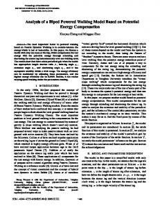
builds 3D model-based invariants, analyzes perceived actions as unique curves in a 3D invariance-space surrounded by an acceptance volume. The curves have unique distances, calculated by invariant Euclidean space representations, which is what the action models of this approach handle so that to generate action classification matchings. Opposite to [1][2], in [6] uncalibrated moving cameras were used along with a dynamic epipolar geometry method to capture readings from 3D points and thereafter to generate 4D trajectories in space and time. In our work, a number of dynamic neural networks from Matlab’s NN toolbox [7], have been used to compare which network performs better regarding the classification accuracy as well as the discrimination capability to distinguish between normal and aggressive actions through an off-line processing. Fig. 1 illustrates the hardware configuration setting of the system architecture used. More analytically, a person is shown to act in a 3D environment performing some physical activity. At the same time two external devices, the 3D tracker (Vicon system) and a mobile robot (SCITOS G5), cooperate as a perception to action unit to produce surveillance assessment reports indicating analytical action classification. The rest of the paper is organized as follows: In section II, the system’s software architecture is introduced where a number of modules are explained analytically. Section III presents a number of experiments showing the best action classification performances. Finally, section IV points out some conclusions and future work derived from the current architecture used.

Fig. 1. Configuration setting showing an actor’s action performance in a 3D environment, captured by VICON and processed by a mobile robot.

II. S OFTWARE A RCHITECTURE A. Vicon Modules The Vicon system encloses three main modules depicted by Fig. 2. The Image Acquisition module is a low level unit used for capturing and fusing data taken from nine high resolution infrared cameras. The Kinematic Model Extraction module is a commercial software where 3D models are designed according to the alignment of the markers on an object/body. Such kinematic models emphasize mainly on the limbs and more specifically on the end effectors since the end points of the limbs are the ones which act to produce physical actions. The last, Data Sampling module, configures the sampling frequency of the image capturing per second to finally generate time series. Since we deal with aggressive physical actions it is rational to set up high frequency so that to avoid loss of information produced by high speed aggressive actions. B. Robot Modules These modules constitute the core of the software architecture design. From the image processing to the time series generation, Vicon prepares a set of activity information expressed in time series so that to send it to the robot for classification processing and evaluation assessment (see Fig. 2). Eight modules act together to preprocess the activity data, categorize the data in classes, and simulate part of the data to show the action classification performance. 1) Data Processing: The first module, Data Re-Sampling, is used to scale the sampling rate of the data into lower or higher frequencies by increasing the sampling time from 5ms to 1sec. The initial sampling time of the data has been set to 200Hz where each frame is captured every 5ms so that analytical trajectories to be generated. The second module, Z-C Filtering, is used to filter zerocrossing reading ambiguities which can occur from a number of parameters such as temperature, vibration, or high frequency. When data values cannot be read properly, Vicon grounds these readings to zero. To eliminate this phenomenon we simply search for zero value readings and replace them with previous non-zero ones (1).  xi = xi+1 , if i = 1 if xi = 0 (1) xi = xi−1 , otherwise The third module, G/L Transformation, is a global-tolocal transformation method used to provide independency of body sizes and gender by isolating ambiguous variations of actions performed by human subjects acting in different locations and under different orientations. A local frame of reference, generated from Vicon’s global one, is regarded as a secondary coordinate system coming from the actor’s front body. Fig. 3(a) shows this reference point coming from the central shoulder marker B located at the back neck. A cylindrical coordinate system has been used so that all the performed actions to come and rotate around the actor’s spinal column. The cylindrical coordinates are inspired by

372

Fig. 2. Software architecture showing the collaboration of the Vicon system and a mobile robot to generate surveillance assessment reports.

a Cartesian global setting (Gcrt) with the only common axis being the z ∈ [0, ∞) denoting the actor’s height from which rotation takes place. The vectors r = x2 + y 2 ∈ [0, ∞) indicate extensions of lines, right to the z axis, coming from the reference point B to any of the end effector markers ⊕. The angle θ = arctan(x/y) ∈ (−π, +π] shows the orientation of the cylinder around the z axis. The arc tangent of the angle θLcld (2), is taken from the middle point of the right and the left marker (A, C) which is the plane where the actions express as indicated by the vector rLcld , Fig. 3(a). θLcld = atan2((Ax + Cx )/2, (Ay + Cy )/2)

(2)

The vectors r coming from the shoulder model to every individual end effector marker ⊕, are normalized by transforming them to unit vectors so that to have bounded magnitude without affecting their directions. This is achieved by computing the Euclidean distance dr of every vector r (3), the overall distance D among the vectors, estimated by (4), and finally their values are divided by the distance D as it is shown by the equation groups (5) and (6), to produce unity extensions.  dir = (rxi − Bx )2 + (ryi − By )2 (3)   4  D =  (dir )2

(4)

i=1 i are the extension vectors of the marker i, i = where rxy {1, 2, 3, 4} ≡ {rwrs, lwrs, rank, lank}. All the vectors r

(a)

(b)

Fig. 3. (a) Global and local (G/Lcld) cylindrical coordinate system for the rotation, and (b) extension vectors r for the translation transformation.

are normalized in the interval {0, 1} and correctly translated in space. A very important fact is that the unit vector transformation converts all the vector values to a positive plane. Due to the positive sign conversion the vector directions change when initial negative values presented. To prevent this occurrence we separate the right and left limbs in a positive and a negative plane respectively. With this separation all the actions coming from the left or the right limbs have reference intervals {0, +1} for the right limbs, and {0, −1} for the left limbs in x and y plane. In equation group (5), the rxi r vectors perform unit normalization, translation, and sign conversion for the right hand side whereas in (6) the vectors ryi l perform unit normalization and sign conversion for the left hand side.

rxi r

1 − (1 − 2| = 2

i rx r D

|)

, ryi r = −|

ryi r ri |, rzi r = zr D D

(5)

ryi rxi l ri |, ryi l = | l |, rzi l = zl (6) D D D To finalize the G/L transformation procedure, a rotation matrix around the z axis is employed to rotate the four normalized vectors to the front plane of the body (7). rxi l = |

⎡ i ⎤ ⎡ i ⎤ rxlr cosθLcld −sinθLcld 0 rxlr Rz (θLcld ) = ⎣ryi lr ⎦ = sinθLcld cosθLcld 0 ⎣ryi lr ⎦ (7) rzi lr 0 0 1 rzi lr The fourth module is the Feature Extraction module. Time domain features extracted by this module regard spatially interpolated points of the performed activities in space. On the other hand, activity features which relate limb velocities, joint angles, or extensions, as discussed by [4], are not our main concern in this work. A 13th -dimensional feature action vector constitutes the networks’ input space:  = [rwrsTxyz lwrsTxyz rankTxyz lankTxyz ΘT ]T , where the A l ankle and the wrist vectors (ank, wrs) have 3-dimensions plus the orientation θ vector. Similar to [4], each feature action vector generates a combination of motions related to multiple concatenated 3D points or trajectories. The dynamics of the overall feature action vector performance is learnt by a dynamic neural network to produce matching classes. According to the 13th -dimensional feature vector, the input space of the network will also be 13th -dimensional whereas the networks’ output remained one for serial class generation. The fifth module, Normalization, rescales the data within the interval {−1, 1} for greater network classification efficiency by dividing all the data matrices with 1000. 2) Classification: Dynamic nonlinear ANN classifiers have been chosen to solve the physical action recognition problem. The spreadability of the normal action clusters can be discriminative separable in space while the spreadability of the aggressive action clusters not only overlapping each other by neighbouring aggressive action clusters, but are also mixed with even near normal action clusters. As mentioned in [4], the high dimensionality of 3D joint positions in space creates

373

computational complexity by making the important features of the actions less visible for the classifier and the observed measurements may have significant spatial and temporal variations. Therefore, the purpose of dynamic networks used is to process and discriminate sequences of actions, spread in a nonlinear 3D space, so that to generate distinct models for each individual action through training examples based on the dynamic evolution of poses. Since neural networks are problem depended algorithms it is difficult to know beforehand how large a network should be for a specific application [7], hence, heuristic methodology is what should be applied to determine an appropriate network. One of the main concerns of this study is to compare the classification performance of several dynamic networks with different structure. The sixth module Dynamic Networks, emphasizes on the most significant characteristics of dynamic networks, training algorithms, and error functions as well as their abilities to handle time series because of the memory they have from which they can be trained to learn time-varying patterns. • Dynamic Networks The comparison analysis that is carried out in later chapters, evaluates three types of networks: i. FTDNN, this is a feedforward dynamic network with a tapped delay line (TDL) at the input layer which is what denotes its dynamics to handle time continuities which improves its speeding ability since it does not have to perform dynamic backpropagation for the gradient computation. ii. LRNN, this is an Elman type network with a recurrent feedback delay loop appeared to every hidden layer denoting a short-term memory [8][9]. iii. DTDNN, this network (similar to FTDNN) has a number of TDLs allocated to the inputs of every layer. • Training Functions Thirteen training function have been tested whereas among them, three of the most powerful ones presented distinctive results which have been used to train the networks. i. Levenberg-Marquardt, (trainlm function) is an optimization algorithm outperforming simple gradient descent and other conjugate gradient methods using the nonlinear least squares minimization [7][10]. ii. Quasi-Newton, (trainbfg function) is a line search algorithm which does not need to compute the Hessian matrix. This method is efficient for small structured network [7][11]. iii. Automated Regularization, (trainbr function) sets the weights and biases of the network randomly with specified distributions using statistical techniques to prevent data from overfitting [7]. • Error Functions Three error functions have been used to test the networks’ learning performance. The functions are: the mean squared error (mse function), the mean absolute error (mae function), and the mean squared error with regularization performance (msereg function). 3) Simulation: The seventh module, Simulated Class Outputs, simulates the already trained network to test the generalization performance of each individual network which outputs time series-based classes. A threshold filter is used to convert these resultant time series into unique matching numbers for easier manipulation. Hence, this method averages each class separately (8) and then compares the mean value with a fixed threshold to output a rounded number (9).

T T classj

Fclassj

N 1  = xi N i=1

⎧ ⎨ 1, if T classj ≥ [tj − (tj · γ)] and = T classj ≤ [tj + (tj · γ)] ⎩ 0, otherwise

(8)

(9)

T

where T classj represents the mean value of a particular time series which belongs to a class j, N is the overall number of the sampled data of a T classj , xi denotes each individual sample, Fclassj is the thresholded output class, tj is the target class number of a class j, and γ is a threshold used to create an interval where every current class is compared within it. Note that in (9), Fclassj is only used to improve the class recognition to be used for real applications such as the surveillance assessment reports and not for the performance comparison analysis. The final eight module, Class Evaluation, presents two evaluation methods to show the networks’ generalization performance. The first method, the standard deviation of the mean filtered class values (10), is used to show how the classified physical actions deviate from the mean; the less the deviation the better classification achieved.   N 1  σ= (xi − T classj )2 (10) N i=1 The second method is an analytical percentage evaluation process, a mean-based classification accuracy method (11), which computes how well the network can generalize by T comparing the T classj value of a simulated action class j, with the actual target class tj .

Pclassj =

⎧ ⎨ ⎩

|T classj | tj tj |T classj |

· 100%, if T classj ≤ tj · 100%, if T classj > tj

(11)

The seventh, Simulated Class Outputs and the eight, Class Evaluation module unify the Assessment Reports which outcome a detailed set of information stating the type of the actions (1-9) recognized, the behaviour of each individual action (normal(N) or aggressive(A)), and the estimated validity which yields a percentage evaluation (11) by computing the average performance of the simulated classes P classj .

and punching actions relevant equipment has been used such as punching pads and standing bags. The networks’ testing comparison performance has been divided in two parts. On the first, all the three networks are tested with a number of certain topological structures and learning parameters so that to determine which performs better. On the second part, the previously dominant best performance network, is tested given different training and error functions by keeping its internal structure unchanged. Regarding the input and output setting, thirteen inputs have been used to pass the whole 13th dimensional feature vector for processing. The hidden layers have been set in an decremental fashion beginning with high to low number of neurons from the first hidden to the last output layer. Finally, a single output has been used to yield serially the classified action targets. A. Dynamic Network comparison The purpose of this testing is to select the best network configuration among three and then to compare their performances. The networks’ structure, regarding the neuron/layer size, has been divided in six experiments where the three first experiments used one layer and three different neuron configurations, 3 , 6 , and 12 neurons. For the second experiments, two layers of 6 3 and 12 6 neurons have been used, while for the last experiment three layers were used of 6 4 2 neurons as it is shown on Fig. 5 and Fig. 6. Note that early experiments have also tried to solve this particular classification problem using more layers (≤5) as well as more neurons (≤48) but the results showed that the networks’ generalization suffered from overfitting. For this series of experiments, the training algorithm used was the LevenbergMarquardt (trainlm) since this method is considered as one of the fastest optimization gradient descent algorithms. The error function used was the conventional mean squared error performance function (mse). At this point all the networks have shown one distinct performance which can select the best configuration in neurons and layers. Table I summarizes the learning performances of the Fig. 5 and Fig. 6. TABLE I T RAINING (E) AND S IMULATION ((σ 2 ), (%)) P ERFORMANCE S UMMARY. NN DTDNN

III. E XPERIMENTAL R ESULTS The types of actions have been taken from the every day life; such actions are: standing, waving, punching, kicking, etc [1][2][4]. Fig. 4 depicts an instance of each of the nine actions used in this analysis represented by a human kinematic model which is decomposed in six segmented models (head, left and right limbs). To make the expression of the actions more realistic, a human partner has been used to help the actor’s performance for the handshaking, pushing, and pulling actions, whilst for the slapping, kicking,

374

FTDNN

LRNN

N/L

E(mse)

SD (σ 2 )

P classj (%)

3 6 12 6 3∗ 12 6 6 4 2 3 6 12 6 3∗ 12 6 6 4 2 3 6 12 6 3 12 6 6 4 2∗

7.72e-03 1.48e-04 2.97e-05 3.09e-08 4.19e-08 2.54e-04 2.75e-03 1.69e-05 4.22e-07 1.03e-07 1.21e-08 7.32e-07 5.63e-03 5.87e+00 6.61e-06 4.92e-03 2.97e-05 1.11e-06

0.1239 0.0853 0.0920 0.0148∗ 0.0641 0.0933 0.1233 0.0886 0.1054 0.0160∗ 0.0963 0.0906 0.1704 0.0961 0.1704 0.3730 0.0920 0.0327∗

96.43 97.76 96.12 99.40∗ 97.72 95.93 96.66 98.81 98.05 99.18∗ 96.91 97.43 94.07 97.73 97.14 87.53 96.12 99.06∗

∗best simulation performances under certain neuron/layer (N/L) structures

(a)

(b)

(c)

(d)

(e)

(f)

(g)

(h)

(i)

Fig. 4. Instant action representation of the nine physical actions expressed by 3D kinematic human models. Normal actions: (a) Standing, (b) Handshaking, (c) Waving, (d) Clapping. Aggressive actions: (e) Pushing, (f) Pulling, (g) Slapping, (h) Kicking, (i) Punching.

(a)

(b)

(c)

Fig. 5. Training performance comparison testing six different structures of all the three networks individually. The square-marked performances show one of the selected minimum errors achieved in relation with the corresponded neuron/layer structure used. TABLE II

TABLE III

T RAINING AND S IMULATION P ERFORMANCE C OMPARISON OF THE

S URVEILLANCE A SSESSMENT R EPORT T HROUGH S IMULATION .

T RAINING AND E RROR F UNCTIONS . Train F trainlm trainbfg trainbr traincgb traincgf traincgp traingd traingda traingdm traingdx trainoss trainrp trainscg Error F mse mae msereg

Train E(mse) 3.09e-08 1.05e-03 2.69e-03 2.28e-03 7.90e-03 9.87e-03 1.85e-01 1.09e-01 1.55e-01 7.75e-02 7.64e-03 8.94e-03 6.83e-03 Train E 3.09e-08 1.01e-02 9.04e-02

Action (Type) Standing Handshaking Waving Clapping Pushing Slapping Kicking Punching

P classj (%) 99.40 98.68 98.89 92.15 96.82 95.76 77.58 83.98 78.24 86.90 94.30 90.29 93.07 P classj (%) 99.40 98.72 87.61

Behaviour (N/A∗ ) N N N N A A A A

Validity (%) 99.99 99.98 99.96 100.0 99.13 100.0 100.0 100.0

∗where N : normal and A: aggressive actions

According to Table I, the DTDNN and the FDTNN networks have shown the most significant performances indicated at the 6 3 structure configuration with minimum learning errors of 3.09e − 08 and 1.03e − 07 respectively. In Fig. 5(a) and 5(b), the best learning performances, regarding the learning error, are shown by the dashdoted lines (structures: 12 6 ). However, the reason that the 6 3 structure is selected (squared lines) and not the 12 6 is because the simulation performance of the action recognition which uses a 40% of newly presented data, is what it strongly determines the best network structure. This is shown by Fig. 6(a) and 6(b) indicating the lower standard deviations of the simulated classes. The probability of sellecting a network structure from its simulation performance is a lot higher than sellecting

375

a structure from the training error performance. Both, the training error and the simulation performance show how well the networks can classify physical actions but only the simulation can show generalization results of newly comming data. In that sense, the neuron/layer structures have been selected according to the best-lower standard deviation and the percentage evaluations (11) of the simulated classes (Fig. 6) as well as from the second best learning error performance (Fig. 5). Observing Table I, it is clear that the network which has achieved the best simulation performance is the DTDNN, second came the FTDNN, and third the LRNN. B. Training and Error Function Comparison In overall, thirteen training and three error functions have been tested on the network which performed best (DTDNN) among the three standard structure configurations as the first testing has shown. The rest of the network’s configuration remained the same as in the previous experiment. Fig. 7 shows graphically and Table II analytically the learning and simulation performances of the thirteen training functions and the three error functions. The majority of the training and error functions used, led the network to inefficient generalization

(a)

(b)

(c)

Fig. 6. Simulation performance comparison, testing six different structures of all the three networks individually. The bars represent the standard deviations (SD) of the nine classes (0-8). The darker to the lighter bars show the lower (black) to the higher (white) SD of the simulated classes achieved from the mean.

(a) Fig. 7.

(b)

(c)

(d)

Training and error functions comparison. (a) and (c): training function testing, (b) and (d): error function testing.

results while the training error reached hardly the 1e − 03. Among these thirteen training functions, only three achieved good classification results; these functions are the trainlm function, the trainbfg function, and the trainbr function. Regarding the three error functions, the mean square error mse function has shown the best learning results. Eventually, the trainlm and the mse functions led the network to achieve the best training and simulation performances among the three others. IV. C ONCLUSIONS AND F UTURE W ORK This paper presented a dynamic NN action classification method by a mobile robot using a 3D ubiquitous sensory tracker. It has been shown analytically how the ubiquitous 3D tracker provides 3D motion data points generated by kinematic models when physical activities are expressed. The experimental work of this research demonstrated one of the most appropriate dynamic NN configurations by implementing several testing comparisons in terms of network types and structures, and different training and error functions. The outcome of this comparison proposes a final network type and configuration topology which can achieve 99.4% of physical action recognition performance capable to discriminate among nine actions and their corresponding behaviours as is shown in Table III. The dynamic network configuration derived is: nn→DTDNN, N/L→6 3 , trainF→trainlm, errF→mse, hiddenTF→tansig, outputTF→purelin, learningRate→0.01, samplingFreq→200Hz, epocs→1000, goal→1e − 20, init Weights→random, trainData→60%, testData→40%. Our next analysis will be focused on frequency domain

376

feature recognition so that to be independed from indoor ubiquitous environments and marker-depended techniques. R EFERENCES [1] Ferrer C.C., Casas J.R., and Pards M. Human model and motion based 3d action recognition in multiple view scenarios. In 14th European Signal Processing Conference, Universita di Pisa, 2006. [2] Weinland D.l., Ronfard R., and Boyer E. Motion history volumes for free viewpoint action recognition. In IEEE International Workshop on modeling People and Human Interaction (PHI’05), pages 1, 3, 5, 2005. [3] Chu C.W. and Cohen I. Posture and gesture recognition using 3d body shapes decomposition. In Proceedings of the 2005 IEEE Computer Society Conference on Computer Vision and Pattern Recognition (CVPR’05), volume 3, 20-26 June 2005. [4] Lv F. and Nevatia R. Recognition and segmentation of 3-d human action using hmm and multi-class adaboost. In 9th European Conf. on Computer Vision (ECCV’06), volume 4, pages 359–361, 2006. [5] Parameswaran V. and Chellappa R. View invariants for human action recognition. In 2003 IEEE Computer Society Conference on Computer Vision and Pattern Recognition (CVPR ’03), volume 2, pages 1, 3, 6, 2003. [6] Yilmaz A. and Shah M. Recognizing human actions in videos acquired by uncalibrated moving cameras. In Proceedings of the Tenth IEEE International Conference on Computer Vision (ICCV’05), volume 1, pages 150–157, 17-21 Oct. 2005. [7] Demuth H., Beale M., and Hagan M. Neural network toolbox users guide. Technical report, The MathWorks, 2006. [8] Husken M. and Stagge P. Recurrent neural networks for time series classification. Neurocomputing, 50(C):1, 2003. [9] Boden M. A guide to recurrent neural networks and backpropagation. Technical report, In The DALLAS project, Report from the NUTEKSupported Project AIS-8: Application of Data Analysis with Learning Systems, Sweden, 2002. [10] Lourakis M. and Argyros A. The design and implementation of a generic sparse bundle adjustment software package based on the levenberg-marquardt algorithm. Technical report, Institute of Computer Science, Heraklion, 2004. [11] Davidon W.C. Variable metric method for minimization. SIAM Journal on Optimization, SIOPT 1:1–17, 1991.