ifs documentation - ECMWF

IFS Documentation Cycle CY25r1

IFS DOCUMENTATION Part VII

ECMWF WAVE MODEL (CY25R1) (Operational implementation 9 April 2002)

Peter Janssen and Jean-Raymond Bidlot

Table of contents Chapter 1. Introduction Chapter 2. The kinematic part of the energy balance equation Chapter 3. Parametrization of source terms and the energy balance in a growing wind sea Chapter 4. An optimal interpolation scheme for assimilating altimeter data into the WAM model Chapter 5 Numerical scheme Chapter 6 The WAM-model software Chapter 7 Wind–wave interaction at ECMWF REFERENCES

1 IFS Documentationn Cycle CY25r1 (Edited 2003)

Part VII

Copyright © ECMWF, 2003.

All information, text, and electronic images contained within this document are the intellectual property of the European Centre for Medium-Range Weather Forecasts and may not be reproduced or used in any way (other than for personal use) without permission. Any user of any information, text, or electronic images contained within this document accepts all responsibility for the use. In particular, no claims of accuracy or precision of the forecasts will be made which is inappropriate to their scientific basis.

2 IFS Documentation Cycle CY25r1 (Edited 2003)


Part VII: ECMWF WAVE-MODEL DOCUMENTATION

CHAPTER 1 Introduction Table of contents 1.1. Historical review 1.2. Overview of this document Abstract This document is partly based on Chapter III of "Dynamics and Modelling of Ocean Waves" by Komen et al, 1994. For more background information on the fundamentals of wave prediction models this book comes highly recommended. Here, after a historical introduction, we will describe the basic evolution equation, including a discussion of the parametrization of the source functions. This is then followed by a brief discussion of the ECMWF wave data assimilation scheme. The document closes with a presentation of the ECMWF version of the numerical scheme and of the structure of the software.

1.1 HISTORICAL REVIEW The principles of wave prediction were already well known at the beginning of the sixties. Yet, none of the wave models developed in the 1960s and 1970s computed the wave spectrum from the full energy balance equation. Additional ad hoc assumptions have always been introduced to ensure that the wave spectrum complies with some preconceived notions of wave development that were in some cases not consistent with the source functions. Reasons for introducing simplifications in the energy balance equation were twofold. On the one hand, the important role of the wave–wave interactions in wave evolution was not recognized. On the other hand, the limited computer power in those days precluded the use of the nonlinear transfer in the energy balance equation. The first wave models, which were developed in the 1960s and 1970s, assumed that the wave components suddenly stopped growing as soon as they reached a universal saturation level (Phillips, 1958). The saturation spectrum, rep–5 resented by Phillips’s one-dimensional f frequency spectrum and an empirical equilibrium directional distribution, was prescribed. Nowadays it is generally recognized that a universal high-frequency spectrum (in the region between 1.5 and 3 times the peak frequency) does not exist because the high-frequency region of the spectrum not only depends on whitecapping but also on wind input and on the low-frequency regions of the spectrum through nonlinear transfer. Furthermore, from the physics point of view it has now become clear that these so-called first generation wave models exhibit basic shortcomings by overestimating the wind input and disregarding nonlinear transfer. The relative importance of nonlinear transfer and wind input became more evident after extensive wave growth experiments (Mitsuyasu, 1968, 1969; Hasselmann et al., 1973) and direct measurements of the wind input to the waves (Snyder et al., 1981, Hasselmann et al., 1986). This led to the development of second generation wave models which attempted to simulate properly the so-called overshoot phenomenon and the dependence of the high-frequency region of the spectrum on the low frequencies. However, restrictions resulting from the nonlinear transfer parametrization effectively required the spectral shape of the wind sea spectrum to be prescribed. The specification of the wind sea spectrum was imposed either at the outset in the formulation of the transport equation itself (parametrical or hybrid models) or as a side condition in the computation of the spectrum (discrete models). These models therefore suffered basic problems in the treatment of wind sea and swell. Although, for typical synoptic-scale wind fields the evolution towards a quasi-universal spectral shape could be justified by two scaling arguments (Has-


Part VII: ‘ECMWF Wave-model documentation’

selmann et al., 1976), nevertheless complex wind seas generated by rapidly varying wind fields (in, for example, hurricanes or fronts) were not simulated properly by the second generation models. The shortcomings of first and second generation models have been documented and discussed in the SWAMP (1985) wave-model intercomparison study. The development of third generation models was suggested in which the wave spectrum was computed by integration of the energy balance equation, without any prior restriction on the spectral shape. As a result the WAM group was established, whose main task was the development of such a third generation wave model. In this document we shall describe the ECMWF version of the so-called WAM model. In Komen et al. (1994) an extensive overview is given of what is presently known about the physics of wave evolution, in so far as it is relevant to a spectral description of ocean waves. Thus, in detail knowledge of the generation of ocean waves by wind and the impact of the waves on the air flow is described, a discussion of the importance of the resonant nonlinear interactions for wave evolution is given and the state of the art knowledge on spectral dissipation of wave energy by whitecapping and bottom friction is given.

1.2 OVERVIEW OF THIS DOCUMENT In this document we will try to make optimal use of the knowledge of wave evolution in the context of numerical modelling of ocean waves. However, in order to be able to develop a numerical wave model that produces forecasts in a reasonable time, compromises regarding the functional form of the source terms in the energy balance equation have to be made. For example, a traditional difficulty of numerical wave models has been the adequate representation of the nonlinear source term S nl . Since the time needed to compute the exact source function expression greatly exceeds practical limits set by an operational wave model, some form of parametrization is clearly necessary. Likewise, the numerical solution of the momentum balance of air flow over growing ocean waves, as presented in Janssen (1989), is by far too time consuming to be practical for numerical modelling. It is therefore clear that a parametrization of the functional form of the source terms in the energy balance equation is a necessary step to develop an operational wave model. The remainder of this document is organised as follows. In Chapter 2 we discuss the kinematic part of the energy balance equation, that is, advection in both deep and shallow water, refraction due to currents and bottom topography. The next section, Chapter 3, is devoted to a parametrization of the input source term and the nonlinear interactions. The adequacy of these approximations is discussed in detail, as is the energy balance in growing waves. In Chapter 4 a brief overview is given of the method that is used to assimilate Altimeter wave height data. This method is called Optimum Interpolation (IO) and is a more or less one to one copy obtained from the work of Lorenc (1981). A detailed description of the method that is used at ECMWF, including extensive test results is provided by Lionello et al. (1992). SAR data may be assimilated in a similar manner. Next, in Chapter 5 we discuss the numerical implementation of the model. We distinguish between a prognostic part of the spectrum (that part that is explicitly calculated by the numerical model) (WAMDI , 1988), and a diagnostic part. The diagnostic part of the spectrum has a prescribed spectral shape, the level of which is determined by the energy of the highest resolved frequency bin of the prognostic part. Knowledge of the unresolved part of the spectrum allows us to determine the nonlinear energy transfer from the resolved part to the unresolved part of the spectrum. The prognostic part of the spectrum is obtained by numerically solving the energy balance equation. The choice of numerical schemes for advection, refraction and time integration is discussed. The integration in time is performed using a fully-implicit integration scheme in order to be able to use large time steps without incurring numerical instabilities in the highfrequency part of the spectrum. For advection and refraction we have chosen a first order, upwinding flux scheme. Advantages of this scheme are discussed in detail, especially in connection with the so-called garden sprinkler effect (see SWAMP, 1985, p144). Alternatives to first order upwinding, such as the semi-Lagrangian scheme which


Chapter 1 ‘Introduction’

is gaining popularity in meteorology, will be discussed as well. Chapter 6 is devoted to software aspects of the WAM model code with emphasis on flexibility, universality and design choices. A brief summary of the detailed manual accompanying the code is given as well (Günther et al. , 1992). Finally, in Chapter 7 we give a list of applications of wave modelling at ECMWF, including the two-way interaction of winds and waves.






CHAPTER 2 The kinematic part of the energy balance equation Table of contents 2.1 The energy balance equation 2.2 Spherical coordinates 2.2.1 Great circle propagation on the globe 2.2.2 Shoaling 2.2.3 Refraction 2.2.4 Current effects 2.2.5 Concluding remark

2.1 THE ENERGY BALANCE EQUATION In this section we shall briefly discuss some properties of the energy balance equation in the absence of sources and sinks. Thus, shoaling and refraction—by bottom topography and ocean currents—are investigated in the context of a statistical description of gravity waves. Let x 1 and x 2 be the spatial coordinates and k 1 , k 2 the wave coordinates, and let z = ( x 1, x 2, x 3 )

(2.1)

be their combined four-dimensional vector. The most elegant formulation of the "energy" balance equation is in terms of the action density spectrum N which is the energy spectrum divided by the so-called intrinsic frequency σ . The action density plays the same role as the particle density in quantum mechanics. Hence there is an analogy between wave groups and particles, because wave groups with action N have energy σN and momentum kN . Thus, the most fundamental form of the transport equation for the action density spectrum N ( k, x, t ) without the source term can be written in the flux form ∂ ∂ ----- N + ------- ( z˙i N ) = 0 , ∂t ∂z i

(2.2)

where z˙ denotes the propagation velocity of a wave group in the four-dimensional phase space of x and k . This equation holds for any field z˙ , and also for velocity fields which are not divergence-free in four-dimensional phase space. In the special case when x and k represent a canonical vector pair—this is the case, for example, when they are the usual Cartesian coordinates—the propagation equations for a wave group (also known as the Hamilton-Jacobi propagation equations) read: ∂ x˙i = -------- Ω , ∂k i

(2.3a)


Part VII: ‘ECMWF wave-model documentation’

∂ k˙i = – -------- Ω , ∂x i

(2.3b)

ω = Ω ( k, x, t ) = σ + k ⋅ U ,

(2.4)

where Ω denotes the dispersion relation

with σ the so-called intrinsic frequency σ =

gk tanh ( kh ) ,

(2.5)

where the depth h ( x, t ) and the current U ( x, t ) may be slowly-varying functions of x and t . The Hamilton–Jacobi equations have some intriguing consequences. First of all, equation (2.3a) just introduces the group speed ∂Ω ⁄ ∂k i while (2.3b) expresses conservation of the number of wave crests. Secondly, the transport equation for the action density may be expressed in the advection form ∂ d ∂N ----- N = -------- + z˙i ------- N = 0 , ∂z i dt ∂t

(2.6)

as, because of (2.3a) and (2.3b), the field z˙ for a continuous ensemble of wave groups is divergence-free in fourdimensional phase space, ∂ ------- z˙ = 0 . ∂z i i

(2.7)

Thus, along a path in four-dimensional phase space defined by the Hamilton-Jacobi equations (2.3a) and (2.3b), the action density N is conserved. This property only holds for canonical coordinates for which the flow divergence vanishes (Liouville’s theorem—first applied by Dorrestein (1960) to wave spectra). Thirdly, the analogy between Hamilton’s formalism of particles with Hamiltonian H and wave groups obeying the Hamilton-Jacobi equations should be pointed out. Indeed, wave groups may be regarded as particles and the Hamiltonian H and angular frequency Ω play similar roles. Because of this similarity Ω is expected to be conserved as well (under the restriction that Ω does not depend on time). This can be verified by direct calculation of the rate of change of Ω following the path of a wave group in phase space, d ∂ ∂ ∂ ----- Ω = z˙i -------- = x˙i -------- Ω + k˙i -------- Ω = 0 . dt ∂x i ∂x i ∂k i

(2.8)

The vanishing of dΩ ⁄ dt follows at once upon using the Hamilton-Jacobi equations (2.3a) and (2.3b). Note that the restriction of no time dependence of Ω is essential for the validity of (2.8), just as the Hamiltonian H is only conserved when it does not depend on time t . The property (2.8) will play an important role in our discussion of refraction.

2.2 SPHERICAL COORDINATES We now turn to the important case of spherical coordinates. When one transforms from one set of coordinates to another there is no guarantee that the flow remains divergence-free. However, noting that equation (2.2) holds for any rectangular coordinate system, the generalization of the standard Cartesian geometry transport equation to


Chapter 2 ‘The kinematic part of the energy balance equation’

spherical geometry (see also Groves and Melcer, 1961 and WAMDI , 1988) is straightforward. To that end let us ˆ ( ω, θ, φ, λ, t ) with respect to angular frequency ω and direction θ (measconsider the spectral action density N ured clockwise relative to true north) as a function of latitude φ and longitude λ . The reason for the choice of frequency as the independent variable (instead of, for example, the wavenumber k ) is that for a fixed topography and current the frequency Ω is conserved when following a wave group, therefore the transport equation simplifies. In ˆ thus reads general, the conservation equation for N ∂ ∂ ˙ ˆ ∂ ˆ ∂ ∂ ˙ ˆ ˆ ) + ----ˆ ) + ----˙N ----- N - ( λ N ) + ------- ( ω -(θ N ) = 0 , + ------ ( φ˙ N ∂ω ∂θ ∂t ∂φ ∂λ

(2.9)

˙ = ∂Ω ⁄ ∂t the term involving the derivative with respect to ω drops out in the case of timeand since ω ˆ is related to the normal spectral density N with respect to independent current and bottom. The action density N ˆ a local Cartesian frame ( x, y ) through N dω dθ dφ dλ = N dω dθ dx dy , or ˆ = N R 2 cos ϕ , N

(2.10)

where R is the radius of the earth. Substitution of (2.10) into (2.9) yields ∂ ∂ ∂ ∂ –1 ∂ ˙ N ) + ------ ( θ˙ N ) = 0 , ----- N + ( cos ϕ ) ------ ( φ˙ cos φN ) + ------ ( λ˙ N ) + ------- ( ω ∂t ∂φ ∂λ ∂ω ∂θ

(2.11)

where, with c g the magnitude of the group velocity, φ˙ = ( c g cos θ – U λ˙ = ( c g sin θ – U

–1

north

)R , –1

east

) ( R cos φ ) ,

(2.12a) (2.12b)

–1 –2 θ˙ = c g sin θ tan φ R + ( k˙ × k )k ,

(2.12c)

˙ = ∂Ω ⁄ ∂t ω

(2.12d)

represent the rates of change of the position and propagation direction of a wave packet. Equation (2.11) is the basic transport equation which we will use in the numerical wave prediction model. The remainder of this section is devoted to a discussion of some of the properties of (2.11). We first discuss some peculiarities of (2.11) for the infinite depth case in the absence of currents and next we discuss the special cases of shoaling and refraction due to bottom topography and currents. 2.2.1 Great circle propagation on the globe From (2.12a)–(2.12d) we infer that in spherical coordinates the flow is not divergence-free. Considering the case of no depth refraction and no explicit time dependence, the divergence of the flow becomes ∂ ∂ cos θ tan φ ∂ ∂ ˙ = c g ------------------------- ≠ 0 , ------ φ˙ + ------λ˙ + ------ θ˙ + ------- ω ∂θ ∂ω R ∂φ ∂λ

(2.13)



which is nonzero because the wave direction, measured with respect to true north, changes while the wave group propagates over the globe along a great circle. As a consequence wave groups propagate along a great circle. This type of refraction is therefore entirely apparent and only related to the choice of coordinate system. 2.2.2 Shoaling Let us now discuss finite depth effects in the absence of currents by considering some simple topographies. We first of all discuss shoaling of waves for the case of wave propagation parallel to the direction of the depth gradient. In this case, depth refraction does not contribute to the rate of change of wave direction θ˙ because, with equation (2.3b), k × k˙ = 0 . In addition, we take the wave direction θ to be zero so that the longitude is constant ( λ˙ = 0 ) and θ˙ = 0 . For time-independent topography (hence ∂Ω ⁄ ∂t = 0 ) the transport equation becomes ∂ –1 ∂ ----- N + ( cos φ ) ------ ( φ˙ cos φ N ) = 0 , ∂t ∂φ

(2.14)

c –1 φ˙ = c g cos θ R = ----g , R

(2.15)

where

and the group speed only depends on latitude φ . Restricting our attention to steady waves we immediately find conservation of the action-density flux in the latitude direction, or, c g cos φ ----------------- N = const . R

(2.16)

If, in addition, it is assumed that the variation of depth with latitude occurs on a much shorter scale than the variation of cos φ , the latter term may be taken constant for present purposes. It is then found that the action density is inversely proportional to the group speed c g , N ∼ 1 ⁄ cg

(2.17)

and if the depth is decreasing for increasing latitude, conservation of flux requires an increase of the action density as the group speed decreases for decreasing depth. This phenomenon, which occurs in coastal areas, is called shoaling. Its most dramatic consequences may be seen when tidal waves, generated by earthquakes, approach the coast resulting in tsunamis. It should be emphasized though, that in the final stages of a tsunami the kinetic description of waves, as presented here, breaks down because of strong nonlinearity. 2.2.3 Refraction The second example of finite depth effects that we discuss is refraction. We again assume no current and a timeindependent topography. In the steady state the action balance equation becomes ∂ c g sin θ ∂ –1 ∂ c g ( cos φ ) ------  ---- cos θ cos φ N + ------  ----------------- N + ------ ( θ˙ 0 N ) = 0 ,  ∂λ  R cos φ  ∂θ ∂φ  R where


(2.18)

Chapter 2 ‘The kinematic part of the energy balance equation’

∂ cos θ ∂ –1 θ˙ 0 =  sin θ ------ Ω – ------------ ------Ω ( kR ) .  ∂φ cos φ ∂λ 

(2.19)

In principle, equation (2.18) can be solved by means of the method of characteristics. We will not give the details of this, but we would like to point out the role of the θ˙ 0 term for the simple case of waves propagating along the shore. Consider, therefore, waves propagating in a northerly direction (hence θ = 0 ) parallel to the coast. Suppose that the depth only depends on longitude such that it decreases towards the shore. The rate of change of wave direction is then positive as 1 ∂ θ˙ 0 = – -------------------- ------Ω > 0 , kR cos φ ∂λ

(2.20)

since ∂Ω ⁄ ∂λ < 0 . Therefore, waves which are propagating initially parallel to the coast will turn towards the coast. This illustrates that, in general, wave rays will bend towards shallower water resulting in, for example, focussing phenomena and caustics. In this way a sea mountain plays a similar role for gravity waves as a lens for light waves. 2.2.4 Current effects Finally, we discuss some current effects on wave evolution. First of all, a horizontal shear may result in wave refraction; the rate of change of wave direction follows from (2.18) by taking the current into account, ∂ cos θ ∂ ∂ 1 ∂ θ˙ c = ----  sin θ cos θ ------ U φ + sin θ ------ U λ – ------------ cos θ ------U φ + sin θ ------U λ  ,  ∂φ cos φ ∂λ ∂λ R ∂φ

(2.21)

where U φ and U λ are the components of the water current in latitudinal and longitudinal directions. Considering the same example as in the case of depth refraction, we note that the rate of change of the direction of waves propagating initially along the shore is given by 1 ∂ θ˙ c = ----------------- ------U φ , R cos φ ∂λ

(2.22)

which is positive for an along-shore current which decreases towards the coast. In that event the waves will turn towards the shore. The most dramatic effects may be found, when the waves propagate against the current. For sufficiently large current, wave propagation is prohibited and wave reflection occurs. This may be seen as follows. Consider waves propagating to the right against a slowly varying current U 0 . At x → – ∞ the current vanishes, decreasing monotonically to some negative value for x → +∞ . Let us generate at x → – ∞ a wave with a certain frequency value Ω 0 . Following the waves, we know from (2.8), that for time-independent circumstances the angular frequency of the waves is constant, hence for increasing strength of the current the wavenumber increases as well. Now, whether the surface wave will arrive at x → +∞ or not depends on the magnitude of the dimensionless frequency Ω 0 U m ⁄ g (where U m is the maximum strength of the current); for Ω 0 U m ⁄ g < 1 ⁄ 4 propagation up to x → +∞ is possible, whereas in the opposite case propagation is prohibited. Considering deep water waves only, the dispersion relation reads Ω =

gk – kU 0

(2.23)



2

and the group velocity ∂Ω ⁄ ∂k vanishes for k = g ⁄ 4U 0 so that the value of Ω at the extremum is Ω 0 = g ⁄ 4U 0 . At the location where the current has maximum strength the critical angular frequency Ω c is the smallest. Let us denote this minimum value of Ω c by Ω c,min ( = g ⁄ 4U m ). If now the oscillation frequency Ω c < Ω c, min is in the entire domain of consideration, then the group speed is always finite and propagation is possible (this of course corresponds to the condition Ω 0 U m ⁄ g < 1 ⁄ 4 ), but in the opposite case propagation is prohibited beyond a certain point in the domain. What actually happens at that critical point is still under debate. Because of the vanishing group velocity, a large increase of energy at that location may be expected suggesting that wave breaking plays a role. On the other hand, it may be argued that near such a critical point the usual geometrical optics approximation breaks down and that tunnelling and wave reflection occurs (Shyu and Phillips, 1990). A kinetic description of waves which is based on geometrical optics then breaks down as well. This problem is not solved in the WAM model. In order to avoid problems with singularities and nonuniqueness (note that for finite Ω c one frequency Ω corresponds to two wavenumbers) we merely transform to the intrinsic frequency σ (instead of frequency Ω ) because a unique relation between σ and wavenumber k exists. 2.2.5 Concluding remark To conclude this section we note that a global third generation wave model solves the action balance equation in spherical coordinates. By combining previous results of this section, the action balance equation reads ∂ ∂ ∂ ∂ –1 ∂ ˙ N ) + ------ ( θ˙ N ) = S , ------- N + ( cos φ ) ------ ( φ˙ cos φ N ) + ------ ( λ˙ N ) + ------- ( ω ∂T ∂φ ∂λ ∂ω ∂θ

(2.24)

where –1

φ˙ = ( c g cos θ – U λ˙ = ( c g sin θ – U

north

)R , –1

east

) ( R cos φ ) ,

(2.25a) (2.25b)

–1 θ˙ = c g sin θ tanφ R + θ˙ D ,

(2.25c)

∂Ω ˙ = ------ω ∂t

(2.25d)

and ∂ cos θ ∂ –1 θ˙ D =  sin θ ------ Ω – ------------ ------Ω ( kR ) ,  ∂φ cos φ ∂λ 

(2.26)

and Ω is the dispersion relation given in (2.4). Before discussing possible numerical schemes to approximate the left hand side of equation (2.24) we shall first of all discuss the parametrization of the source term S , where S is given by S = S in + S nl + S ds + S bot ,

(2.27)

representing the physics of wind input, wave–wave interactions and dissipation due to whitecapping and bottom friction.




CHAPTER 3 Parametrization of source terms and the energy balance in a growing wind sea Table of contents 3.1 Introduction 3.2 Wind input and dissipation 3.3 Nonlinear transfer 3.4 The energy balance in a growing wind sea

3.1 INTRODUCTION In this section we will be faced with the task of providing an efficient parametrization of the source terms as they were introduced in Komen et al. (1994) The need for a parametrization is evident when it is realized that both the exact versions of the nonlinear source term and the wind input require, per grid point, a considerable amount of computation time, say 10 seconds, on the fastest computer that is presently available. In practice, a typical one day forecast should be completed in a time span of the order of two minutes, so it is clear that compromises have to be made regarding the functional form of the source terms in the action balance equation. Even optimization of the code representing the source terms by taking as most inner do-loop, a loop over the number of grid points (thus taking optimal advantage of vectorisation) is not of much help here as the gain in efficiency is at most a factor of 10 and as practical applications usually require several thousands of grid points or more. Furthermore, although modern machines have parallel capabilities which result in a considerable speed up, there has been a tendency to use this additional computation power for increases in spatial resolution, angular and frequency resolution rather then introducing more elaborate parametrizations of the source terms. The present version of the ECMWF wave prediction system has a spatial resolution of 55 km while the spectrum is discretized with 24 directions and 30 frequencies. In Section 3.2 we therefore discuss a parametrization of wind input and dissipation while Section 3.3 is devoted to a discrete-interaction operator parametrization of the nonlinear interactions. The adequacy of the approximation for wind input and nonlinear transfer is discussed as well. Dissipation owing to bottom friction is not discussed here because the details of its parametrization were presented in Komen et al. (1994, chapter II). We merely quote the main result, k S bot = – C bot -------------------------- N , sinh ( 2kh )

(3.1)

where the constant C bot = 0.038 ⁄ g . The relative merits of this approach were discussed as well. Finally, in Section 3.4, in which we study the energy balance equation in growing wind sea, the relative importance of the physics source terms will be addressed.



3.2 WIND INPUT AND DISSIPATION Results of the numerical solution of the momentum balance of air flow over growing surface gravity waves have been presented in a series of studies by Janssen (1989), Janssen et al. (1989a) and Janssen (1991). The main conclusion was that the growth rate of the waves generated by wind depends on the ratio of friction velocity and phase speed and on a number of additional factors, such as the atmospheric density stratification, wind gustiness and wave age. So far systematic investigations of the impact of the first additional two effects have not been made, except by Janssen and Komen(1985) and Voorrips et al. (1994). It is known that stratification effects observed in fetch-limited wave growth can be partly accounted for by scaling with u * (which is consistent with theoretical results). The remaining effect is still poorly understood, and is therefore ignored in the standard WAM model. In this section we focus on the dependence of wave growth on wave age, and the related dependence of the aerodynamic drag on the sea state, which effect is fully included in the WAM model. A realistic parametrization of the interaction between wind and wave was given by Janssen (1991), a summary of which is given below. The basic assumption Janssen (1991) made, which was corroborated by his numerical results of 1989, was that even for young wind sea the wind profile has a logarithmic shape, though with a roughness length that depends on the wave-induced stress. As shown by Miles (1957), the growth rate of gravity waves due to wind then only depends on two parameters, namely 2

x = ( u * ⁄ c ) cos ( θ – φ ) and Ω m = gz 0 ⁄ u * .

(3.2)

As usual, u * denotes the friction velocity, c the phase speed of the waves, φ the wind direction and θ the direction in which the waves propagate. The so-called profile parameter Ω m characterizes the state of the mean air flow through its dependence on the roughness length z 0 . Thus, through Ω m the growth rate depends on the roughness of the air flow, which, in its turn, depends on the sea state. A simple parametrization of the growth rate of the waves follows from a fit of numerical results presented in Janssen(1991). One finds γ 2 ---- = εβx , ω

(3.3)

where γ is the growth rate, ω the angular frequency, ε the air–water density ratio and β the so-called Miles’ parameter. In terms of the dimensionless critical height µ = kz c (with k the wavenumber and z c the critical height defined by U 0 ( z = z c ) = c ) Miles’ parameter becomes βm 4 β = -----2-µ ln ( µ ) , µ ≤ 1 , κ

(3.4)

where κ is the von Kármán constant and β m a constant. In terms of wave and wind quantities µ is given as u* 2 µ =  ------ Ω m exp ( κ ⁄ x ) ,  κc

(3.5)

and the input source term S in of the WAM model is given by S in = γN ,

(3.6)

where γ follows from (3.3) and with N the action density spectrum. The stress of air flow over sea waves depends on the sea state and from a consideration of the momentum balance


Chapter 3 ‘Parametrization of source terms and the energy balance in a growing wind sea’

of air it is found that the kinematic stress is given as (Janssen, 1991) κU ( z obs ) τ = ---------------------------ln ( z obs ⁄ z 0 )

2

,

(3.7)

where z 0 = ( αˆ τ ⁄ g 1 – y ) , y = τ w ⁄ τ .

(3.8)

Here, z obs is the mean height above the waves and τ w is the stress induced by gravity waves (the ‘wave stress’) τ w = ε g ∫ dω dθ γNk . –1

(3.9) –5

The frequency integral extends to infinity, but in its evaluation only an f tail of gravity waves is included and the higher level of capillary waves is treated as a background small-scale roughness. In practice, we note that the wave stress points in the wind direction as it is mainly determined by the high-frequency waves which respond quickly to changes in the wind direction. The relevance of relation (3.8) cannot be overemphasized. It shows that the roughness length is given by a Charnock relation (Charnock, 1955) z 0 = ατ ⁄ g .

(3.10)

However, the dimensionless Charnock parameter α is not constant but depends on the sea state through the waveinduced stress since αˆ α = ------------------- . τw 1 – ----τ

(3.11)

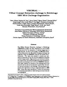
Evidently, whenever τ w becomes of the order of the total stress in the surface layer (this happens, for example, for young wind sea) a considerable enhancement of the Charnock parameter is found, resulting in an efficient momentum transfer from air to water. The consequences of this sea-state-dependent momentum transfer will be discussed in Chapter 7. This finally leaves us with the choice of two unknowns namely αˆ from (3.11) and β m from (3.4). The constant αˆ was chosen in such a way that for old wind sea the Charnock parameter α has the value 0.0185 in agreement with observations collected by Wu (1982) on the drag over sea waves. It should be realised though, that the determination of αˆ is not a trivial task, as beforehand the ratio of wave-induced stress to total stress is simply not known. It requires the running of a wave model. By trial and error the constant αˆ was found to be αˆ = 0.01 . The constant β m is chosen in such a way that the growth rate γ in (3.3) is in agreement with the numerical results obtained from Miles’ growth rate. For β m = 1.2 and a Charnock parameter α = 0.0144 we have shown in Fig. 3.1 the comparison between Miles’ theory and (3.3). In addition observations as compiled by Plant (1982) are shown. Realizing that the relative growth rate γ ⁄ f varies by four orders of magnitude it is concluded that there is a fair agreement between our fit (3.3), Miles’ theory and observations. We remark that the Snyder et al. (1981) fit to their field observations, which is also shown in Fig. 3.1 , is in perfect accordance with the growth rate of the low-frequency waves although growth rates of the high-frequency waves are underestimated. Since the wave-in-



duced stress is mainly carried by the high-frequency waves an underestimation of the stress in the surface layer would result.

Figure 3.1 Comparison of theortical growth rates with observations by Plant (1982. Full line: Miles’ theory; full dots: parametrization of Miles’ theory (3.3); dashed line: the fit by Snyder et al. (1981). We conclude that our parametrization of the growth rate of the waves is in good agreement with the observations. The next issue to be considered is how well our approximation of the surface stress compares with observed surface stress at sea. Fortunately, during HEXOS (Katsaros et al. 1987) wind speed at 10 m height, U 10 , surface stress τ and the one-dimensional frequency spectrum were measured simultaneously so that our parametrization of the surface stress may be verified experimentally. For a given observed wind speed and wave spectrum, the surface stress is obtained by solving (3.7) for the stress τ in an iterative fashion as the roughness length z 0 depends, in a complicated manner, on the stress. Since the surface stress was measured by means of the eddy correlation technique, a direct comparison between observed and modelled stress is possible. The work of Janssen (1992) shows that the agreement is good. It is, therefore, concluded that the parametrized version of quasi-linear theory gives realistic growth rates of the waves and a realistic surface stress. However, the success of this scheme for wind input critically depends on a proper description of the high-frequency waves. The reason for this is that the wave-induced stress depends in a sensitive manner on the high-frequency part of the spectrum. Noting that for high frequencies the growth rate of the waves (3.3) scales with wavenumber as γ∼k

3⁄2

,


(3.12)


and the usual whitecapping dissipation scales as γd ∼ k ,

(3.13)

an imbalance in the high-frequency wave spectrum may be anticipated. Eventually, wind input will dominate dissipation due to wave breaking, resulting in energy levels which are too high when compared with observations. Janssen et al. (1989b) realized that the wave dissipation source function has to be adjusted in order to obtain a proper balance at the high frequencies. The dissipation source term of Hasselmann (1974) is thus extended as follows: 2 k k 2 2 S ds = – C ds 〈 ω〉 ( 〈 k〉 m 0 ) ( 1 – δ ) -------- + δ  -------- N ,  〈 k〉 〈 k〉 

(3.14)

where C ds and δ are constants, m 0 is the total wave variance per square metre, k the wavenumber and 〈 ω〉 and 〈 k〉 are the mean angular frequency and mean wavenumber, respectively. In practice, we take C ds = 4.5 and δ = 0.5 . The choice of the above dissipation source term may be justified as follows. In Hasselmann (1974), it is argued that whitecapping is a process that is weak-in-the-mean, therefore, the corresponding dissipation source term is linear in the wave spectrum. Assuming that there is a large separation between the length scale of the waves and the whitecaps, the power of the wavenumber in the dissipation term is found to be equal to one. For the highfrequency part of the spectrum, however, such a large gap between waves and whitecaps may not exist, allowing the possibility of a different dependence of the dissipation on wavenumber. This concludes the description of the input source term and the dissipation source term due to whitecapping. Although the wind input source function is fairly well-known from direct observations, there is relatively little hard evidence on dissipation. Presently, the only way out of this is to take the functional form for the dissipation in (3.14) for granted and to tune the constants C ds and δ in such a way that the action balance equation (2.24) produces results which are in good agreement with data on fetch-limited growth and with data on the dependence of the surface stress on wave age. In addition, a reasonable dissipation of swell should be obtained. It was decided to follow this method and, after an extensive tuning exercise, the constants C ds and δ were given the values 4.5 and 0.5 while the constant αˆ in the Charnock parameter was given the value 0.01. 3.2.1 Wind gustiness and air density The input source term given in (3.6) and (3.3) assumes homogeneous and steady wind velocity within a model gridbox and during a time-step. Assuming that the wind speed variations with scales much larger than both the spatial resolution and the time step are already resolved by the atmospheric model, we need to include the impact of the wind variability at scales comparable to or lower than the model resolution (which is called wind gustiness). To achieve this, an enhanced input source term with the mean impact of gustiness can be estimated as: ∞

γ ( u* ) = ( u*

2  ( u* – u* )  1 ---------------exp – --------------------- ∫ σ 2π  2σ*  γ ( u* ) du* = –∞ ) *

(3.15)

where u * represents the instantaneous (unresolved) wind friction velocity, σ * is the standard deviation of the friction velocity and the over-barred quantity represents the mean value of the quantity over the whole grid-box/timestep. Note that this is the (gust-free) value obtained from the atmospheric model. The integral above can be approximated using the Gauss-Hermite quadrature as: γ ( u * ) ≅ 0.5 { γ ( u * – σ * ) + γ ( u * + σ * ) }

(3.16)



The magnitude of variability can be represented by the standard deviation of the wind speed. To estimate the standard deviation value, one can use the empirical expression proposed by Panofsky et al. (1977) which can be written as: 1⁄3

zi  σ 10  -------- =  b + 0.5  ----   L  u* 

(3.17)

where σ 10 is the standard deviation of the 10 m wind speed, z i is the height of the lowest inversion, L is the Monin–Obukhov length, and b is a constant representing the background gustiness level that exists all the times irrespective of the stability conditions. The quantity z i ⁄ L , which is a measure for the atmospheric stability, is readily available in the atmospheric model. The impact of the background level of gustiness is already included implicitly in the parameterisations of the atmospheric model as well as in the wave model. Therefore, the constant b value is used as 0 (see Abdalla and Bidlot, 2002). The growth rate of waves is proportional to the ratio of air to water density, ε , as can be seen in (3.3). Under normal conditions, seawater density varies within a very narrow range and, therefore, it can be assumed to be constant. On the other hand, air density has a wider variability and need to be evaluated for better wave predictions. Based on basic thermodynamic concepts, it is possible to compute the air density using the following formula: P ρ air = ----------RT v

(3.18) –1

–1

where P is the atmospheric pressure, R is a constant ( ≈ 287.04 J kg K ) defined as R = R * ⁄ m a , with R * –1 –1 the universal gas constant ( ≈ 8314.36 J kmol K ) and m a is the molecular weight of the dry air –1 ( ≈ 28.966 kg kmol ) and T v is the virtual temperature. The virtual temperature can be related to the actual air temperature, T , and the specific humidity, q , by: T v ≈ ( 1 + 0.6078q )T . In particular, the surface pressure is used for P , the skin temperature is used for T , and the humidity at 2 m height is used for q (see Abdalla and Bidlot, 2002).

3.3 NONLINEAR TRANSFER In Komen et al. (1994) the derivation of the source function S nl , describing the nonlinear energy transfer, was given from first principles. For surface gravity waves the nonlinear energy transfer is caused by four resonantly interacting waves, obeying the usual resonance conditions for the angular frequency and the wave numbers. The evaluation of S nl therefore requires an enormous amount of computation because a three dimensional integral needs to be evaluated. In the past several attempts have been made to try to obtain a more economical evaluation of the nonlinear transfer. The approach that was most succesful to date is the one by Hasselmann et al. (1985). The reason for this is that their parametrization is both fast and it respects the basic properties of the nonlinear transfer, such as conservation of momentum, energy and action, while it also produces the proper high-frequency spectrum. To this end, Hasselmann et al. (1985) constructed a nonlinear interaction operator by considering only a small number of interaction configurations consisting of neighbouring and finite distance interactions. It was found that, in fact, the exact nonlinear transfer could be well simulated by just one mirror-image pair of intermediate range interactions configurations. In each configuration, two wavenumbers were taken as identical k 1 = k 2 = k . The wavenumbers k 3 and k 4 are of different magnitude and lie at an angle to the wavenumber k , as required by the resonance conditions. The second configuration is obtained from the first by reflecting the wavenumbers k 3 and k 4 with respect to the k -axis. The scale and direction of the reference wavenumber are allowed to vary continu-



ously in wavenumber space. The simplified nonlinear operator is computed by applying the same symmetrical integration method as is used to integrate the exact transfer integral (see also Hasselmann and Hasselmann, 1985), except that the integration is taken over a two-dimensional continuum and two discrete interactions instead of five-dimensional interaction phase space. Just as in the exact case the interactions conserve energy, momentum and action. For the configurations ω1 = ω2 = ω ω3 = ω ( 1 + λ ) = ω+

(3.19)

ω4 = ω ( 1 – λ ) = ω– where λ = 0.25 , satisfactory agreement with the exact computations was achieved. From the resonance conditions the angles θ 3 , θ 4 of the wavenumbers k 3 ( k + ) and k 3 ( k – ) relative to k are found to be θ 3 = 11.5° , θ 4 = – 33.6° . The discrete interaction approximation has its most simple form for the rate of change in time of the action density in wavenumber space. In agreement with the principle of detailed balance, we have N –2 ∂ – 8 19 2 ----- N + = +1 C g f [ N ( N + + N – ) – 2 N N + N – ]∆k , ∂t N– +1

(3.20)

where ∂N ⁄ ∂t , ∂ N + ⁄ ∂t , ∂ N – ⁄ ∂t are the rates of change in action at wavenumbers k , k + , k – due to the discrete interactions within the infinitesimal interaction phase-space element ∆k and C is a numerical constant. The net source function S nl is obtained by summing equation (3.20) over all wavenumbers, directions and interaction configurations. For a JONSWAP spectrum the approximate and exact transfer source functions have been compared in Komen et al. (1994). The nonlinear transfer rates agree reasonably well, except for the strong negative lobe of the discreteinteraction approximation. This feature is, however, less important for a satisfactory reproduction of wave growth than the correct determination of the positive lobe which controls the down shift of the spectral peak. The usefulness of the discrete-interaction approximation follows from its correct reproduction of the growth curves for growing wind sea. This is shown in Fig. 3.2 where a comparison is given of fetch-limited growth curves for some important spectral parameters computed with the exact nonlinear transfer, or, alternatively, with the discreteinteraction approximation. Evidence of the stronger negative lobe of the discrete interaction approximation is seen through the somewhat smaller values of the Phillips constant α p . The broader spectral shape corresponds with the smaller values of peak enhancement γ for the parametrized case. On the other hand, the agreement of the more important scale parameters, the energy ε * and the peak frequency ν * is excellent (note that, as always, an asterix denotes nondimensionalisation of a variable through g and the friction velocity u * ).



Figure 3.2 Comparison of fetch-growth curves for spectral parameters computed using the exact form and the discrete interaction approximation of S nl . All variables are made dimensionless using u * and g . The above analysis is made for deep water. Numerical computations by Hasselmann and Hasselmann (1981) of the full Boltzmann integral for water of arbitrary depth have shown that there is an approximate relation between transfer rates in deep water and water of finite depth: for a given frequency-direction spectrum, the transfer for finite depth is identical to the transfer for infinite depth, except for a scaling factor R : S nl ( finite depth ) = R ( kh )S nl ( infinite depth ) ,

(3.21)

where k is the mean wavenumber. This scaling relation holds in the range kh > 1 , where the exact computations could be closely reproduced with the scaling factor 5.5 5x 5x R ( x ) = 1 + -------  1 – ------ exp  – ------ ,  4 x  6

(3.22)

with x = ( 3 ⁄ 4 )kh . This approximation is used therefore in the WAM model.

3.4 THE ENERGY BALANCE IN A GROWING WIND SEA Having discussed the parametrization of the physics source terms we now proceed with studying the impact of wind input, nonlinear interaction and whitecap dissipation on the evolution of the wave spectrum for the simple case of a duration-limited wind sea. To this end we numerically solved equation (2.24) for infinite depth and a constant



wind of approximately 18 m/s, neglecting currents and advection. Typical results are shown in Fig. 3.3 for a young wind sea ( T = 3 h ) and in Fig. 3.4 for an old wind sea ( T = 96 h ). In either case the directional averages of S nl , S in and S ds are shown as functions of frequency. First of all we observe that, as expected from our previous discussions, the wind input is always positive, and the dissipation is always negative, while the nonlinear interactions show a three lobe structure of different signs. Thus, the intermediate frequencies receive energy from the airflow which is transported by the nonlinear interactions towards the low and high frequencies.

Figure 3.3 The energy balance for young duration-limited wind sea.

Figure 3.4 The energy balance for old wind sea.



Concentrating for the moment on the case of young wind sea, we immediately conclude that the one-dimensional –4 frequency spectrum in the ‘high’-frequency range must be close to f , because the nonlinear source term is quite small (see the discussion in § II.3.10 of Komen et al. (1994) on the energy cascade caused by the four-wave interactions and the associated equilibrium shape of the spectrum). We emphasize, however, that because of the smallness of S nl it cannot be concluded that the nonlinear interactions do not control the shape of the spectrum in this range. On the contrary, a small deviation from the equilibrium shape would give rise to a large nonlinear source term which will drive the spectrum back to its equilibrium shape. The role of wind input and dissipation in this relaxation process can only be secondary because these source terms are approximately linear in the wave spectrum. The combined effect of wind input and dissipation is more of a global nature in that they constrain the magnitude of the energy flow through the spectrum (which is caused by the four-wave interactions). At low frequencies we observe from Fig. 3.3 that the nonlinear interactions maintain an ‘inverse’ energy cascade by transferring energy from the region just beyond the location of the spectral peak (at f ≈ 0.12 Hz ) to the region just below the spectral peak, thereby shifting the peak of the spectrum towards lower frequencies. This frequency downshift is, however, to a large extent, determined by the shape and magnitude of the spectral peak itself. For young wind sea, having a narrow peak with a considerable peak enhancement, the rate of downshifting is significant while for old wind sea this is much less so. During the course of time the peak of the spectrum gradually shifts towards lower frequencies until the peak of the spectrum no longer receives input from the wind because these waves are running faster than the wind. Under these circumstances the waves around the spectral peak are subject to a considerable dissipation so that their wave steepness becomes reduced. Consequently, because the nonlinear interactions depend on the wave steepness, the nonlinear transfer is reduced as well. The peak of the positive lowfrequency lobe of the nonlinear transfer remains below the peak of the spectrum, where it compensates the dissipation. As a result, a quasi-equilibrium spectrum emerges. The corresponding balance of old wind sea is shown in Fig. 3.4 . The nature of this balance depends on details of the directional distribution (see Komen et al., 1984 for additional details). The question of whether an exact equilibrium exists appears of little practical relevance. For old wind sea the timescale of downshifting becomes much larger than the typical duration of a storm. Thus, although from the present knowledge of wave dynamics it cannot be shown that wind-generated waves evolve towards a steady state, for all practical purposes they do! This concludes our discussion of the parametrization of the physics source terms. Before presenting a discussion of the numerical scheme we have used to solve the action balance equation we shall first describe the data assimilation scheme.




CHAPTER 4 An optimal interpolation scheme for assimilating altimeter data into the WAM model Table of contents 4.1 Introduction 4.2 Wave height analysis 4.2.1 The analysed wave spectrum 4.2.2 Retrieval of a wind sea spectrum 4.2.3 Retrieval of a swell spectrum 4.2.4 The general case

4.1 INTRODUCTION The optimal interpolation method described in this section was developed for the WAM model and is operational at ECMWF (Lionello et al., 1992). Similar single-time level data assimilation techniques for satellite altimeter wave heights have been applied by Janssen et al. (1987, 1989b), Hasselmann et al. (1988), Thomas (1988) and Lionello et al. (1992). In this case we are dealing with the well-known problem that there are more degrees of freedom than observations because the altimeter only provides us with significant wave height. Thus, instead of estimating the full state vector, we estimate only the significant wave height field H (the index S in the notation for the significant wave height f is dropped in the following discussion). The data vector d consists then of the first-guess model wave heights, o interpolated to the locations of the altimeter observations, while d are the actually observed altimeter wave heights. The assimilation procedure consists of two steps: • first an analysed field of significant wave heights is created by optimum interpolation, in accordance with the general oi approach outlined in Lorenc (1981) and with appropriate assumptions regarding the error covariances; then • this field is used to retrieve the full two-dimensional wave spectrum from a first-guess spectrum, introducing additional assumptions to transform the information of a single wave height measurement into separate corrections for the wind sea and swell components of the spectrum. The problem of using wave height observations for correcting the full two-dimensional spectrum was first considered by Hasselmann et al. (1988) and Bauer et al. (1992), who assimilated SEASAT altimeter wave heights into the WAM model by simply applying a constant correction factor, given by the ratio of altimeter and model wave heights, to the entire spectrum. A shortcoming of this method was that the wind field was not corrected. Thus although swell corrections were retained for several days, the corrected wind sea relaxed back rapidly to the original incorrect state due to the subsequent forcing by uncorrected winds. Janssen et al. (1987) removed this shortcoming by extending the method to include wind corrections, but nevertheless achieved only short relaxation times due to the choice of an insufficient correlation scale (the corrections were essentially limited to a single grid point). This



was remedied in later versions of the scheme described below. As in most of these schemes, the present method corrects the two-dimensional spectrum by introducing appropriate rescaling factors to the energy and frequency scales of the the wind sea and swell components of the spectrum, and also updates the local forcing wind speed. The rescaling factors are computed for two classes of spectra: wind sea spectra, for which the rescaling factors are derived from fetch and duration growth relations, and swell spectra, for which it is assumed that the wave steepness is conserved. All observed spectra are assigned to one of these two classes. This restriction will be removed in the planned extension of the scheme to include SAR wave mode data.

4.2 WAVE HEIGHT ANALYSIS a

a

First, an analysis of the significant wave height field H = ( H i ) is created by optimum interpolation (cf. Lorenc, 1981): n obs a

f

Hi = Hi +

∑ W ij ( H j – H j ) , o

f

(4.1)

j=1 o

f

where H denotes the significant wave height field observed by the altimeter and H is the first-guess significant wave height field computed by the WAM model. Since long-term statistics of the prediction and observational error covariance matrices equation were not available, empirical expressions were taken:  σi  xi – x j  f o f - and σ ij = δ ij  -----f  . σ ij = σ exp  – -----------------  L  σi  o

(4.2)

Good results were obtained for a correlation length L = 1650 km . This is consistent with the optimal scale length found by Bauer et al. (1992) using a triangular interpolation scheme. However, at ECMWF we use a much smaller value of 300 km. 4.2.1 The analysed wave spectrum In the next step, the full two-dimensional wave spectrum is retrieved from the analysed significant wave height fields. Two-dimensional wave spectra are regarded either as wind sea spectra, if the wind sea energy is larger than 3/4 times the total energy, or, if this condition is not satisfied, as swell. a

In both cases an analysed two-dimensional wave spectrum F ( f , θ ;x, t ) is computed from the first-guess wave a f spectrum F ( f , θ ;x, t ) and the optimally interpolated wave heights H i by rescaling the spectrum with two scale parameters A and B : a

f

F ( f , θ ) = AF B ( f , θ ) .

(4.3)

Different techniques are applied to compute the parameters A and B for wind sea or swell spectra. 4.2.2 Retrieval of a wind sea spectrum The parameters A and B in equation (4.3) can be determined from empirical duration-limited growth laws relat4 2 ing, in accordance with Kitaigorodskii’s (1962) scaling laws, the nondimensional energy ε * = u * ε ⁄ g (where 2 ε = ( H ⁄ 4 ) ), mean frequency f * = u * f ⁄ g and duration T * = u * T ⁄ g . Specifically, we take the following


Chapter 4 ‘An optimal interpolation scheme for assimilating altimeter data into the WAM model’

relations (which deviate considerably from the ones proposed by Lionello et al. (1992)): 1.143

t* ε * ( t * ) = 1673 --------------------------------------6 t * + 1.049 × 10

,

(4.4)

and – 4 – 2.87

ε * ( f * ) = 7.24 × 10 f *

.

(4.5)

The mean frequency is preferred to the peak frequency because its computation is more stable. Since the first-guess friction velocity was used to generate the waves and the first-guess wave height is known, an estimate of the duration T of the wind sea can be derived from the duration-limited growth laws. Assuming this estimated duration is correct, the analysed wave height yields from the growth laws, equations (4.4) and (4.5), best estimates of the frica a tion velocity u * and mean frequency f . The analysed wave height and mean frequency determine then the two parameters A and B : 2

a  H a f -----a =  f  B and B = -----f . H  f

(4.6)

The corrected best-estimate winds are then used to drive the model for the rest of the wind time step. In a comprehensive wind and wave assimilation scheme, the corrected winds should be also inserted into the atmospheric data assimilation scheme to provide an improved wind field in the forecast model. 4.2.3 Retrieval of a swell spectrum A spectrum is converted to swell and begins to decay at the edge of a storm, before dispersion has separated the swell into spatially distinct frequencies. One can therefore distinguish between a nonlinear swell regime close to the swell source and a more distant linear regime, where dispersion has reduced the swell wave slopes to a level at which nonlinear interactions have become negligible. Because of these complexities, and also because of a lack of adequate data, there exist no empirical swell decay curves comparable to the growth curves in the wind sea case. However, Lionello and Janssen (1990) showed that for the WAM model swell spectra the average wave steepness, H s = 〈 k〉 -----8π

(4.7)

is approximately the same for all spectra at the same decay times, despite the wide range of significant wave heights and mean frequencies of their data set. Assuming that the effective decay time and therefore the wave steepness is not affected by the correction of the wave spectrum, the scale factors are then given by f 1⁄2

a

B = (H ⁄ H ) a

f 2

A = B( H ⁄ H ) .

(4.8) (4.9)

Intuitively, this approach appears reasonable, because a more energetic spectrum will generally also have a lower peak frequency, and increasing the energy without decreasing the peak frequency produces a swell of unrealistic steepness. Since the swell spectrum is not related to the local stress, and only the local wind field is corrected in



the assimilation scheme, the wind field is not updated in the case of swell. 4.2.4 The general case It was shown in Lionello et al. (1992) that the wind sea and swell retrieval scheme works well for simple cases or pure wind sea or swell. If the spectrum consists of a superposition of wind sea and swell, and the wind sea is well separated from the swell, the wind sea and swell correction methods can, in principle, still be applied separately to the two components of the spectrum. In this case, however, one needs to introduce additional assumptions regarding the partitioning of the total wave height correction between wind sea and swell. The arbitrariness of the present and similar methods of distributing a single wave height correction over the full two-dimensional wave spectrum could presumably be partially alleviated by using maximum likelihood methods based on a large set of observed data, which is now becoming available through ERS-1 . However, a more satisfactory solution is clearly to assimilate additional data, such as two-dimensional SAR spectral retrievals, to overcome the inherently limited information content of altimeter wave height data.




CHAPTER 5 Numerical scheme Table of contents 5.1 Introduction 5.2 Implicit integration of the source functions 5.3 Advective terms and refraction 5.4 Boundary conditions and grid nesting

5.1 INTRODUCTION In this section we discuss the numerical aspects of the solution of the action balance equation as implemented in the ECMWF version of the WAM model. Although, thus far, we have discussed the transport equation for gravity waves for the action density, because this is the most natural thing to do from a theoretical point of view, the actual WAM model is formulated in terms of the frequency-direction spectrum F ( f , θ ) of the variance of the surface elevation. The reason for this is that in practical applications one usually deals with surface elevation spectra, because these are measured by buoys. The relation between the action density and the frequency spectrum is straightforward. It is given by F ( ω, θ ) = σN ( ω, θ ) ,

(5.1)

where σ is the intrinsic frequency (see also equation (2.4)). This relation is in accordance with the analogy between wave packets and particles, since particles with action N have energy σN and momentum kN . The continuous wave spectrum is approximated in the numerical model by means of step functions which are constant in a frequency-direction bin. The size of the frequency-direction bin depends on frequency. A distinction is being made between a prognostic part and a diagnostic part of the spectrum. The prognostic part of the spectrum has KL directional bands and ML frequency bands. These frequency bands are on a logarithmic scale, with ML – 1 ∆f ⁄ f = 0.1 , spanning a frequency range f max ⁄ f min = ( 1.1 ) . The logarithmic scale has been chosen in order to have uniform relative resolution, and also because the nonlinear transfer scales with frequency. The starting frequency may be selected arbitrarily. In most global applications the starting frequency f 0 is 0.042 Hz, the number of frequencies ML is 25 and the number of directions KL is 24 ( 15° resolution). For closed basins, such as the Mediterranean Sea where low-frequency swell is absent, a choice of starting frequency f 0 of 0.05 Hz is sufficient. The present version of the ECMWF wave prediction system has 24 directions and 30 frequencies, with starting frequency f 0 = 0.035 Hz . –5

Beyond the high-frequency limit f hf of the prognostic region of the spectrum, an f tail is added, with the same directional distribution as the last band of the prognostic region. The diagnostic part of the spectrum is therefore given as f –5 F ( f , θ ) = F ( f hf , θ )  ------- for f > f hf .  f hf

(5.2)



In the ECMWF version of the WAM model the high-frequency limit is set as f hf = min { f max, 2.5 〈 f 〉 } .

(5.3)

Thus, the high-frequency extent of the prognostic region is scaled by the mean frequency 〈 f 〉 . A dynamic highfrequency cut-off, f hf , rather than a fixed cut-off at f max is necessary to avoid excessive disparities in the response time scales within the spectrum. A diagnostic tail needs to be added for f > f hf to compute the nonlinear transfer in the prognostic region and also –4 to compute the integral quantities which occur in the dissipation source function. Tests with an f tail show that (apart from the calculation of the wave-induced stress) the results are not sensitive to the precise form of the diagnostic tail. The contribution to the total energy from the diagnostic tail is normally negligible. Because observations –5 seem to favour an f power law (Birch and Ewing, 1986, Forristall, 1981, Banner, 1990) this power law is used for the high-frequency part of the spectrum. The prognostic part of the spectrum is obtained by numerically solving the energy balance equation. We will now discuss the different numerical schemes and time steps that are used to integrate the source functions and the advective terms of the transport equation.

5.2 IMPLICIT INTEGRATION OF THE SOURCE FUNCTIONS An implicit scheme was introduced for the source function integration to enable the use of an integration time step that was greater than the dynamic adjustment time of the highest frequencies still treated prognostically in the model. In contrast to first and second generation wave models, the energy balance of the spectrum is evaluated in detail up to a high cut-off frequency. The high-frequency adjustment time scales are considerably shorter than the evolution time scales of the energy-containing frequency bands near the peak of the spectrum, in which one is mainly interested in modelling applications. Thus, in the high-frequency region it is sufficient to determine the quasi-equilibrium level to which the spectrum adjusts in response to the more slowly changing low-frequency waves, rather than the time history of the short time scale adjustment process itself. An implicit integration scheme whose time step is matched to the evolution of the lower frequency waves meets this requirement automatically: for low-frequency waves, the integration method yields, essentially, the same results as a simple forward integration scheme, while for high frequencies the method yields the (slowly changing) quasi-equilibrium spectrum (WAMDI, 1988). The original WAM model used a time-centred implicit integration scheme, but Hersbach and Janssen(1999) found that numerical noise occurred which may be avoided by a two-time level, fully implicit approach. The fully implicit equations (leaving out the advection terms) are given by F n + 1 = F n + ∆tS n + 1 ,

(5.4)

where ∆t is the time step and the index n refers to the time level. If S n + 1 depends linearly on F n + 1 , equation (5.4) could be solved directly for the spectrum F n + 1 at the new time step. Unfortunately, none of the source terms are linear. We therefore introduce a Taylor expansion ∂S n S n + 1 = S n + ---------- ∆F + . . . . ∂F

(5.5)

The functional derivative in (5.5) (numerically a discrete matrix M n ) can be divided into a diagonal matrix Λ n and a nondiagonal residual N n ,


Chapter 5 ‘Numerical scheme’

∂S ---------n- = M n = Λ n + N n . ∂F

(5.6)

Substituting (5.5) and (5.6) into (5.4), realizing, in addition, that the source term S may depend on the friction velocity u * at time level n + 1 , we obtain n+1

1 – ∆t { Λ n ( u *

n+1

) + N n ( u*

n+1

) } ∆F = ∆tS n ( u *

)

(5.7)

with ∆F = F n + 1 – F n . A number of trial computations indicated that the off diagonal contributions were generally small if the time step was not too large. Disregarding these contributions, the matrix on the left-hand side can be inverted, yielding for the increment ∆F , n+1

∆F = ∆tS n ( u *

n+1

) 1 – ∆tΛ n ( u *

)

–1

.

(5.8)

Nevertheless, in practice numerical instability is found in the early stages of wave growth. These are either caused by the neglect of the off diagonal contributions or by the circumstance that the solution is not always close to the attractor of the complete source function. Therefore a growth limitation needs to be imposed. In the ECMWF version of WAM a variant of the growth limiter of Hersbach and Janssen(1999) is used: the maximum increment in the spectrum, ∆F max , is given by ∆F

–7

max

= 5 × 10 gu * f

–4

〈 f 〉 ∆t

(5.9)

For a typical test case, good agreement was obtained between an explicit integration with a time step of 1 minute and the implicit scheme with only diagonal terms for time steps up to about 20 minutes.

5.3 ADVECTIVE TERMS AND REFRACTION The advective and refraction terms in the energy balance equation have been written in flux form. We shall only consider, as an example, the one-dimensional advection equation ∂ ∂ ----- F = – ------ Φ , ∂t ∂x

(5.10)

with flux Φ = c g F , since the generalization to four dimensions λ , φ , θ and ω is obvious. Two alternative propagation schemes were tested, namely a first order upwinding scheme and a second order leap frog scheme (for an account of the numerical schemes of the advection form of the energy balance equation see WAMDI , 1988). The first-order scheme is characterized by a higher numerical diffusion, with an effective diffusion coefficient 2 D ∼ ∆x ⁄ ∆t , where ∆x denotes grid spacing and ∆t is the time step. For numerical stability the time step must satisfy the inequality ∆t < ∆x ⁄ c g , so that D > c g ∆x . The advection term of the second-order scheme has a smaller, inherent, numerical diffusion, but suffers from the drawback that it generates unphysical negative energies in regions of sharp gradients. This can be alleviated by including explicit diffusion terms. In practice, the explicit diffusion required to remove the negative side lobes in the second order scheme, is of the same order as the implicit numerical diffusion of the first order scheme, so that the effective diffusion is generally comparable for both schemes.



As shown in WAMDI (1988) both schemes have similar propagation and diffusion properties. An advantage of the second order scheme is that the lateral diffusion is less dependent on the propagation direction than in the first order scheme, which shows significant differences in the diffusion characteristics for waves travelling due south-north or west-east compared with directions in between. The first order scheme has the additional problem that there is excessive shadowing behind islands when waves are propagating along the coordinate axes. However, these undesirable features in the first order upwinding scheme may be alleviated by rotating the spectra by half its angular resolution, in such a way that no spectral direction coincides with the principle axes of the spatial grid. In general, the differences between the model results using first or second order propagations methods were found to be small, but there is a preference for the first order scheme because of its efficiency and simplicity.

Figure 5.1 Definition of grid points for first-order upwinding scheme. Historically, the main motivation for considering the second order scheme in addition to the first order scheme was not to reduce diffusion, but to be able to control it. In contrast to most other numerical advection problems, an optimal propagation scheme for a spectral wave model is not designed to minimize the numerical diffusion, but rather to match it to the finite dispersion associated with the finite frequency-direction spectral resolution of the model (SWAMP , 1985, appendix B). In this context, it should be pointed out that an ideal propagation scheme would give poor results for sufficiently large propagation times, since it would not account for the dispersion associated with the finite resolution in frequency and direction (the so-called garden sprinkler effect). Now, the dispersion due to the different propagation velocities of the different wave components within a finite frequency-direction bin increases linearly with respect to propagation time or distance, whereas most propagation schemes yield a spreading of the wave groups which increases with the square root of the propagation time or distance. However, Booij and Holthuijsen (1987) have shown that linear spreading rates may be achieved by introducing a variable diffusion coefficient proportional to the age of the wave packets. This idea has been tested in the context of a third generation wave model by Chi Wai Li (1992) and Tolman (2000) who uses an averaged age of the wave packets per ocean basin. To summarize our discussion, we have chosen the first order upwinding scheme because it is the simplest scheme to implement (requiring less computer time and memory) and because in practice it gives reasonable results. Applied to the simple advection scheme in flux form (5.10) we obtained the following discretization, where for the definition of grid points we refer to Fig. 5.1 . The rate of change of the spectrum ∆F j in the j th grid point is given by ∆t ∆F j = – ------- ( Φ j + 1 ⁄ 2 – Φ j – 1 ⁄ 2 ) , ∆x

(5.11)

where ∆x is the grid spacing and ∆t the propagation time step, and 1 1 Φ j + 1 ⁄ 2 = --- [ v j + v j ]F j + --- [ v j – v j ]F j + 1 , 2 2


(5.12)

Chapter 5 ‘Numerical scheme’

where v j = 0.5 ( c g, j + c g, j + 1 ) is the mean group velocity and the flux at j – 1 ⁄ 2 is obtained from (5.12) by replacing j + 1 ⁄ 2 with j – 1 ⁄ 2 . The absolute values of the mean speeds arise because of the upwinding scheme. For example, for flow going from the left to the right the speeds are positive and, as a consequence, the evaluation of the gradient of the flux involves the spectra at grid points j – 1 and j .

Figure 5.2 Irregular grid for North Atlantic area. We furthermore remark that one could consider using a semi-Lagrangian scheme for advection. This scheme is gaining popularity in meteorology because it does not suffer from the numerical instabilities which arise in conventional discretization schemes when the time step is so large that the Courant-Friedrichs-Levy (CFL) criterion is violated. The wave model community has, so far, not worried too much about this problem because advection is a relatively inexpensive part of the computations. In addition, in most applications, the propagation time is larger or equal to the source time step, which is usually 20 min. According to the CFL criterion, short propagation time steps (less than, say, 10 min) are only required for very high resolution ( ∆x < 20 km ). But in these circumstances the advection will induce changes in the physics on a short time scale, so that it is advisable to decrease the source time step accordingly. Therefore, in the WAM model, the source time step is always less than or equal to the propagation time step. We finally comment on the so-called pole problem in the case of of the use of spherical coordinates. When moving towards the poles, the distance in the latitudinal direction decreases. Clearly, close to the poles violation of the \ CFL criterion occurs. In the ECMWF version of the WAM model this problem is solved by choosing an irregular spherical grid in such a way that the distance in the latitude direction is more or less fixed to its value at the equator.



An example of such a grid from the present operational ECMWF WAM model is shown in Fig. 5.2 . The advection scheme is still formulated in terms of spherical coordinates but the gradient in the longitudinal fluxes is evaluated by linear interpolation of the fluxes from the closest neighbours. The additional advantages of the use of an irregular spherical grid is a reduction in the total number of grid points by 30%, giving a substantial reduction in the cpu consumption.

5.4 BOUNDARY CONDITIONS AND GRID NESTING Normally the wave model grid is surrounded by land points. Therefore, the natural boundary conditions are no energy flux into the grid and free advection of energy out of the grid at the coastline. The generation and propagation of ocean waves covers a wide range of space and time scales. In the open ocean, the scale of a wind sea system is determined by the size of a depression, which typically has scales of the order of 1000 km. On the other hand, near the coast, the scale of a wave system is determined by the coastal geometry and bottom topography, which have usually much smaller scales. A wave model which covers all scales uniformly is not practicable because of computer limitations. In addition, running a high-resolution wave model for the open ocean seems a waste of computer time. There are several ways out of this problem. One approach would be to run a wave model with a variable grid, having a high resolution whenever needed (for example near the coast) and having a coarse resolution in the open ocean. So far this approach has not been followed. The WAM model was developed with the practical application in mind of running a global ocean wave model at ECMWF and running limited area models at the European National Weather Centres. Therefore, preference was given to another solution, in which one has the option to run the model on nested grids. This gives the opportunity to use results of a coarse mesh model from a large region in a fine mesh regional model. Several successive levels of nesting may be necessary. The two-dimensional spectra computed by the coarse mesh model are saved at grid points which are on the boundary of the limited area, high-resolution grid. These spectra are then interpolated in space and time to match the high resolution at the grid boundaries. It should be pointed out, however, that a straightforward linear interpolation of spectra gives problems because the interpolated spectra are usually not well balanced, resulting in their rejection when used as boundary conditions for a fine mesh run. To circumvent this problem, the following interpolation procedure is used. Instead of linearly interpolating the spectra from the adjacent points of the coarse grid directly, we rescale these spectra in such a way that the rescaled spectrum has the same mean frequency, mean wave direction and wave energy as found from a linear interpolation of these mean quantities to the fine mesh grid point. The wave spectrum at the fine mesh grid point is then found by linearly interpolating the rescaled spectra. This procedure seems to give satisfactory results.




CHAPTER 6 The WAM-model software package Table of contents 6.1 Introduction 6.2 Massive Parallel Computing 6.3 Pre-processing programs 6.4 Processing programs 6.5 Post-processing programs 6.6 ECMWF Post-Processing

6.1 INTRODUCTION

Figure 6.1 Structure of the model grid. The WAM model development was finished in the early 1990’s. Since then there has been continuous effort at ECMWF to streamline the software in areas such as IO, archiving, vectorization and to adapt the code to the new massive parallel (vector) machines. Nevertheless, many of the original features of the WAM model have been retained. These are described below, followed by a description of the additional features that have been introduced at ECMWF. The original WAM model software that has been developed over a period of seven years (1985-1992) is fairly gen-



eral. Spectral resolution and spatial resolution are flexible and the model can be run globally or regionally with open and closed boundaries. Open boundaries are important in case one wishes to use results from a coarse resolution run as boundary conditions for a fine mesh, limited area run. Options such as shallow water, depth refraction or current refraction may be chosen. In this subsection we shall briefly describe the wave model software with emphasis on flexibility and universality. Before doing this, we shall first discuss some design choices. The model was developed with an important application in mind, namely for predicting operationally waves over the whole globe. With a modest spatial resolution of 3° (resulting in approximately 4000 grid points) and 25 frequencies and 12 directions, it follows that about 1.2 million equations have to be solved. Since the most expensive part of the numerical code, the nonlinear source term, cannot be vectorized, vectorization is achieved over the grid points, which are placed in the innermost loop. In order to make this loop as long as possible, a mapping from the two-dimensional spherical grid to a one-dimensional array is performed. If there are no limitations to the amount of internal memory of the computer, the most efficient procedure is to convert the entire global grid to a single onedimensional array. In practice, however, there may be restrictions on the amount of memory to be used. For example, in the early days of the WAM model development, the model was tested on a Cray 1S with an internal memory of only 750,000 words. Clearly, the full model grid would not fit into this small memory. It was, therefore, decided to split up the globe in blocks of NIBLO grid points. Typically, NIBLO = 512. The blocks are set up in such a way that the north and south boundaries are either land or open ocean, whereas the east and west boundaries are land, periodic (this occurs, for instance, in the southern ocean), or open ocean (for nesting). In order to allow waves to propagate oss the north or south boundaries of a block, the blocks overlap by a number of latitudes, depending on the propagation scheme. Since we have chosen a first order upwinding scheme, which involves only two neighbouring grid points, the number of overlapping latitudes is two. The computations are done from the last but one southerly latitude to the last but one most northerly latitude (see also Fig. 6.1 and Günther et al., 1991). Although loading only one block at a time circumvents the problem of the limited memory, the drawback of this approach is that extensive input-output (IO) operations are needed. After performing the computations on block IG, the results have to be written to disc and the results of the previous time step of block IG + 1 have to be read before the computations on block IG + 1 may be started. To avoid waiting for IO, an IO scheme is used that allows for simultaneously writing results of block IG – 1, reading results of the previous time step of block IG + 1, while performing calculations on block IG. The block structure combined with this IO scheme yields a very efficient and flexible wave model code. With the preprocessing program PREPROC one may lay out a block structure according to one’s own choice. The later generation of computers, such as the CRAY-YMP, allowed the whole globe to be loaded into the core of the computer, hence a one block structure may be chosen. This is, however, not always the optimal choice when high resolution applications are considered and/or when the wave model is coupled to another model, for example an atmospheric model or a storm-surge model. Later generation of computers are based on the concept of massive parallel computing. In this context it is important to distinguish between memory shared and memory distributed machines. Machines such as the CRAY-YMP and the CRAY-C90 are examples of shared memory machines. By using Macrotasking it was relatively straightforward to develop a version of the WAM model that utilised more processors in an efficient way. Note that there are limits to the number of processors to be used, because each processor requires a sufficient amount of work. Therefore, a low resolution version of the WAM model, such as the 1.5 deg model, could only perform efficiently on about 4 processors, while the high resolution, 55 km, version ran still efficiently on 16 processors. The present generation of computers either are memory distributed machines or have memory distribution over nodes while per node the processors share the memory. In general, a memory distributed machine requires a different approach which is described in the next subsection.


Chapter 6 ‘The WAM-model software package’

6.2 MASSIVE PARALLEL COMPUTING Memory distributed machines such as the Fujitsu vpp series require the introduction of message passing between processors (known as processing elements (PE’s)). Therefore, one PE can send a message which is received by one or more other PE’s. In its very basic implementation, the message is nothing more than a one-dimensional array of a given type containing values that are needed by the other PE(s) plus the necessary information about the sender and receiver. For a succesful message exchange both send and receive should be completed. Message passing in the ECMWF version of the WAM model was introduced in 1996 based on the message passing library MPELIB. This newly developed code can also run on non distributed memory machines and on a single PE.

Information at those grid points may be needed to compute the advection at grid points in subregion N.

N+1

N

X

X

X

X

X

X

X

X

X

X

X

X

X

X

X

X

X

X

X

X

B

1

X

N-1

A

Increasing index for the sea-point arrays

Information at those grid points may be needed to compute the advection at grid points in subregion N.

Figure 6.2 Domain decomposition. When running in parallel it is important to have an even distribution of work over the PE’s in order to avoid load



unbalance. In the case of the WAM model it comes down to splitting the global computation domain into regions of equal size, keeping in mind that information is only locally known on each PE and can only be exchanged with the other PE’s via message passing(which is a slower process than computing). In the present setting the number of processors is determined at run time. Once the message passing program starts simultaneously on all assigned PE’s, the parallel environment and the message passing protocol is initialized. Also, the total number of PE’s is determined as well as the logical PE on which the code is run. This initialisation procedure is done in CHIEF, or any other start up main program which calls the WAM model. Once the total number of PE’s is known, MPDECOMP is called to set up an even decomposition of the total grid into one sub domain per PE. Since the global grid is mapped onto a one-dimensional sea point array following increasing latitude lines, the sub domains are chosen to be consecutive segments of the full sea point array (cf. Fig. 6.2 ). The length of each segment is determined by the requirement that the work is distributed in an even manner over the given number of PE’s. Thus, each PE will only perform the integration of the source functions of the energy balance equation of one subdomain. However, the upwind scheme which solves the advection term, uses neighbouring grid points in the 2-D grid that might belong to another subdomain. The necessary information from the other PE’s needed to evaluate the spatial derivatives of the energy flux are obtained through message passing. Here, the message is constructed using the geometrical rules displayed in Fig. 6.2 , and is similar in spirit as the method that was developed for the multi-block version of the WAM model. An important difference is, however, that the domain composition is done at run time, allowing more flexibility. This completes our discussion regarding the design of the WAM model. The remainder of this subsection is devoted to the model system. A more detailed description of this may be found in the manual wamodel cycle 4 by Günther et al. (1991). The model system consists of three parts: 1) pre-processing programs, 2) processing programs, 3) post-processing programs. The original WAM model is designed to run as a module of a more general system or as a stand-alone program. The pre-processing programs generate the model grid, bathymetry-dependent dispersion relation, etc. Postprocessing programs are provided for archiving and for further analysis of the model output.

6.3 PRE-PROCESSING PROGRAMS Two pre-processing programs are provided: 1) PREPROC, 2) PRESET. The program PREPROC generates all time-independent information for the wave model. Starting from a regional or global topographic data set the model grid is created in the form required for the model. The standard model grid is a latitude-longitude grid, which may be regular or irregular, but Cartesian grids can also be chosen. Frequency, angular and group velocity arrays are generated. If the current refraction option is activated, PREPROC expects a current data set and interpolates the data onto the model grid. A number of model constants and matrices, such as the surface stress as a function of wind speed and wave-induced stress, are pre-computed and stored together with the model grid, frequency and angular information and the currents in two output files. If nested grids are generated, the information for the output, input and interpolation of boundary spectra are presented and stored in separate files



for the coarse and fine mesh models. PRESET generates an initial wave field for a wave model cold start in the event that no appropriate initial conditions are available. Controlled by the user input of PRESET, either the same initial JONSWAP spectrum is used at all ocean grid points, or the initial spectra are computed from the local initial winds, according to fetch laws with 2 a cos directional distribution.

6.4 PROCESSING PROGRAMS There are two processing programs, namely 1) CHIEF, 2) BOUINT. The program BOUINT is used for nested grids. It interpolates, in time and space, the output spectra from a coarse grid model run onto the fine grid along the boundaries of the coarse and fine grids. CHIEF is the shell program of the stand-alone version of the wave model which calls the subroutine version WAVEMDL of the wave model. All time-dependent variables and user defined parameters are set, the wind fields are transformed to the wave model grid and the transport equation is integrated over a chosen period. The program uses the output files of PREPROC as set-up files and the files generated by PRESET or a previous model run as initial values. A wind input file has to be provided by the user. All additional information must be defined in the user input file. The model can be integrated with independently chosen propagation, source term and wind time steps, under the restriction that all time step ratios must be an integer, or the inverse of an integer. A number of model options and parameters may be selected by the user in the program input. The following model options are implemented: 1) Cartesian or spherical propagation, 2) deep or shallow water, 3) with or without depth refraction or with depth and current refraction, 4) nested grids, 5) time interpolation of winds, or no time interpolation, 6) model output at regular intervals, or through a list, 7) printer and/or file output of selected parameters. All run-time-dependent files are fetched dynamically and follow a fixed file name convention. The user has control over directory names and paths through the model input. If selected, model results are saved in four files. These files contain: 1) gridded output fields of significant wave height, mean wave direction, mean frequency, friction velocity, wave direction, peak frequency, drag coefficient and normalized wave-induced stress, 2) gridded output field of swell parameters such as wave height, swell direction, mean wind-wave direction and mean swell frequency, 3) spectra at selected grid points, 4) swell spectra at selected grid points.



Figure 6.3 Flow chart of program CHIEF. A comprehensive view of the program CHIEF, which is clearly the most important part of the model system, is given in the flow chart of Fig. 6.3 . We need not discuss details here and only highlight the main points. The subroutine INITMDL is only called once. It reads the necessary input generated by PREPROC and PRESET (or by a



previous model run) and sets up the necessary information for the model run. PREWIND deals with reading of the winds provided by the user and the transformation to the wave model grid. If required, time interpolation is performed. Furthermore, the subroutine WAMODEL integrates the energy balance equation. The physics of the wave model is contained in the subroutines PROPAGS and IMPLSCH which are called in a loop over the blocks of the wave model grid. PROPAGS deals with propagation and refraction, whereas IMPLSCH performs the implicit integration in time of the source terms S in (SINPUT), S nl (SNONLIN), S ds (SDISSIP) and S bot (SBOTTOM). The remaining subroutines in WAMODEL are related to the generation of output files or restart files. Finally, the subroutine WAMASSI assimilates altimeter wave-height data according the optimum interpolation (OI) method described in Chapter 4. The quality control and the correction of the data is performed by the subroutine GRFIELD while the increments according to OI method are determined in OIFIELD use the subroutine ANALYSE. Using scaling laws of swell and wind–wave generation the wave spectra and the surface winds are updated in UPDATE.

6.5 POST-PROCESSING PROGRAMS The standard set of programs contains four post-processing programs: 1) PGRID—prints gridded output files of mean sea state parameters, 2) PSWGRID—prints gridded output files of swell parameters, 3) PRSPP—prints spectra output files, 4) PRSPPS—prints swell spectra output files. Evidently, each program corresponds to one of the four output files which are generated by the program CHIEF. Controlled by the user input, the results of a chosen set of parameters are printed. The files are dynamically fetched. The user may choose individual fields. If boundary spectra files are produced, both the course and fine grid file may be printed by PRSPP. As no standard, regarding plotting, seems to exist, no standard plot software is available.

6.6 ECMWF POST-PROCESSING Although, the ECMWF version of WAM is basically following the same structure as the original version, there are also important differences to be noted. In particular, our version takes full advantage of grib coding and decoding both for the integrated parameters and the two dimensional spectrum. The advantages of grib coding are that the fields are archived in a platform independent form and that the size of the fields reduces by a considerable factor. For example the size of an integrated parameter field reduces by a factor of 3, while the size of a spectral fields reduces by a factor of 9. The large reduction in the size of spectral fields is accomplished by archiving the logarithm of the spectrum, thereby reducing the range of the values considerably. Furthermore, rather than archiving one spectrum per grid point, which would result in spectral fields of a large size, ECMWF archives a particular frequency-direction bin as one global field. Thus, the global spectral field is splitted up in M L × KL fields, where ML is the number of frequencies and KL is the number of directions of the spectrum.

TABLE 6.1

ARCHIVED PARAMETERS OF THE ECMWF WAVE FORECASTING SYSTEM.

Code MARS figure abbreviation

Field

Units

221

MP1

Mean wave period from 1st moment

s

221

MP2

Mean wave period from 2nd moment

s

222

WDW

Wave spectral directional width

-



TABLE 6.1

ARCHIVED PARAMETERS OF THE ECMWF WAVE FORECASTING SYSTEM.

Code MARS figure abbreviation

Field

Units

223

P1WW

Mean wave period from 1st moment of wind waves

s

224

P2WW

Mean wave period from 2nd moment of wind waves

s

225

DWWW

Wave spectral directional width of wind waves

-

226

P1PS

Mean wave period from 1st moment of swell

s

227

P2PS

Mean wave period from 2nd moment of swell

s

228

DWPS

Wave spectral directional width of swell

-

229

SWH

Significan wave height

m

230

MWD

Mean wave direction

º

231

PP1D

Peak period of 1d spectra

s

232

MWP

Mean wave period

s

233

CDWW

Coefficient of drag with waves

-

234

SHWW

Significant heightof wind waves

m

235

MDWW

Mean direction of wind waves

º

236

MPWW

Mean period of wind waves

s

237

SHPS

Significant height of swell

m

238

MDPS

Mean direction of swell

º

239

MPPS

Mean period of swell

s

244

MSQS

Mean square slope

-

245

WIND

10 m wind speed modified by wave model

m/s

246

AWH

Gridded altimeter wave height

m

247

ACWH

Gridded corrected altimeter wave height

m

248

ARRC

Gridded altimeter range relative correction

m

251

2DFD

2-D wave spectra

m2s/rad

Because IO is relatively slow it is advantageous to minimise the amount of IO. This is accomplished at initial time by transferring grib coded information from disk to one of the PE’s and by transfering the initial data to one of the other PE’s where it is decoded. Next the decoded data is is distributed over all the other PE’s. Since spectral data have been splitted up, the reading of the initial conditions may be performed in a balanced manner. To that end the spectral file is read on PE 1, who distributes the fields per frequency and direction to all other PE’s where it is de-



coded. Writing output is accomplished in a balanced manner by collecting on the first PE the data for the first field from all other PE’s, by coding it and by transfering it to disk, while at the same time the second PE is doing the same task for the second field etc. Finally, the information written to disk is temporarily stored in a sophisticated Fields Data Base (FDB), where it is picked up by archiving tasks that store the information in the MARS archive. The full list of products that is being archived is given in Table 6.1. Post-processing may now be accomplished in various manners. One way is by running programs that read and plot analysed and forecast wave parameters. A more popular method nowadays is to do post-processing in interactive mode using METVIEW.






CHAPTER 7 Wind–wave interaction at ECMWF In this final section we briefly describe how wave forecasts are validated and the way we apply wave forecasting at ECMWF .

Figure 7.1 Standard deviation of wave height error of day 1, 3, 5, 7 and day 10 wave forecast. Here, the wave forecast is validated against the wave analysis, and the period is August 1995 until January 2001. An important task of any weather centre is the verification of the forecast. We routinely verify analysed and forecast wave products against buoy data, we verify forecast wave height against the analysis. An example of forecast validation over the Northern and the Southern Hemisphere is given in Fig. 7.1 . A more detailed discussion of the quality of the ECMWF wave forecast is given by Janssen et al. (1997, 2000). Furthermore, we have been validating extensively the quality of wave products from Altimeter and SAR from ERS1/2 and will do so from ENVISAT



which will be launched in the middle of 2001. An account of this work may be found in Hansen and Günther (1992), Janssen et al. (1997a) and Janssen (2000). Following the work of Janssen (1982, 1989, 1991) on the feedback of ocean waves on the airflow we have made a dedicated effort towards an integrated forecasting system for our geosphere. Ultimately, it is expected to have a model consisting of the atmosphere and the oceans where the ocean waves are the agent that transfer energy and momentum oss the interface in accordance with the energy balance equation. This role of the ocean waves is illustrated in Figs. 3.3 and 3.4 . On the one hand ocean waves receive momentum and energy from the atmosphere through wind input (hence they control to a large extent the drag of airflow over the oceans), while on the other hand, through wave breaking, the ocean waves transfer energy and momentum to the ocean, thereby feeding the turbulent and large scale motions of the oceans. Ocean waves are in general not in an equilibrium state determined by a balance of the three source functions, because advection and unsteadiness are important as well. Typically, of the amount of energy gained by wind about 90% is lost locally to the ocean by wave breaking, while the remaining 10% is either advected away or is spent in local growth. Presently, we have taken the first step by coupling the IFS atmospheric model with the WAM model in a two-way interaction mode. This coupled model provides the 10 day weather and wave forecast since the 29th of June 1998. Here, every coupling time step surface winds are passed through the WAVEMDL interface towards the wave model, while the Charnock parameter as determined by the sea state (cf. Eq. (3.11) ) is given to the atmospheric model and is used to estimate the slowing down of the surface winds during the next coupling time step. An overview of results is given by Janssen et al. (2001) who show that the introduction of two-way interaction gives improvements in the prediction of surface winds and waves. As a next step ECMWF is developing a coupled atmosphere, oceanwave, ocean-circulation model. This coupled model will be used in seasonal forecasting and monthly forecasting in the near future. Finally, since December 1992 ECMWF is providing estimates of forecast error by running an ensemble prediction system. With the introduction of the coupled wind-wave prediction scheme in June 1998, ensemble wave products became available as well. This new product may provide useful information on the uncertainty in the prediction of ship routes (Hoffschildt et al., 1999). This concludes our discussion of the software aspects of the ECMWF version of the third generation WAM model. Although the software description only comprises a small part of this document, it should be realised that the greater part of the efforts of the WAM group was devoted to the development of the WAM model code. One can imagine how the strong involvement of a number of WAM people in the wave model development has led to heated debates on aspects of the model design during the yearly WAM meetings. However, all this has paid off. The present cycle 4 version of the WAM model is a beautiful looking fortran code. It combines efficiency with flexibility. It has been installed at over 200 institutes world wide and is used for research and operational applications. Furthermore, at ECMWF we have seen a steady evolution of the WAM software towards a better integration in the ECMWF software system and towards a tight coupling with the atmospheric model.




REFERENCES Abdalla, S. and J. Bidlot, 2002. Wind gustiness and air density effects and other key changes to the wave model in CY25R1. ECMWF Research Department Memo R60.9/SA/0273, available internally at: http://w3ecold.ecmwf.int/html/wave/documents/memo_CY25R1.pdf Banner, M.L., 1990. Equilibrium spectra of wind waves. J. Phys. Oceanogr. 20, 966-984. Bauer, E., S. Hasselmann, K. Hasselmann and H.C. Graber, 1992. Validation and assimilation of Seasat altimeter wave heights using the WAM wave model. J. Geophys. Res. C97, 12671-12682. Birch, K.G. and J.A. Ewing, 1986. Observations of wind waves on a reservoir, IOS-rep. No. 234, Wormley, 37p. Booij, N. and L.H. Holthuijsen, 1987. Propagation of ocean waves in discrete spectral wave models. J. Comp. Phys. 68, 307-326. Charnock, H., 1955. Wind stress on a water surface. Q. J. Royal Meteorol. Soc. 81, 639-640. Chi Wai Li, 1992. A split operator scheme for ocean wave simulation. Int. J. for Numerical Methods in Fluids 15, 579-593. Dorrestein, R., 1960. Simplified method of determining refraction coefficients for sea waves. J. Geophys. Res. 65, 637-642. Forristall, G.Z., 1981. Measurements of saturated range in ocean wave spectra. J. Geophys. Res. 86, 8075-8089. Groves, G.W. and J. Melcer, 1961. On the propagation of ocean waves on a sphere. Geof. Int. 8, 77-93. Günther, H., S. Hasselmann and P.A.E.M. Janssen, 1991. Wamodel cycle 4. DKRZ report no. 4, Hamburg. Günther, H., P. Lionello, P.A.E.M. Janssen, L. Bertotti, C. Brüning, J.C. Carretero, L. Cavaleri, A. Guillaume, B. Hansen, S. Hasselmann, K. Hasselmann, M. de las Heras, A. Hollingsworth, M. Holt, J.M. Lefevre and R. Portz, 1992. Implementation of a third generation ocean wave model at the European Centre for Medium Range Weather Forecasts, Final report for EC Contract SC1-0013-C(GDF), ECMWF, Reading. Hansen, B., and H. Günther, 1992. ERS-1 radar altimeter validation with the WAM model, In Proc. ERS-1 Geophysical Validation Workshop, European Space Agency, Paris, 157-161. Hasselmann, D.E., J. Bösenberg, M. Dunckel, K. Richter, M. Grünewald and H. Carlson, 1986. Measurements of wave-induced pressure over surface gravity waves, p353-370 in: Wave dynamics and radio probing of the ocean surface, O.M. Phillips and K. Hasselmann (eds); Plenum, New York, 677p. Hasselmann, K., 1974. On the spectral dissipation of ocean waves due to whitecapping. Boundary Layer Meteorol. 6, 107-127. Hasselmann, K., T.P. Barnett, E. Bouws, H. Carlson, D.E. Cartwright, K. Enke, J.A. Ewing, H. Gienapp, D.E. Hasselmann, P. Kruseman, A. Meerburg, P. Müller, D.J. Olbers, K. Richter, W. Sell and H. Walden, 1973. Measurements of wind-wave growth and swell decay during the Joint North Sea Wave Project (JONSWAP), Dtsch. Hydrogr. Z. Suppl. A 8(12), 95p. Hasselmann, K., D.B. Ross, P. Müller and W. Sell, 1976. A parametric wave prediction model. J. Phys. Oceanogr. 6, 200-228. Hasselmann, K., S. Hasselmann, E. Bauer, C. Brüning, S. Lehner, H. Graber and P. Lionello, 1988. Development



of a satellite SAR image spectra and altimeter wave height data assimilation system for ERS-1. ESA report, MaxPlanck-Institute für Meteorologie, Nr. 19, Hamburg, 155p. Hasselmann, S. and K. Hasselmann, 1981. A symmetrical method of computing the non-linear transfer in a gravitywave spectrum. Hamb. Geophys. Einzelschr. Serie A. 52, 138p. Hasselmann, S. and K. Hasselmann, 1985. Computations and parameterizations of the nonlinear energy transfer in a gravity-wave spectrum, part 1: A new method for efficient computations of the exact nonlinear transfer integral. J. Phys. Oceangr. 15, 1369-1377. Hasselmann, S., K. Hasselmann, J.H. Allender and T.P. Barnett, 1985. Computations and parameterizations of the nonlinear energy transfer in a gravity wave spectrum, part 2: Parameterizations of the nonlinear energy transfer for application in wave models. J. Phys. Oceanogr. 15, 1378-1391. Hersbach, H. and P.A.E.M. Janssen, 1999. Improvement of the Short-Fetch Behavior in the Wave Ocean Model (WAM). J. Atm. Ocean. Techn., 16, 884-892. Hoffschildt, M., J.-R. Bidlot, B. Hansen and P.A.E.M. Janssen, 1999. Potential Benefit of ensemble forecasts for ship routing. ECMWF Technical Memorandum 287, August 1999. Janssen, P.A.E.M., 1982. Quasilinear approximation for the spectrum of wind-generated water waves. J. Fluid Mech. 117, 493-506. Janssen, P.A.E.M., 1989. Wave-induced stress and the drag of air flow over sea waves. J. Phys. Oceanogr. 19, 745754. Janssen, P.A.E.M., 1991. Quasi-linear theory of wind wave generation applied to wave forecasting. J. Phys. Oceanogr. 21, 1631-1642. Janssen, P.A.E.M., 1992. Experimental evidence of the effect of surface waves on the airflow. J. Phys. Oceanogr. 22, 1600-1604. Janssen, P.A.E.M., 2000. ECMWF wave modeling and satellite altimeter wave data. In Satellites, Oceanography and Society, ed. David Halpern, Elsevier, 35-56.s Janssen, P.A.E.M. and G.J. Komen, 1985. Effect of the atmospheric stability on the growth of surface gravity waves. Boundary Layer Meteorol. 32, 85-96. Janssen, P.A.E.M., P. Lionello, M. Reistad and A. Hollingsworth, 1987. A study of the feasibility of using sea and wind information from the ERS-1 satellite, part 2: Use of scatterometer and altimeter data in wave modelling and assimilation. ECMWF report to ESA, Reading. Janssen, P.A.E.M., P. Lionello, L. Zambresky, 1989a. On the interaction of wind and waves. Philos. Trans. Roy. Soc. London, A329, 289-301. Janssen, P.A.E.M., P. Lionello, M. Reistad and A. Hollingsworth, 1989b. Hindcasts and data assimilation studies with the WAM model during the Seasat period. J. Geophys. Res. C94, 973-993. Janssen, P.A.E.M., B. Hansen and J.-R. Bidlot, 1997a. Validation of ERS Satellite Wave Products with the WAM model. CEOS Wind and Wave Validation Workshop, 3-5 june 1997, ESTEC, The Netherlands, ESA WPP-147, 101-108. Janssen, P.A.E.M., B. Hansen and J.-R. Bidlot, 1997b. Verification of the ECMWF Wave Forecasting System against Buoy and Altimeter data. Wea. Forecasting 12, 763-784. Janssen, P.A.E.M., J.-R. Bidlot and B. Hansen, 2000. Diagnosis of the ECMWF ocean-wave forecasting system.



ECMWF Technical Memorandum 318, October 2000. Janssen, P.A.E.M., James D. Doyle, Jean-R. Bidlot, Björn Hansen, Lars Isaksen and Pedro Viterbo, 2001. Impact and Feedback of Ocean Waves on the Atmosphere. ECMWF Technical Memorandum xxx, will also appear in the Annual Review of Fluid Mechanics. Katsaros, K.B., S.D. Smith and W.A. Oost, 1987. HEXOS - Humidity Exchange Over the Sea. A program for research on water-vapor and droplet fluxes from sea to air at moderate to high wind speeds. Bull. Amer. Meteor. Soc. 68, 466-476. Kitaigorodskii, S.A., 1962. Application of the theory of similarity to the analysis of wind-generated water waves as a stochastic process, Bull. Acad. Sci. USSR Geophys. Ser. no. 1, 73p. Komen, G.J., K. Hasselmann and S. Hasselmann, 1984. On the existence of a fully developed windsea spectrum. J. Phys. Oceanogr. 14, 1271-1285. Komen, G.J., L. Cavaleri, M. Donelan, K. Hasselmann, S. Hasselmann, and P.A.E.M. Janssen, 1994. Dynamics and Modelling of Ocean Waves, Cambridge University Press, Cambridge. Lionello, P. and P.A.E.M. Janssen, 1990. Assimilation of altimeter measurements to update swell spectra in wave models, p241-246 in: Proc. of the international symposium on assimilation of observations in meteorology and oceanography. Clermont-Ferrand, France; World Meteorological Organisation, Geneva. Lionello, P., H. Günther and P.A.E.M. Janssen, 1992. Assimilation of altimeter data in a global third generation wave model. J. Geophys. Res. C97, 14453-14474. Lorenc, A.C., 1981. A global Three-dimensional Multivariate Statistical interpolation scheme, \itMonthly Weather Review, 109, 701-721. Miles, J.W., 1957. On the generation of surface waves by shear flows. J. Fluid Mech. 3, 185-204. Mitsuyasu, H., 1968. On the growth of the spectrum of wind-generated waves. 1. Rep. Res. Inst. Appl. Mech., Kyushu Univ. 16, 251-264. Mitsuyasu, H., 1969. On the growth of the spectrum of wind-generated waves. 2. Rep. Res. Inst. Appl. Mech., Kyushu Univ. 17, 235-243. Panofsky, H.A., H. Tennekes, D.H. Lenschow and J.C. Wyngaard, 1977. The characteristics of Turbulent velocity components in the surface layer under convective conditions, Boundary-Layer Meteorology, 11, pp.355-361. Phillips, O.M., 1958. The equilibrium range in the spectrum of wind-generated water waves. J. Fluid Mech. 4, 426434. Pierson, W.J.,Jr. and L. Moskowitz, 1964. A proposed spectral form for fully developed wind seas based on the similarity theory of S.A. Kitaigorodskii. J. Geophys. Res. 69, 5181. Plant, W.J., 1982. A relation between wind stress and wave slope. J. Geophys. Res. C87, 1961-1967. Shyu, J.H. and O.M. Phillips, 1990. The blockage of gravity and capillary waves by longer waves and currents. J. Fluid Mech. 217, 115-141. Snyder, R.L., F.W. Dobson, J.A. Elliott and R.B. Long, 1981. Array measurements of atmospheric pressure fluctuations above surface gravity waves. J. Fluid Mech. 102, 1-59. SWAMP group: J.H. Allender, T.P. Barnett, L. Bertotti, J. Bruinsma, V.J. Cardone, L. Cavaleri, J. Ephraums, B. Golding, A. Greenwood, J. Guddal, H. Günther, K. Hasselmann, S. Hasselmann, P. Joseph, S. Kawai, G.J. Komen, L. Lawson, H. Linné, R.B. Long, M. Lybanon, E. Maeland, W. Rosenthal, Y. Toba, T. Uji and W.J.P. de Voogt,



1985. Sea wave modeling project (SWAMP). An intercomparison study of wind wave predictions models, part 1: Principal results and conclusions, in: Ocean wave modeling; Plenum, New York, 256p. Thomas, J., 1988. Retrieval of energy spectra from measured data for assimilation into a wave model, Q. J. Royal Meteorol. Soc. 114, 781-800. Tolman, H.L., 1992. Effects of numerics on the physics in a third-generation wind-wave model. J. Phys. Oceanogr. 22, 1095-1111. Tolman, H.L., 2000. Private communication at WISE meeting in Iceland. Voorrips, A.C., V.K. Makin and G.J. Komen, 1994. The influence of atmospheric stratification on the growth of water waves. Boundary Layer Meteorol. 72, 287-303. WAMDI group: S. Hasselmann, K. Hasselmann, E. Bauer, P.A.E.M. Janssen, G.J. Komen, L. Bertotti, P. Lionello, A. Guillaume, V.C. Cardone, J.A. Greenwood, M. Reistad, L. Zambresky and J.A. Ewing, 1988. The WAM model - a third generation ocean wave prediction model. J. Phys. Oceanogr. 18, 1775-1810. Wu, J., 1982. Wind-stress coefficients over sea surface from breeze to hurricane. J. Geophy. Res. C87, 9704-9706. document


ifs documentation - ECMWF

ifs documentation - ECMWF

Suggest Documents

616 IFS Auto 616 IFS Hybrid 616 IFS Manual

GIS - ECMWF

616 IFS Auto 616 IFS Hybrid 616 IFS Manual

Newsletter - ECMWF

Newsletter - ECMWF

ECMWF 1.

PrÃ©sentation PowerPoint - ECMWF

Technical Memorandum - ECMWF

Technical Memorandum - ECMWF

Verification of ECMWF and ECMWF/MACC's global and direct ...

Polar IFS + Parisian GP = Efficient IFS inverse ...

ERA-Interim Archive - ECMWF

SPECTRAL PRECONDITIONERS FOR ... - ECMWF

Technical Memorandum - ECMWF

Press Release - ECMWF

616 Short Auto IFS

VISCERAL - IFS-TU, Wien

visualization - IFS-TU, Wien

IFS on trucks

IFS Eliminator Kit Instructions

International Financial Statistics (IFS)

IFS Capital Limited - infopub.sgx.comâ¦

IFS Associate Brochure - Apprenticeship.ie

Numerical Weather Prediction at ECMWF

ifs documentation - ECMWF