derivations for fractal interpolation in two and three- dimensional ... I present fractal interpolation functions using IFS's for two and ..... Fractals Everywhere. Acad.
IFS Fractal Interpolation for 2D and 3D Visualization1
Craig M. Wittenbrink Baskin Center for Computer Engineering & Information Sciences University of California, Santa Cruz Santa Cruz, CA 95064 USA
Abstract
Reconstruction is used frequently in visualization of one, two, and three{dimensional data. Data uncertainty is typically ignored, and a de ciency of many interpolation schemes is smoothing which may indicate features or characteristics of the data that are not there. In this paper I investigate the use of iterated function systems (IFS's) for interpolation. I show new derivations for fractal interpolation in two and threedimensional scalar data, and new point and polytope rendering algorithms with tremendous speed advantages over ray tracing. The interpolations may be used to give an indication of the uncertainty of the data, statistically represent the data at a variety of scales, allow tunability from the data, and may allow more accurate data analysis.
uncertainty visualization, volume rendering, surface interpolation, collages. Key Words and Phrases:
1 Introduction Reconstruction is often used in visualization to nd values in between sampled points. As an example, time series plots of a single variable, say temperature, can be plotted with a line plot simply by drawing a line segment between each temperature measurement. This simple algorithm performs a linear reconstruction. The sampled temperatures are linearly interpolated between each sample point. Reconstructions are also used in higher dimensions to create: contours, pseudo{color cut planes, streamlines, volume visualizations, isosurfaces, triangulations, and height elds. In the environmental sciences, oceanography and meteorology, the original data is either measured or computed. The fact that the data is experimental means that it has statistical variation or uncertainty. If linear interpolation (or cubic or polynomial, etc.) is used an 1 This project is supported by ONR grant N00014-92-J-1807 and NSF grant IRI-9423881
un{implied smoothness results. These shortcomings have been well noted in the visualization community [16]. We are actively investigating displaying uncertainty in visualizations [18, 19]. Uncertainty visualization is challenging, because of the di�culty in combining more variables into a graphic. One method of combining uncertainty is overloading{ or tying a free parameter, such as color, to the uncertainty. We have researched the use of glyphs for visualizing uncertainty in vector elds [18] and in surfaces and animations [19]. A choice of interpolant allows one more method of overloading. In essence the reconstruction can be controlled by the uncertainty data allowing additional data to be incorporated. !!!!!!!!!!!!!!!!!!!!!!!!!!!!!!!!!! !!!!!!!!!!!!!!!!!!!!!!!!!!!!!!!!!! !!!!!!!!!!!!!!!!!!!!!!!!!!!!!!!!!! !!!!!!!!!!!!!!!!!!!!!!!!!!!!!!!!!! !!!!!!!!!!!!!!!!!!!!!!!!!!!!!!!!!! !!!!!!!!!!!!!!!!!!!!!!!!!!!!!!!!!! K !!!!!!!!!!!!!!!!!!!!!!!!!!!!!!!!!! !!!!!!!!!!!!!!!!!!!!!!!!!!!!!!!!!! !!!!!!!!!!!!!!!!!!!!!!!!!!!!!!!!!! !!!!!!!!!!! !!!!!!!!!!!!!!!!!!!!!!!!!!!!!!!!!! !!!!!!!!!!! !!!!!!!!!!!!!!!!!!!!!!!!!!!!!!!!!! !!!!!!!!!!!!!! !!!!!!!!!!! !!!!!!!!!!!!!!!!!!!!!!!!!!!!!!!!!! !!!!!!!!!!!!!! !!!!!!!!!!! !!!!!!!!!!!!!!!!!!!!!!!!!!!!!!!!!! !!!!!!!!!!!!!! !!!!!!!!!!! !!!!!!!!!!!!!!!!!!!!!!!!!!!!!!!!!! !!!!!!!!!!!!!! !!!!!!!!!!! V1 !!!!!!!!!!!!!!!!!!!!!!!!!!!!!!!!!! !!!!!!!!!!!!!! !!!!!!!!!!! !!!!!!!!!!!!!!!!!!!!!!!!!!!!!!!!!! !!!!!!!!!!!!!! !!!!!!!!!!! !!!!!!!!!!! !!!!!!!!!!!!!!!!!!!!!!!!!!!!!!!!!! !!!!!!!!!!! V2 !!!!!!!!!!!!!! !!!!!!!!!!! !!!!!!!!!!!!!!!!!!!!!!!!!!!!!!!!!! !!!!!!!!!!!!!! !!!!!!!!!!! T0(K) T2(K) !!!!!!!!!!! !!!!!!!!!!!!!!!!!!!!!!!!!!!!!!!!!! !!!!!!!!!!!!!! !!!!!!!!!!! !!!!!!!!!!! !!!!!!!!!!!!!!!!!!!!!!!!!!!!!!!!!! !!!!!!!!!!!!!! !!!!!!!!!!! !!!!!!!!!!! !!!!!!!!!!!!!!!!!!!!!!!!!!!!!!!!!! !!!!!!!!!!!!!! !!!!!!!!!!! !!!!!!!!!!! !!!!!!!!!!!!!!!!!!!!!!!!!!!!!!!!!! !!!!!!!!!!!!!! !!!!!!!!!!! !!!!!!!!!!! !!!!!!!!!!!!!!!!!!!!!!!!!!!!!!!!!! !!!!!!!!!!! T1(K) !!!!!!!!!!!!!! !!!!!!!!!!! !!!!!!!!!!!!!!!!!!!!!!!!!!!!!!!!!! !!!!!!!!!!!!!! !!!!!!!!!!! !!!!!!!!!!! !!!!!!!!!!!!!!!!!!!!!!!!!!!!!!!!!! !!!!!!!!!!!!!! !!!!!!!!!!! !!!!!!!!!!! !!!!!!!!!!!!!!!!!!!!!!!!!!!!!!!!!! !!!!!!!!!!!!!! !!!!!!!!!!! !!!!!!!!!!! !!!!!!!!!!!!!!!!!!!!!!!!!!!!!!!!!! !!!!!!!!!!!!!! !!!!!!!!!!! !!!!!!!!!!!!!!!!!!!!!!!!!!!!!!!!!! !!!!!!!!!!!!!! V3 !!!!!!!!!!! !!!!!!!!!!!!!!!!!!!!!!!!!!!!!!!!!! !!!!!!!!!!!!!! !!!!!!!!!!! !!!!!!!!!!!!!!!!!!!!!!!!!!!!!!!!!! !!!!!!!!!!! !!!!!!!!!!!!!!!!!!!!!!!!!!!!!!!!!! V0 !!!!!!!!!!! !!!!!!!!!!!!!!!!!!!!!!!!!!!!!!!!!!
Figure 1: One{dimensional IFS fractal interpolation.
Figure 1 shows an iterated function system (IFS) fractal interpolant interpolating several points. Fractals have been applied to modelling [2, 5] and to analysis. There have been two main approaches in analysis: fractional Brownian motion (fBm) and IFS's [1, 10]. Self similar or fractal functions have been used to represent digital elevation maps, time series data [9], seepage in settling tanks, radar returns, and atmospheric turbulence. The majority of this work has been for one{dimensional functions (IFS's) [1, 14], for
two dimensional height surfaces (fBm), and for fractal interpolation of images [12, 17]. I recently discovered IFS research similar to my own. Massopust [8] has investigated two{dimensional fractal interpolation and continuity conditions. Tong et al. [15] developed a system of equations to interpolate a two-dimensional function, and a recursive algorithm similar to the iterative one I present. Berger [4] developed a triangular collage of a regular grid for images and surface extrapolation. I present fractal interpolation functions using IFS's for two and three dimensions. I also apply these solutions to some illustrative examples. The ability to use an interpolation function that preserves the characteristics of the data, as well as prevents misinterpretation because of over smoothing is a considerable advantage. I show that triangular tessellations of two{ dimensional domains, and tetrahedral subdivisions of three{dimensional domains provide fractal interpolants which t the data and have tunable parameters. Techniques for calculating the interpolants, and for rendering that takes advantage of existing graphics hardware, are presented. I take a brief look at the setting of the free parameters, and discuss what is required to apply my interpolants to large data sets. The extension of IFS techniques to two and three dimensions is exciting, and leads to many avenues of further research. First I will introduce IFS fractal interpolants to demonstrate the additional parameters that may be controlled.
2 IFS Fractal Interpolants IFS fractal interpolation de nes complex functions with economy and elegance. By constraining a function to the data points, insuring that the set of a�ne maps that de ne the IFS are contractive and tile the domain, a deterministic fractal function results. Barnsley demonstrates IFS fractal interpolation with one dimensional functions [1], and also shows how to provide more free parameters, several ways to render them, and gives hints that further special conditions may be imposed. The one-dimensional function fractal interpolant with one free parameter per a�ne map has been widely used [1, 8, 9, 14, 17]. An a�ne transformation is de ned as a transformation which preserves ratios of distances, and parallel lines remain parallel. A�ne transformations are the basis for much of computer graphics. I show here a two dimensional homogeneous coordinate transformation, T .
2 6
T = 64
a11 a12 t x a21 a22 t y
3 7 7 5
(2.1)
0 0 1 The a's perform shears and scales, and the t's perform translations. Now, a two dimensional a�ne transformation may be applied to two dimensional points. I denote a two{dimensional point by p = [x; y; 1]T , and a three{dimensional point by p = [x; y; z; 1]T . To apply the transformation simply post multiply the matrix by the point , p0 = Tp. De ne y as the function value and x as the domain of the function, y = f (x). An IFS is de ned [1] as a complete metric space (X; d), (we can nd well de ned distances between points), and a nite set of contraction mappings, Tn : R2 ! R2 with respective contractivity factors sn , for n = 0; 1; :::; N , 1.
X ; Tn ; n = 0; 1; : : :; N , 1; (2.2) s = Max fsn : n = 0; 1; : : :; N , 1g To create an interpolating IFS, set up some constraints on the mappings Tn ; n = 0; 1; : : :N , 1. The points to be interpolated are transformed to other points to be interpolated, and the contractivity is insured by appropriate choice of free parameters. With a12 = 0 and choosing a22 as the free, \scaling" parameter, the classic fractal interpolation results [1, 17]. As an example, look at the fractal interpolation in Figure 1, where a22 is :23, ,0:3, and :31 for intervals T0 , T1 , and T2. Setting a22 = 0 gives a linear interpolant. The overlay of rectangular domain mappings shows how the entire domain of the data (K ) is mapped by each a�ne transformation to a sub-interval of the data. T0 maps to the interval between vertices V0 and V1 , T0 (K ), and T1 maps to the interval between vertices V1 and V2 , T1 (K ), and so on. In two dimensions 3x3 a�ne transformations are used, where T is 2
T=
6 6 6 6 6 4
a11 a12 a13 t x a21 a22 a23 t y a31 a32 a33 t z
3 7 7 7 7 7 5
(2.3)
0 0 0 1 setting a13 = a23 = 0. Constraints are made on the point positions, and a scale parameter (a33) is input. When the collage is chosen as a square, with the corners as constraints, the system is over constrained with 12 equations and nine unknowns. By reducing the number of constraints to three, nine equations result, for nine unknowns, but a square or rectangular gridding results in a surface interpolant with tears as shown in Figure 3.
I have therefore used triangulations, which t naturally using three points, and do not require least squares tting as is done with IFS fractal image compression algorithms [4, 17]. A direct solutions of the linear system is described below. Figure 2 shows the collage, and the constraints are
Tn (V 0) = Pn0; Tn (V 3) = Pn1; Tn(V 9) = Pn2 (2.4) where V is a vertex, P is a polytope, and n is the member of the set of transformations n = 0; :::; N , 1. Table 1 shows the vertex orderings for the triangle collage. Using T from equation 2.3, a33 is used as the scaling parameter, and a13 and a23 are set to zero. The scaling parameter is a33, and a13 and a23 are set to zero. Solutions for Tn, are not shown for space considerations. With a33 less than one, the a�ne transformations are contractive, satisfying one of the conditions to form an IFS. Figures 3 (square patch with tears), and 12 to 7 show surface interpolations. V9
V7
V4
PnV2 !!!!!!! TnV9 !!!!!!! !!!!!!!!!!!!!!!!!!!!!!! !!!!!!! !!!!!!!!!!!!!!!!!!!!!!! !!!!!!! !!!!!!!!!!!!!!!!!!!!!!! !!!!!!! !!!!!!!!!!!!!!!!!!!!!!! !!!!!!! !!!!!!!!!!!!!!!!!!!!!!! !!!!!!! T5(K) !!!!!!!!!!!!!!!!!!!!!!! !!!!!!! !!!!!!!!!!!!!!!!!!!!!!! V8 PnV0 PnV1 !!!!!!!!!!!!!!!!!!!!!!! !!!!!!!!!!!!!!!!!!!!!!! T8(K) !!!!!!!!!!!!!!!!!!!!!!! TnV0 !!!!!!!!!!!!!!!!!!!!!!! !!!!!!!!!!!!!!!!!!!!!!! T3(K) T4(K) !!!!!!!!!!!!!!!!!!!!!!! !!!!!!!!!!!!!!!!!!!!!!! V5 V6 !!!!!!!!!!!!!!!!!!!!!!! TnV3 !!!!!!!!!!!!!!!!!!!!!!! !!!!!!!!!!!!!!!!!!!!!!! T6(K) T7(K) !!!!!!!!!!!!!!!!!!!!!!! !!!!!!!!!!!!!!!!!!!!!!! !!!!!!!!!!!!!!!!!!!!!!! !!!!!!!!!!!!!!!!!!!!!!! !!!!!!!!!!!!!!!!!!!!!!! T0(K) T1(K) T2(K) !!!!!!!!!!!!!!!!!!!!!!! !!!!!!!!!!!!!!!!!!!!!!!
V0
V1
V2
V3
Figure 2: Two{dimensional triangular tiling. Table 1: Vertex orderings for triangle collage polygon vertices
P0 0 1 4 P1 1 2 5 P2 2 3 6 P3 4 5 7 P4 5 6 8 P5 7 8 9 P6 5 4 1 P7 6 5 2 P8 8 7 5 In three{dimensions I use a tetrahedral decomposition, that results in a linear system of constraints on
Figure 3: two{dimensional rectangular tiling, with tears.
the four vertices of the tetrahedron. Four equations constraining 4x4 matrices give 16 equations and 16 unknowns. Figure 4 shows a tetrahedral collage. Table 2 shows the vertex orderings. The scaling parameter is a44, and a14, a24, and a34 are set to zero to give: 2
T=
6 6 6 6 6 6 6 6 4
a11 a21 a31 a41
0
a12 a22 a32 a42
0
a13 0 a23 0 a33 0 a43 a44
0
0
tx ty tz tw
1
3 7 7 7 7 7 7 7 7 5
PnV3
!!!!! !!!!! !!!!! !!!!! PnV2 PnV0 !!!!! !!!!! !!!!! !!!!! !!!!! !!!!! !!!!! !!!!! PnV1 !!!!!!!!!!!!!!! !!!!!!!!!!!!!!!!!!! V9 !!!!!!!!!!!!!!! !!!!!!!!!!!!!!!!!!! !!!!!!!!!!!!!!! !!!!!!!!!!!!!!!!!!! TnV2 TnV0 !!!!!!!!!!!!!!! !!!!!!!!!!!!!!!!!!! !!!!!!!!!!!!!!! !!!!!!!!!!!!!!!!!!! !!!!!!!!!!!!!!! !!!!!!!!!!!!!!!!!!! V8 !!!!!!!!!!!!!!! !!!!!!!!!!!!!!!!!!! V6 !!!!!!!!!!!!!!! !!!!!!!!!!!!!!!!!!! !!!!!!!!!! !!!!!!!!! !!!!!!!!!!!!!!!!! !!!!!!!!!!!!!!! !!!!!!!!!!!!!!!!!!! !!!!!!!!!! !!!!!!!!! !!!!!!!!!!!!!!!!! TnV5 V7 !!!!!!!!!!!!!!! !!!!!!!!!!!!!!!!!!! !!!!!!!!!! !!!!!!!!! !!!!!!!!!!!!!!!!! !!!!!!!!!!!!!!! !!!!!!!!!!!!!!!!!!! !!!!!!!!!! !!!!!!!!! !!!!!!!!!!!!!!!!! !!!!!!!!!!!!!!! !!!!!!!!!!!!!!!!!!! !!!!!!!!!! !!!!!!!!! !!!!!!!!!!!!!!!!! !!!!!!!!!!!!!!!!!!! !!!!!!!!!! !!!!!!!!! !!!!!!!!!!!!!!!!! T0(K) V0 !!!!!!!!!!!!!!! !!!!!!!!!!!!!!! !!!!!!!!!!!!!!!!!!! !!!!!!!!!!!!!!!! !!!!!!!!!! !!!!!!!!! !!!!!!!!!!!!!!!!! !!!!!!!!!!!!!!! !!!!!!!!!!!!!!!!!!! !!!!!!!!!!!!!!!! !!!!!!!!!! !!!!!!!!! !!!!!!!!!!!!!!! !!!!!!!!!!!!!!!!!!! !!!!!!!!!!!!!!!! !!!!!!!!!! !!!!!!!!! V3 V5 !!!!!!!!!!!!!!! !!!!!!!!!!!!!!!!!!! !!!!!!!!!!!!!!!! !!!!!!!!!! !!!!!!!!! !!!!!!!!!!!!!!! !!!!!!!!!!!!!!!!!!! !!!!!!!!!!!!!!!! !!!!!!!!!! !!!!!!!!! !!!!!!!!!!!!!!! !!!!!!!!!!!!!!!!!!! V1!!!!!!!!!!!!!!!! !!!!!!!!!! !!!!!!!!!!!!!!! !!!!!!!!!!!!!!!!!!! !!!!!!!!!!!!!!!! !!!!!!!!!! V4 !!!!!!!!!!!!!!! !!!!!!!!!!!!!!!!!!! !!!!!!!!!!!!!!! !!!!!!!!!!!!!!!!!!! !!!!!!!!!!!!!!! !!!!!!!!!!!!!!!!!!! !!!!!!!!!!!!!!! !!!!!!!!!!!!!!!!!!! TnV9
V2
Figure 4: Three{dimensional tetrahedral tiling.
(2.5)
Tn (V 0) = Pn0; Tn (V 2) = Pn1; Tn (V 5) = Pn2; Tn (V 9) = Pn3: (2.6) The vertices of the polyhedral domain are transformed to the vertices of the subdomain similar to the one{dimensional line and two{dimensional triangle cases. The resulting solutions are obtained by solving this linear system, equation 2.6. The solutions have been omitted for space considerations. Now, a volumetric function may be interpolated. Figure 11 shows an interpolation of a volumetric function using colored points to indicate the scalar value within the volume. Table 2: Vertex orderings for tetrahedral collage polyhedra vertices
P0 0 3 1 6 P1 1 4 2 7 P2 3 5 4 8 P3 6 8 7 9 P4 1 3 4 7 P5 3 8 4 7 P6 6 8 3 7 P7 1 6 3 7 The collage choices made ll the test data sets. To collage real data sets, requires either solving for a much larger set of transformations N, or doing some sort of piecewise fractal interpolation. Both choices are appropriate for certain instances. Using nonlinear transformations is also possible, and the resulting IFS may be constrained to be derivative continuous in some cases. An IFS de ned by a non{a�ne mapping with an xy term used for a hidden variable is:
x0 y0 z 0 H 0 > = T x y z xy > (2.7) where H 0 is the input hidden variable, and a 4x4 matrix is used for T , adding coe�cients a41, a42, t w, and free parameters a34, a43, and a44. The transform is given below: �
�
2
T=
6 6 6 6 6 6 6 6 4
a11 a21 a31 a41
�
a12 0 0 a22 0 0 a32 a33 0 a42 a43 a44
�
tx ty tz tw
3 7 7 7 7 7 7 7 7 5
(2.8)
0 0 0 0 1 Figures 18 to 7 show the resulting hidden bilinear variable interpolant. The triangular collage, gure 1, is used. This interpolant, because of the hidden variable approach, is not necessarily fractal or self similar.
There is tremendous freedom in the approach, where other hidden variables may be used, and di�erent types of transformations can be used. In the next section, I will brie y discuss these choices in parameters.
3 Free Parameter Choices Free parameters discussed in the previous section allow users to tailor the interpolation to suit the application. For many applications, in one{dimensional interpolation, users have attempted to tie the free parameters to some statistical aspect of the data. One approach is to set the scaling parameter, a22 for one{ dimensional IFS interpolants, by using the fractal dimension of the sample points [1]. Because the fractal interpolant is self similar the fractal dimension of the input points, can help choose the scaling parameter. Even with a xed fractal dimension there can be a large variability in the scaling parameters chosen. The one{dimensional interpolant, gure 1, has scale factors selected as a22 = 0:23; ,0:3; 0:31, which can be seen to scale the three subintervals of K to their relative heights. Figures 12 through 20 illustrate several scale factors to show examples of the available control in two and three dimensions. The two{dimensional interpolant, with nine transforms de ning the IFS, has nine free scaling parameters. Figures 12, 13, and 14 (Figures 15, 16, and 17 for surface renderings of the same IFS) show setting all of the parameters to a magnitude of 0:0, 0:3, and 0:6, and alternating the sign. The variation in height varies more as the scaling parameter gets larger. My bilinear term IFS was also varied with di�erent scale parameters. Figures 18, 19, and 20 show scale parameters set to 0:00, 0:01, and 0:02. The hidden parameters were not changed, and additional interpolants can be created by using di�erent projections of the higher dimensional IFS. The choice of the scale parameter from the data remains to be done, and is application dependent. In geology, for example, there are numerous methods for computing the fractal dimension [3] which could be used to choose the free parameters. Other approaches are to select both the interpolation points and the free parameters to t the data in some fashion [14]. These issues have been examined somewhat for the one{dimensional interpolants, and further work needs to be done for the higher dimensional interpolants.
4 Rendering IFS Fractal Interpolants Rendering of fractals involves computing a lighting simulation of how light may interact with the fractal. The space in which the fractal lives may be discretized,
and a discrete IFS computed [1]; the space can be ray traced by approaching the fractal with incremental sample points along view rays [6, 7], ray traced in a reduced complexity two{dimensional algorithm [10]; ray traced by crawling around the fractal [11]; or geometric primitives can be created from the IFS. I have been rendering IFS using the latter approach. I build up the IFS and give the result to the graphics hardware (currently using Iris GL). Initially I experimented with rendering using only points, using a random IFS algorithm [1]. For surfaces and volumes this at least gives a quick method for testing if the IFS converges, and with animation/spinning of the data, one can visualize the three{dimensional nature of the data. A more advanced rendering/generation method is iterating on primitives, say a triangle, or a tetrahedron, by a deterministic algorithm. The successive sets of primitives converge to the attractor of the set. I have implemented points and triangles so far, and present the algorithms below. The IFS constructive approaches, both random and deterministic, are very useful, and have several tradeo�s for rendering. To calculate the random algorithm choose a point on the set, such as one of the vertices which are being interpolated. Then pick randomly from the set of transformations, and apply that transformation. Repeatedly picking{transforming, picking{ transforming, : : : results in a growing set of primitives that lie upon the IFS. Figures 1 to 14 were rendered iterating on points. The IFS random construction algorithm is given below. I use a list for the generated primitives, where makenullL initializes the list, insertL places primitives on the list, and rstL determines the position at the start of the list. input free parameters solve for coe�cients of Tn ; n = 0;: : :; N , 1 makenullL( Primitives ) P0 = V 0 for j number of primitives to compute ( number ) f randomly choose n from 0;: : :; N , 1 P 0 = Tn P insertL( P 0 , rstL( Primitives), Primitives ) P = P0
g
The random and determinstic algorithms carry out the de nition of an IFS, equation 2.2. The IFS can be seen as a set, where the set is de ned as the convergence of an in nite series. The attractor A is the set that A0 converges to after repeated application of transformations T . Each step in the iteration Aj is the union of the transformations of the current set Aj,1 using the N transformations that de ne the IFS.
Aj =
N, [1 n=0
Tn(Aj,1 ) for j = 1; 2 : : ::
(4.9)
This deterministic iteration works for multiple dimensions when the primitives in the set are polytopes, P . For example, a 0 dimensional polytope is a point, a 1 dimensional polytope is a line, and a two dimensional polytope is a planar polygon. The deterministic approach to using points is also well presented in [1], where the deterministic algorithm takes a discrete set of pixels, and then iterates on them until they converge towards the IFS. I could take the same approach for the higher dimensional rendering, but the di�culty is in storing and rendering the resulting multi{dimensional array. A two{dimensional IFS would create a three{ dimensional voxel volume, and a three{dimensional IFS would create a four{dimensional volume. A deterministic geometric algorithm is computed by not discretizing the space. The deterministic algorithm, generates a list of primitives, Aj . The algorithm is rst initialized with a base polyhedra P 0, which can be taken to be the domain of the input interpolated points. The depth of the iteration, is determined by depth . The algorithm simply applies the transformations, or maps, to each polyhedra in the previous set Aj,1, and puts the resulting polyhedra P 0 into the current set Aj . A list su�ces to keep track of these polyhedra as is shown in the algorithm below where in addition to the previously de ned list operators I use endL for the last item on the list; retrieveL to pull an element from the position on the list; deleteL(pos,list) to delete an element from a position on the list: input free parameters solve for coe�cients of Tn ; n = 0;: : :; N , 1 makenullL( Aj ) makenullL( Aj,1 ) insertL(P0, Aj,1 ) for j number of sets to compute ( depth ) f while( rstL( Aj,1 ) != endL( Aj,1 ) ) f P = retrieveL( rstL( Aj,1 )) deleteL( rstL( Aj,1 ), Aj,1 ) for n = 0 :: : N , 1 f P 0 = Tn P insertL( P 0 , rstL( Aj ), Aj )
g
g
g
swap( Aj,1 , Aj )
The mapping notation P 0 = Tn P is overloading the transform operator. This transform of a polytope is computed by transforming each each of the polytope's vertices. The algorithm's behavior is very interesting to watch. Figures 15 to 10 show the output from this algorithm. The triangles have at shaded normals chosen for simplicity and speed. The normals are computed by the cross product of the edges of each triangle.
Compare the output of the random algorithm's output points in Figures 12, 13, and 14 to the polygonal result in 15, 16, and 17. In particular, the sequence of images in Figures 5, 6, and 7 show the iterations with the toy data set for one iteration, two iterations, and three iterations, where successively smaller and smaller triangles are generated by the contraction mapping. The same sequence of iterations is shown from directly above for Figures 8, 9, and 10. The number of triangles generated at each successive stage is N depth , so the Figures show for the nine a�ne maps (solved using the constraints in Figure 2, equation 2.4) , nine, 81, and 729 triangles. In three dimensions, the same approach can be applied, and while I have not attempted it I believe that the volume rendering approach of Shirley and Tuchman [13], could directly take the tetrahedra that result from the deterministic algorithm. The same algorithm is used, only the polytopes stored in the lists are tetrahedrons instead of triangles. Because the set Aj is computed once (after termination), and then can be re-rendered, the interactivity for various view points is very good. The complexity of the random algorithm is O(n) where n is the number of points. The space complexity is O(n) as well. The time complexity of the deterministic geometric algorithm is O(N depth ) where N is the number of mappings in the IFS, and depth is the number of successive sets to generate or number of outer loop iterations. The space complexity is also O(N depth ) showing that both algorithms simply do O(n) work for n primitives, and use O(n) space to store them.
5 Summary and Conclusions Reconstruction is used in many approaches for visualization. Data collection is an experimental process, so the smoothing that results from many reconstruction schemes is not always desired. In a single dimensional plot, the use of error bars or quartile plots is an e�ective means for showing the experimental uncertainty. But, with higher density data displays, the same type of glyph approach is not as e�ective, especially for higher data densities. I investigated the use of fractal interpolation in performing reconstructions in two and three{dimensions. I especially wanted to see if it was possible to derive fractal interpolants for two and three-dimensions. The use of fractal interpolation is especially intriguing for volumetric data rendering. It was also an initial hypothesis that the use of fractal interpolation may be too expensive for interactive use which has been shown not to be true. In this paper I have shown that fractal interpolation is possible for two and three-dimensions. I have
shown how to derive the interpolants, and used a collage scheme of triangles for two{dimensions and tetrahedrons for four{dimensions. The iterated function systems (IFS's) that I derived also have the property that one may control the scaling, and when the scaling is set to zero, a linear interpolant results. I also derived a hidden variable fractal interpolation for two dimensional scalar data. The use of hidden variables allows for many more free parameters to control the visualization, and additional data sets can be tied to these parameters to overload the visualization. I also investigated the rendering of my IFS's. I have developed a deterministic rendering algorithm, which doesn't use a discretization of the space, but rather a geometric/object representation. The results of the algorithm are geometric objects, points, lines, triangles, etc. that can be directly sent through the traditional graphic pipeline. By generating such primitives, I avoid the computational expense of prior ray tracing approaches. The number of primitives is controllable simply by choosing the amount of iterations, where with each iteration the set of polyhedra computed is a closer approximation of the IFS attractor. The algorithms are fully interactive on SGI Indy level workstations, and although one can easily generate enough primitives to saturate any workstation, a reasonable number of primitives gives good results.
Acknowledgments My most sincerest thanks goes to the supportive and synergistic visualization research made possible by Alex Pang, Jane Wilhelms, Allen Van Gelder, and Suresh Lodha at UCSC. I would also like to thank the keen suggestions of the Vis'95 reviewers.
References [1] M. F. Barnsley. Fractals Everywhere. Acad. Press, 1988. [2] M. F. Barnsley et al. Harnassing chaos for image synthesis. In Proc. SIGGRAPH, pages 131{140, Atlanta, GA, Aug 1988. ACM. [3] C. C. Barton and P. R. L. Pointe, editors. Fractals in the Earth Sciences. Plenum Press, New York, 1995. [4] M. A. Berger. IFS algorithms for wavelet transforms, curves and surfaces, and image compression. In P. Barone et al., editors, Stochastic Models, Statistical Methods and Algorithms in Image Analysis, pages 89{100. Springer-Verlag, Berlin, Germany, 1992. [5] S. Demko et al. Construction of fractal objects with iterated function systems. In Proc. SIGGRAPH, pages 271{278, San Francisco, CA, July 1985. ACM.
Figure 5: IFS polyhedral rendering, iteration 1.
Figure 6: IFS polyhedral rendering, iteration 2.
Figure 7: IFS polyhedral rendering, iteration 2.
Figure 8: IFS polyhedral rendering, top view, iteration 1.
Figure 9: IFS polyhedral rendering, top view, iteration 2.
Figure 10: IFS polyhedral rendering, top view, iteration 2.
[6] J. C. Hart and T. DeFanti. E�cient antialiased rendering of 3-d linear fractals. In Proc. SIGGRAPH, pages 91{100, Las Vegas, NV, July 1991. ACM. [7] J. C. Hart et al. Ray tracing deterministic 3-D fractals. In Proc. SIGGRAPH, pages 289{296, Chicago, IL, July 1989. ACM. [8] P. R. Massopust. Fractal Functions, Fractal Surfaces, and Wavelets. Academic Press, San Diego, CA, 1994. [9] D. S. Mazel and M. H. H. III. Fractal modeling of timeseries data. In Asilomar Conference on Sig., Sys., & Comp., pages 182{186, Paci c Grove, CA, Oct. 1989. IEEE, Maple Press. [10] G. S. P. Miller. The de nition and rendering of terrain maps. In Proc. SIGGRAPH, pages 39{48, Dallas, TX, Aug 1986. ACM. [11] A. Norton. Generation and display of geometric fractals in 3-d. In Proc. SIGGRAPH, pages 61{67. ACM, July 1982. [12] D. Saupe and R. Hamzaoui. A review of the fractal image compression literature. Computer Graphics, 28(4):268{279, Nov. 1994. [13] P. Shirley and A. Tuchman. A polygonal approximation to direct scalar volume rendering. In 1990 Workshop
[14] [15] [16] [17] [18] [19]
on Volume Visualization, pages 63{70, San Diego, CA, Dec 1990. W. C. Strahle. Turbulent combustion data analysis using fractals. AIAA Journal, 29(3):409{417, 1991. H. Tong et al. Natural mountain simulation based on 3-D IFS. In Proc. of the Third Int. Conf. on CAD and Comp. Graph., pages 101{105. Chinese Comput. Fed., Int. Acad. Publishers, Aug. 1993. S. Uselton et al. Panel: Validation, veri cation, and evaluation. In Proceedings of Visualization 94, pages 414{418. IEEE, Oct. 1994. G. Vines. Signal Modeling with Iterated Function Systems. PhD thesis, Georgia Inst. of Tech., 1993. C. M. Wittenbrink et al. Glyphs for visualizing uncertainty in environmental vector elds. In SPIE & IS&T Conf. Proc. on Elec. Imag.: Visual Data Exploration and Analysis, pages 87{100, color plate 206, Feb. 1995. C. M. Wittenbrink, A. T. Pang, and S. Lodha. Verity visualization: Visual mappings. Technical report, Univ. of Cal. Santa Cruz, 1995.
Figure 11: Three-dimensional fractal interpolation using tetrahedral polytopes.
Figure 12: Surface IFS scale a33 = 0.
Figure 13: Surface IFS scale a33 = 0:3.
Figure 14: Surface IFS scale a33 = 0:6.
Figure 15: Surface IFS scale, polygon rendering a33 = 0.
Figure 16: Surface IFS scale, polygon rendering a33 = 0:3.
Figure 17: Surface IFS scale, polygon rendering a33 = 0:6.
Figure 18: Bilinear Surface IFS scale a33 = 0:00.
Figure 19: Bilinear Surface IFS scale a33 = 0:01.
Figure 20: Bilinear Surface IFS scale a33 = 0:02.