Image-Based Edge Bundles: Simplified Visualization of Large ... Finally, we add brushing and a new type of semantic lens to help navigation ... many application areas, such as network analysis, software ...... tained real-time response even with Windows Remote Desk- ... mented a point cloud-based (geometric) version.
Eurographics/ IEEE-VGTC Symposium on Visualization 2010 G. Melançon, T. Munzner, and D. Weiskopf (Guest Editors)
Volume 29 (2010), Number 3
Image-Based Edge Bundles: Simplified Visualization of Large Graphs A. Telea and O. Ersoy Institute Johann Bernoulli, University of Groningen, the Netherlands
Abstract We present a new approach aimed at understanding the structure of connections in edge-bundling layouts. We combine the advantages of edge bundles with a bundle-centric simplified visual representation of a graph’s structure. For this, we first compute a hierarchical edge clustering of a given graph layout which groups similar edges together. Next, we render clusters at a user-selected level of detail using a new image-based technique that combines distance-based splatting and shape skeletonization. The overall result displays a given graph as a small set of overlapping shaded edge bundles. Luminance, saturation, hue, and shading encode edge density, edge types, and edge similarity. Finally, we add brushing and a new type of semantic lens to help navigation where local structures overlap. We illustrate the proposed method on several real-world graph datasets. Categories and Subject Descriptors (according to ACM CCS): I.3.3 [Computer Graphics]: Picture/Image Generation—Line and curve generation I.3.5 [Computer Graphics]: Picture/Image Generation—Computational Geometry and Object Modeling
1. Introduction Graphs are used to represent entity-relationship datasets in many application areas, such as network analysis, software understanding, life sciences, and the world wide web. Many visualization methods exist for large graphs, such as scalable node-link diagrams, matrix plots [vH03], and combinations of the two [HF07]. Node-link diagrams are often considered more intuitive, and are arguably the most popular [GFC04]. However, node-link layouts can produce significant visual clutter, which shows up as overlapping edges or nodes. Clutter impairs tasks such as finding the nodes that a given edge (or edge set) connect, and at a higher level, understanding the coarse-scale graph structure. Several approaches exist to reduce clutter in graph visualizations for the above, and similar, tasks. First, the graph can be simplified prior to visualization, e.g. by extracting structures such as spanning trees or strongly connected components. Secondly, the layout of nodes and/or edges can be adjusted. Both methods can be applied globally, based on clutter estimation metrics, or locally, based e.g. on user interaction [WCG03, WC05]. When node positions encode information, they should not be changed. Also, clutter is related most often to edge c 2010 The Author(s)
c 2010 The Eurographics Association and Blackwell Publishing Ltd. Journal compilation Published by Blackwell Publishing, 9600 Garsington Road, Oxford OX4 2DQ, UK and 350 Main Street, Malden, MA 02148, USA.
crossings [Pur97, HMM00]. Recent research targets clutter reduction and structure emphasis by geometrically grouping, or bundling, edges that follow close paths. Edgebundling layouts (EBLs) exist for general graphs [CZQ∗ 08, HvW09, PXY∗ 05], circular layouts [GK06], hierarchical digraphs [Hol06], and parallel coordinates [MM08, ZYQ∗ 08] In this paper, we approach the goal of visualizing the coarse-scale structure of an EBL and clarifying edge clutter caused by bundle overlaps. Given a bundling layout, which we do not change, we hierarchically cluster edges seen as similar from the viewpoint of the layout and, optionally, underlying attribute data. Next, we construct simple shapes that encode both geometric attributes of clusters (form, position, topology) and underlying edge data (spatial density and attributes). We render these shapes with an image-based technique that maps their attributes to shading and color on one or more scales. While keeping EBL advantages, our simplified visualization clarifies coarse-scale bundle overlaps by explicitly drawing each bundle as a separate shape, and assists the task of finding nodes connected by a bundle. The simplification level is user controlled. Finally, we add interaction to further clarify overlaps in desired areas and to offer details on demand.
A. Telea & O. Ersoy / Image-Based Edge Bundles
This paper is structured as follows. Section 2 reviews related methods. Section 3 details our technique. Section 4 presents several results. Section 5 discusses our proposal. Section 6 concludes the paper with future work directions. 2. Related work Reducing edge clutter can be approached by different types of methods, as follows. 1. Edge bundling layouts (EBLs) spatially group edges ei ∈ E for a graph G(V, E) using a metric d(ei , e j ) that models closeness in either graph space, layout space, or both. Edges ei = {pi j }Nj=1 , where N = |ei |, are discretized into points pi j which are positioned so as to minimize d. In hierarchical edge bundles (HEBs) d reflects closeness of edge endnodes in a hierarchy associated with G [Hol06]. In forcedirected bundling (FDB), d models geometric proximity of edge points pi j , and is minimized by a self-organizing approach [HvW09]. Flow maps hierarchically cluster nodes and edges in a flow graph and yield bundles that emphasize source-sink routes [PXY∗ 05]. Geometry-based edge bundling groups edges using a control mesh generated by edge clustering [CZQ∗ 08]. Parallel coordinates use a metric d that encodes curvature and geometric distance to bundle edges [ZYQ∗ 08]. Overall, EBLs trade clutter for overlap. Similar edges are routed close to, or atop of, each other, so less individual edges may be visible. Coarse graph structure becomes visible, but visually disambiguating close or overlapping bundles, i.e. seeing nodes these connect, can be hard [GK06, HERT09]. Bundles are typically implicit: it is hard to exactly say which are the main bundles in an EBL and what sub-graphs these relate, since bundles do not have a distinct visual identity. 2. Image-based techniques avoid edge clutter by not explicitly rendering edges. Graph splatting convolves nodes and (optionally) edges of a node-link layout with a Gaussian filter [vLdL03] into a height or intensity map. Dense edge regions, which can cause clutter in node-link renderings, show up as compact high-value splats. The filter width controls the scale at which overlap is perceived. However producing simplified views, splatting makes it hard to follow edges. Also, the filter width needs careful tuning to avoid creating disconnected, thus misleading, splats. Shaded cushions are effective for showing hierarchies, and have been used for rectangular and Voronoi treemaps [vWvdW99,BDL05] and icicle plots and edge bundles [TA08]. However, we are not aware of cushions and EBL combinations for more general graphs. 3. Graph simplification techniques replace sub-structures by simpler ones, or wholly eliminate them, if not essential for the task at hand [AvHK06, ACJM03, vHW08]. This reduces overlap and also emphasizes the overall graph structure. Graph clustering identifies similar sub-structures which can
next be simplified. Simplification is not restricted to a unique hierarchy. For example, GrouseFlocks allows users to interactively explore a set of alternative hierarchical simplifications on large graphs, as well as adapt the simplification level, or ’cut’ in the hierarchy, dynamically to parts of the graph [AMA08]. A recent review of clustering techniques is given in [Sch07]. In this paper, we use edge clustering, a subclass of graph clustering, to identify and separate edge bundles. However, we do not explicitly simplify the input graph. 3. Method We aim to simplify a bundled edge visualization by emphasizing the coarse-level bundle structure to help users to visually trace such bundles to the nodes they connect. For this, we make bundles a first-class visualization object using splatting and shaded cushions, hence the name of our method: ImageBased Edge Bundles (IBEB). We use a six-step approach, as follows (see also Fig. 1). 1. We apply a given edge bundling layout (Sec. 3.1). 2. We explicitly group laid out edges into a cluster hierarchy, using a distance that reflects edge positions and data attributes (Sec. 3.2). 3. We choose a set of clusters from the hierarchy at a userselected level of detail. For each cluster, we create a compact shape around its edges (Sec. 3.3). 4. For each shape, we construct a cushion-like shading profile that also encodes data attributes (Sec. 3.4). 5. We render all shapes in a suitable order to minimize occlusion (Sec. 3.5). 6. We add a new semantic lens method to help visual exploration (Sec. 3.6). These steps are detailed next. 3.1. Layout We start with an edge bundling layout L : G → R2 for the input graph G(V, E). The next steps (Sec. 3.2 and further) are fully independent on this layout. The only assumptions made are that 1. each edge ei ∈ E is mapped to a set of points pi j ∈ R2 ; different edges can have different amounts of points; 2. the layout does create edge bundles; As an example, we use the HEB layout [Hol06]. Yet, we use absolutely no hierarchical information beyond the layout. Other bundling layouts can be readily used (Sec. 4). 3.2. Clustering As a pre-processing step to produce our simplified visualization, we explicitly group related edges. Each |e| edge e = {p j } j=1 is modeled as a feature vector v =
{x1 , y1 , . . ., xN , yN ,t1 , . . .,tT } ∈ R2N+T . The first 2N elements of v are regularly sampled points along the polyline
c 2010 The Author(s)
c 2010 The Eurographics Association and Blackwell Publishing Ltd. Journal compilation
A. Telea & O. Ersoy / Image-Based Edge Bundles
input graph
edge bundle layout L
clusters Ci
splats Si
shaded images Ii
interaction
Figure 1: Image-based edge bundle (IBEB) visualization pipeline {p j }. N should be large enough to capture complex edge shapes. N ∈ [50, 100] gives good results on different EBLs and datasets, in line with [HvW09, Hol06, GK06]. Some layouts do not encode semantic edge similarity into positions (assumption 2, Sec. 3.1): The HEB groups edges solely on their ends’ hierarchy position; the FDB uses solely edge points’ positions. In some cases, e.g. visualizing a software system graph, we want to distinguish edge types (e.g. inheritance, call, uses) [HERT09]. To separate edges of different types t ∈ N, we add v2N+1 = t. Multiple type dimensions can be encoded in t1 , . . .,tT , although in our experiments so far we have used a single type component (T = 1).
We stress that the clustering method choice is not the core of this paper, but only a tool to create explicit edge groups. Any clustering can be used, as long as it groups edges logically related from an application viewpoint and spatially close. For example, the ink-minimizing clustering in [GK06] is a good option if the aim is to generate tight bundles which never cross and use a circular layout. The hierarchical clustering in [CZCE08], although proposed for tensor fibers, may also deliver good results. Also, it is very important to note that our partition is just a single level, or ’cut’, in the graph, which we subsequently visualize.
Next, we cluster all edges ei with a well-known clustering framework for gene data [HINM04]. Intuitively, we replace genes by our vectors v. We have tested several algorithms: Hierarchical bottom-up agglomerative (HBA) using full, centroid, single, and average linkage; and k-means clustering, both with Euclidean and statistical correlation (Pearson, Spearman’s rank, Kendall’s τ) distances. HBA with average or full linkage and Euclidean distance d(v, w) = N+T 2 ∑i=1 kvi − wi k give the best results, i.e. clusters with edges being close both geometrically and type-wise. To keep edges of different types separated, we bias t j ∈ v with a large value ′ k = maxe,e′ ∈E ∑N i=1 d(e, e ). Similar techniques are used to handle gene components with different semantics, which also allows users to set weights to the different feature vector components [HINM04]. However, mixing positions and types in one distance metric could in some cases lead to undesired results, e.g. having one kind of data dominate the other, depending on the values of N, T, and value ranges of position and type attributes. If we want to allow that only edges of the same type get clustered together, we define 2 d(v, w) = ∑N i=1 kvi − wi k if v j = w j , ∀ j ∈ [N + 1, N + T ], else d(v, w) = k. Implementing this in [HINM04] is straightforward.
3.3. Shape construction
HBA delivers a dendrogram T = {C} with the edge set E as leaves and distances d(C) decreasing from root to leaves. T We now select a partition P = {Ci } of E so that Ci ,C j ∈P = ⊘ S and Ci ∈P = E. For example, a similarity-based P contains all clusters with a d(C) < duser below a user-given value. Larger duser values give more numerous, and more similar, clusters. Smaller duser values give less, more dissimilar, clusters. Other methods can be used, e.g. select P for a given cluster count. c 2010 The Author(s)
c 2010 The Eurographics Association and Blackwell Publishing Ltd. Journal compilation
Given a user-selected partition P (Sec. 3.2), we now construct a shape to visualize each edge set C = {ei } ∈ P. Due to bundling and clustering, ei typically follow a small set of directions (paths). We use splatting to show bundles in a compact way (Fig. 3). We convolve each edge e ∈ C with a kernel k which linearly decreases from a maximum K to zero at a distance δ from the edge, and accumulate results, similar to [vLdL03]. For this, we sample k in a 64x64 pixels alpha texture and additively blend textured polygons along all pi ∈ e ∈ C (GL_SRC_ALPHA, GL_ONE). We tried both radial and linear profiles for k (Fig. 3 bottom-right). Radial profiles are splatted centered at pi . Linear profiles are splatted on two polygon strips built by offsetting edge segmenst pi pi+1 in vertex normal directions ni ,−ni with δ, like stream ribbons in flow visualization. Linear profiles are better: they allow freely choosing the edge resolution (number of pi ) and splat size δ, while these values must be carefully tuned for radial profiles to avoid splatting gaps.
Figure 3: Splatting algorithm details Splatting yields an edge density D(x) = ∑ p∈e,e∈C k(p − x)
A. Telea & O. Ersoy / Image-Based Edge Bundles
a) edge layout
b) splatted image
c) binary shape
Figure 2: Shape construction. Edge bundles (a) are splatted into a density image (b), next thresholded into a binary shape (c). Style Convex Density-luminance Density-saturation Cores Outline
(Fig. 2 b). Next, we threshold D to obtain a binary shape I (Fig. 2 c) � 1, D(x) ≥ τ I(x) = (1) 0, D(x) < τ For illustration simplicity, Fig. 2 shows a single cluster (the tree root). In practice, we create one shape Ii for each cluster Ci in the user-selected partition P. Each Ii is, by construction, compact, and surrounds the edge bundle(s) in Ci , with a maximal offset δ(K − τ)/K. In practice, we always set τ = 0.7K and K = 0.2. δ is user-controlled, ranging between 1% and 5% of the viewport (see Sec. 3.4). Additionally, we modulate δ to thin shapes half-way between their ends. this, we use,�at each point pi , i ∈ [1, N], � For a value δi = δ ε i−N/2 N/2 + 1 − ε , i.e. shrink shapes from δ at their ends to (1 − ε)δ in the middle. Good values for ε range around 0.5, which was used for the examples in this paper. Shrinking reduces bundle overlaps, as we shall see next in Sec. 3.5.
3.4. Shading For each binary image I created from clustered edge bundles, we now create a shaded shape that compactly conveys the underlying bundle structure Following the original bundle metaphor, we want to encode several aspects in a shape: • bundling: The shape should suggest the branching structure of a set of bundled curves in a simplified way; • structure: Finer-level groups of edges, or even individual edges, should be visible; • density: High edge-density regions should be visible. These are cues for strong couplings, relevant to many applications; • data: The shape should be able to encode bundle attributes, e.g. edge types. For this, we generalize rectangular shaded cushions [vWvdW99] to our more complex shapes I, as follows. We compute the skeleton Sk(I) of each shape I. Sk(I) is a 1D structure locally centered with respect to the shape’s bound-
s 1-H 1 − HD HD H 0
a 1 1 1 1 − H3 1 − HD
Table 1: Shape shading styles (see Secs. 3.4,3.5) ary ∂I Sk(I) = {x ∈ I|∃p ∈ ∂I, q ∈ ∂I, p 6= q, kx − pk = kx − qk} Next, we compute a shading profile � � � � �� 1 DT (Sk) DT (∂I) H= min , 1 + max 1 − ,0 (2) 2 DT (Sk) DT (∂I) where DT (∂I) and DT (Sk) are the distance transforms of the boundary ∂I and skeleton Sk respectively. We compute both DT and Sk using the implementation described in [TvW02]. For any shape topology or geometry, H smoothly varies between 0 on ∂I and 1 on Sk(I), as shown for a different application in [RT02]. Figure 4 b,c show Sk and H (the latter on a blue-to-red colormap) of the shape given by splatting Fig. 4 a. We now set the hue, saturation, value, and transparency h, s, v, a at each pixel of I using the profile H, splatting density D (Sec. 3.3), and edge types, following the aims listed earlier in this section. We set v = H α , with α = 0.5. This darkens shapes close to their border and brightens them close to the skeleton. The factor 0.5 smooths out H (Eqn. 2), creating a look akin to classical shaded cushions [vWvdW99]. Next, we map edge types to hue h. Two options were explored: each shape has a different hue, or hues map edge types. The second option is relevant when clusters contain only same-type edges (Sec. 3.2). Finally, we use s and a to create different visual styles (Table 1). The convex style renders opaque shapes dark and saturated at the border and bright and white in the middle (Fig. 4 d). In contrast to Phong shading H as a true height signal, as in [vWvdW99, BHvW00], this style emphasizes the skeletal structure (branching pattern). We see now the effect of the splat size δ (Sec. 3.3). Higher values yield c 2010 The Author(s)
c 2010 The Eurographics Association and Blackwell Publishing Ltd. Journal compilation
A. Telea & O. Ersoy / Image-Based Edge Bundles
a) edge layout
d) convex shading (large splat size)
b) shape I and skeleton Sk
e) convex shading (small splat size)
c) height profile H
f) convex shading (thin shapes)
Figure 4: Shading pipeline (Sec. 3.4). Edges in a cluster (a) and their binary shape I and skeleton Sk (b) and shading profile H (c). Convex shading with shape thickness as function of the splat size (d,e) and shading profile thresholding (f) thicker, simpler, shapes (Fig. 4 d). Smaller values yield thinner shapes with individual edges better visible (Fig. 4 e). We can further emphasize a bundle’s branching structure by using max[0, (H − Hmin )/(1 − Hmin )] instead of H in Table 1. H’s isolines continuously change from the shape’s boundary to its skeleton, being halfway at H = 0.5 (see Fig. 4 c and [RT02]). Hmin = 0.5 yields shapes which are thinner and also further emphasize the bundle structure, as in Fig. 4 f. The last four shading styles in Table 1 are effective when visualizing several clusters, as discussed next. 3.5. Rendering For a given clustering partition P, we now render one shape I for each cluster in back to front order, i.e. sorted on shape size (foreground pixel count |I|). Placing small shapes in front of larger ones reduces occlusions and makes small bundles visible. Figure 5 illustrates this. Image (a) shows a dependency graph of 419 nodes and 988 relations extracted from a C# software system, laid out with the HEB. Nodes are .NET assemblies, packages, classes, and methods. Several bundles show up, but it is hard to determine (even with interaction) which subsystems they connect. Overlaps make it hard to visually follow a bundle end-to-end. Image (b) shows the result of our method, on a level-of-detail with 18 clusters, using the convex style (Sec. 3.4). For illustration only, clusters were c 2010 The Author(s)
c 2010 The Eurographics Association and Blackwell Publishing Ltd. Journal compilation
given different random hues from a hand-crafted colormap. Using a gray rather than white background emphasizes the coarse-scale bundles. Image (c) shows the density-luminance style (Table 1). Brightness emphasizes clusters with many edges. Figure 5 d serves the same goal, but uses saturation: High-density areas are colorful, low-density areas are gray. Image (d) shows the cores style. Areas close to bundle skeletons are opaque, the rest is transparent. This reduces overlaps and stresses graph structural aspects, similar in aims to the opacity bands in clustered parallel coordinates [FWR99]. To better visually separate overlapping bundles, we can use a halo effect conceptually similar to the technique presented in [EBRI09] for tensor fibers. For every bundle shape I, we create a white, opaque border of fixed size σ (a few pixels) around I. Doing this is simple: all pixels x in the halo band are characterized by DT (∂I) ≤ σ. Since DT is computed in pixel space, the halos will be the same width σ, in pixels, regardless of the bundles’ widths. If we desire halos of width proportional to the bundles thicknesses, we can use H instead of DT . An advantage of using H is that halos are guaranteed to never ’erase’ very thin bundles completely. Figure 6 shows H-based halos, with a zoomed-in detail in the inset. Halos are most effective for images showing a limited number of bundles. Denser images, e.g. Fig. 5, benefit less from halos as these always take a certain amount of screen space. Figure 5 shows the outline style. Here, we modulate al-
A. Telea & O. Ersoy / Image-Based Edge Bundles
a)
b)
c)
d)
e)
f)
Figure 5: Rendering styles: convex shapes (b), density-luminance (c), density-saturation (d), bi-level (e), and outlines (f). detail to a bundle. For a user-chosen level dmin and partition P = {C}, we first compute H as in Sec. 3.4. Next, we ′ re-partition C (Sec. 3.2) for a higher dmin = µdmin , where µ = 1.2 gives good results. Third, we add the profiles H ′ of each C′ in its refined partition Pi′ , scaled to a lower range [0, h], to the coarse-scale Hi . We normalize the result H + ∑C′ ∈P′ hH ′ and use it for shading (Sec. 3.4). Finer-scale bundles create luminance ridges within their parent clusters. From discussions with the users, we noted that bi-level images are perceived as more suggestive than single-level ones, as the second level acts as a detail texture suggesting the bundled edges, and also eliminate the undesired luminance peaks created by skeleton branches reaching to the corners of the bundle shapes (compare Figs. 5 (c) and (e)). However, our thin and long shapes preclude adding more levels to actually show bundle hierarchies like e.g. in cushion treemaps. 3.6. Interaction Figure 6: Bundle visual separation using halos
pha, to create transparent outlined tubes (Table 1). To reduce clutter caused by transparency, we use grayscale images. Although less salient than the previous styles, outlines are an useful visual cue of overall structure, especially when combined with interaction techniques. Finally, we explored the possibility to add more visual
By construction, EBLs favor edge overlaps (Sec. 2), so occlusion cannot be fully avoided. We alleviate this by several interaction techniques. First, we use classical brushing to render pixel-thin edges in the shape under the mouse. This shows the nodes linked by a given bundle, even if only a small part of the bundle is visible. Clicking on a shape brings it to front, sends it to back, or hides it. This helps bringing bundles of interest into focus. We add a new interaction tool to further explore overlapping bundles: the digging lens. Given a focus point x c 2010 The Author(s)
c 2010 The Eurographics Association and Blackwell Publishing Ltd. Journal compilation
A. Telea & O. Ersoy / Image-Based Edge Bundles N2 N1
N3 A
B
Figure 7: The digging lens is used to interactively explore areas where shapes overlap. Insets show zoomed-in details. (the mouse pointer), and a pixel p within the lens radius R, kp − xk < R, we upper threshold the profiles H(p) with Hmin = t[1 − (kp − xk/R)2 ] for all visible shapes, where t = 0.8 gives the maximal thinning in the lens center. This smoothly shrinks shapes closer to the lens center, along the idea shown in Fig. 4 f (Sec. 3.4). We set the shapes’ saturation to 1 in the lens and 0 outside. As the lens moves, shapes inside it get thinner (thus have less overlap) and also colorful (thus easy to focus on without distraction from outside shapes). As the user moves the mouse inside the lens, we automatically bring to front the shapes touched by the mouse. Figure 7 shows the digging lens. At the thin circle location (a), we see bundle overlaps. This cue triggers further exploration. For example, we want to see what is behind the blue bundle (A, inset). Activating the lens (by pressing Control) shows eight clusters, made distinct by shrinking and coloring (b). Moving the mouse over e.g. the red bundle (B, see inset) brings it to front, so we now see that it connects the node groups N1 ,N2 and N3 (c). The entire process takes a few seconds and requires one key and one mouse click. Although useful, the digging lens cannot fully handle all possible overlaps: Where long bundles of same thickness overlap nearly completely, the lens will shrink them equally, and thus not reveal the hidden bundles. The lens is effective in places where bundles overlap but have slightly different directions and/or thicknesses.
rendering (Fig. 8 b). Clusters contain only same-type edges (Sec. 3.2) and are colored on this type. We see now that member read/write relations form localized bundles not extending across classes (small light blue bumps, see e.g. the light blue arrow in (b)). This is a good sign for information hiding. Also, two red bundles appear. With two clicks, we bring these to front (b). We now see two separate subsystems in A connected to two separate subsystems in B. For illustration, we click on one of the two bundles (A1 B1 ) and change its color to blue (Fig. 8 c). We have now split the original red bundle into two relation sets: A1 B1 and A2 B2 . Fig. 8 d shows further insight in the clustering: all bundles colored with different hues and overlaid with the actual pixel-thin edges. Albeit brief for space limitations, this example illustrates one main point: Classical edge bundles, like HEB, effectively show coarse-scale subsystem connections, but do not expose the finer-scale coupling structure within bundles. IBEB further reveals this structure, by showing where actual edges that ’enter’ the bundle will ’exit’. IBEB can be used with other layouts than the HEB. Figure 9 shows its usage with the FDB on the ’US migrations’ graph from [HvW09] (9780 edges). As a small addition to the edge splatting (Sec. 3.3), we now splat two extra radial profiles on both endpoints of an edge. This yields nicely rounded (capped) bundle shapes.
4. Results Figure 8 shows the IBEB applied to the software dependency graph from Sec. 3.5. As a use-case, we consider analyzing type usage, i.e. inheriting from a class or using its type (functionality) in client code. This is one of the hardest kinds of dependencies to refactor in software. To analyze different coupling types, we first use the HEB with type-colored edges (calls=yellow, class member reads/writes=blue, type usage=red) (Fig. 8 a). We see a thick red bundle that links subsystems A and B. However, without iterative node selection, we cannot see which parts of A connect to which parts of B. Also, edge color blending makes it hard to see edge types at overlaps (arrow in the figure).
Compared to the original FDB (Fig ’reffig:ho09 a), IBEB exposes several bundles, e.g. the green one (West Coast migrations), yellow one (coast-to-coast migrations), a highdensity small purple one (East Coast NY area), and an interesting high-density, high-coherence blue one (NY area to midwest migration). Figure 9 c uses the alternative thin shapes technique (cf. Sec. 3.4 Fig. 4 f) to further emphasize coarse graph structure. Here, we brought the coast-tocoast bundle (purple) in front. Finally, Fig. 9 d uses the cores style to emphasize structure and also reduce occlusion. All in all, we argue that the IBEB helps exposing coarse-scale bundle patterns, and seeing which nodes these bundles connect, while the original FEB is better at exposing fine-scale details in regions with little or no overlaps.
Next, we use the IBEB with convex shading and bi-level
To further understand the IBEB strong and weak points,
c 2010 The Author(s)
c 2010 The Eurographics Association and Blackwell Publishing Ltd. Journal compilation
A. Telea & O. Ersoy / Image-Based Edge Bundles member uses
calls
A1
A
A A2 B1
type uses
B
a)
B
b)
B2
c)
d)
Figure 8: Software dependency graph exploration with IBEB (see Sec. 4)
a)
b)
c)
d)
Figure 9: Image-based visualization of force-directed bundling (FDB) layouts we performed a formative user study. Twenty 3rd year CS students at the Univ. of Groningen, the Netherlands, were given the IBEB implemented atop of a software analysis tool using the HEB [Sol09]. The tool imports dependency graphs (inheritance, class field usage, function calls, and containment hierarchy) from Visual C++, .NET/C#, and Java. The C# software discussed earlier was provided by the tool developers as an interesting use-case. Participants were asked to find dependencies between several indicated modules; list the four most important call and field usage paths in the system; and comment on the overall system modularity. Search, filter, and node selection (available in the original tool) were disabled, so the tasks had to be completed mainly focusing on edges. One week was given to familiarize with the tool (which has a detailed manual) and execute the tasks. Effective usage time was 5 to 8 hours. The images in Fig. 8 come from this study. Besides the actual answers, the following points were mentioned by all users (except two who did not complete the study):
• Classical HEB is very effective when (a) there are few bundle overlaps, or (b) one does not need to visually determine which parts of a large bundle go to which specific node groups; • Although overlap exists, IBEB reveals several end-to-end (node-to-node) coarse-scale bundles which are not visible with classical HEB; • The digging lens is effective in locally unraveling occluded bundles at a location of interest; • The IBEB has an ’organic’ look which is pleasing and invites exploration. Overall, the IBEB combines the advantages of HEB with an easier understanding of dense bundles. In the traditional HEB, a thick, dense, bundle is seen as such but one cannot directly see whether there is finer-level structure, e.g. the bundle actually consists of several sub-bundles which connect different node groups, like in Fig. 8. This can be done by a trial-and-error selection of individual nodes to see if their edges indeed pass through the bundle of interest. Such selection is easily done in the HEB, but harder in layouts that c 2010 The Author(s)
c 2010 The Eurographics Association and Blackwell Publishing Ltd. Journal compilation
A. Telea & O. Ersoy / Image-Based Edge Bundles
draw nodes as small points, e.g. the FDB. In contrast, IBEB makes bundles explicitly, and individually, visible, so users can easier relate bundles to the nodes they connect. The fact that IBEB shows less fine-scale detail than the HEB does not seem to be a major problem, as individual edges are mainly explored once one has decided which few node(s) one wants to inspect. When this is known, both the HEB and IBEB are equally effective - in IBEB, brushing over a node and/or bundle highlights its edges, drawn as individual lines, just like in the HEB. For the several selection and brushing features we support, we refer to [Sol09].
similarly to [CZCE08]. We compute distances for the shading profiles H (Sec. 3.3) with a fast spatial search structure [AM93]. Speed is similar to the image-based variant. However, the alpha value (of alpha shapes) is hard to control [EM94]: High values fill in all gaps between bundle branches, low values yield holes inside what would be a compact branch. Resulting alpha shapes are rendered as shaded triangulated meshes. To yield the level-of-detail in I and H achieved by the image-based variant, we need a very high mesh resolution. All in all, we thus prefer the image-based approach.
Our users also mentioned several desirable additions. First, although shading and back-to-front rendering were seen as effective, overlaps still exist. The digging lens helps to analyze overlaps, but only locally. Secondly, edge direction cues are required. We tried several methods for this, e.g. luminance or saturation modulation of our bundle shapes, but this was found to darken images too much. Further work in this area is needed.
Visual metaphor: The IBEB convex rendering style resembles the shaded edge bundles in illustrative parallel coordinates (IPC) [MM08], with some differences. Our shapes have a much higher variability, depending on the EBL used. We use hierarchical agglomerative clustering, while IPC uses kmeans. We use skeletons in shading to emphasize the bundles’ branching structure, to reduce overlaps (shrink shapes globally or locally by the digging lens), and for the cores rendering style. IPC uses different shapes and a shading style that mainly emphasizes line density.
5. Discussion We next discuss several technical aspects of our method. Generality: The only assumption made is that of a graph layout that delivers points along edges, and that edges are spatially bundled in a meaningful way. The layout and/or input graph do not need to obey other constraints, e.g. to be hierarchic or acyclic. Parameters: The user has to set only a few values: level of detail dmin (Sec. 3.2), splatting radius δ (Sec. 3.3), and rendering style (Sec. 3.4). Here, only the level of detail does not have, so far, a preset usable for most datasets. Performance: We ran the IBEB, implemented in C++ and OpenGL 1.1, on several systems running Windows Vista/XP, 1.5 to 3.5 GHz, and 2 GB to 4 GB RAM. The clustering used [HINM04] handles 10..20K edges in under 0.1 seconds. Splatting, shading, rendering, and interaction (OpenGLbased) run in real-time on consumer graphics cards. We obtained real-time response even with Windows Remote Desktop rendering, which uses software-only OpenGL. Skeletonization, whose complexity is N log N for a binary shape I of N pixels (Sec. 3.4), takes 90% of the entire time. For simplicity, we used a software-only implementation [TvW02] which takes 0.1 seconds/shape at 8002 resolution, i.e. 1..2 seconds for a typical full frame. If desired, OpenGL-based skeletonization [ST03] can be readily used, which would deliver subsecond/frame speed. Memory needs are around 100 MB for e.g. a graph with 10K edges discretized to a total 200K points. Image-based vs geometric implementation: After edge clustering, IBEB works fully image-based. We also implemented a point cloud-based (geometric) version. We build the shapes I (Sec. 3.3) as alpha shapes from points pi j on all edges e j in a cluster Ci , using the CGAL library [CGA09], c 2010 The Author(s)
c 2010 The Eurographics Association and Blackwell Publishing Ltd. Journal compilation
Open points: The IBEB’s main limitation is visual scalability. Using 10..30 shapes shows the coarse graph structure. More shapes create too many overlaps. However, we aim to provide a simplified view, not a full-blown replacement for bundled edges. A useful result implies meaningful bundle shapes. This implies an edge bundling layout (EBL) that spatially groups related edges, and a clustering method (and edge similarity metric d) that yields meaningful edge clusters. The EBL and clustering used are generic, e.g. the HEB or FDB (layout) and hierarchical agglomerative or k-means (clustering). However, d is application and task dependent. So far, we only considered edge types in d. Attributes such as edge weights or node types are open to exploration. Finally, we stress that we select the visualization level-ofdetail globally, and, so far, use only a single ’cut’ in the cluster tree, purely based on similarity (Sec. 3.2). Locally refining bundles of interest, e.g. on user input, thus changing the shape of the cut, is a direction of further study. Here, we can draw inspiration from the interactive navigation techniques from [AMA08] for exploration of graphs structured along multiple hierarchies. Acknowledgements We are grateful to Dennie Reniers and Lucian Voinea for the code of the SolidSX tool [Sol09], datasets, and use-cases, and to Danny Holten for the force-directed bundling layout data (Sec. 4) and many insightful comments. 6. Conclusions We have presented an image-based simplified visualization for edge bundles (IBEB). Given a layout that creates spa-
A. Telea & O. Ersoy / Image-Based Edge Bundles
tially close edge bundles, we visualize bundles using shaded overlapping compact shapes. We reduce the visual complexity of classical bundle visualizations, emphasize coarse-scale structure, and help navigating from bundles to the connected nodes. We make bundle overlaps explicit, and add interaction to locally disambiguate these. Level-of-detail techniques help to select the visualization granularity and further explore overlaps. Many extensions are possible. Different shading and edge clustering strategies can be used to address additional use cases, e.g. emphasize connections of particular types and/or topologies in a graph. New techniques can be designed to convey additional edge data such as direction or metrics atop of our metaphor. Finally, the IBEB can be extended to other fields, such as flow or tensor visualization. We plan to explore these avenues in future work.
[HERT09] H OOGENDORP H., E RSOY O., R ENIERS D., T ELEA A.: Extraction and visualization of call dependencies for large C/C+ code bases: A comparative study. In Proc. IEEE VISSOFT (2009), pp. 45–53. [HF07] H ENRY N., F EKETE J. D.: NodeTrix: A hybrid visualization of social networks. IEEE TVCG 13, 6 (2007), 1302–1309. [HINM04] H OON M. D., I MOTO S., N OLAN J., M IYANO S.: Open source clustering software. Bioinformatics 20, 9 (2004), 1453–1454. [HMM00] H ERMAN I., M ELANCON G., M ARSHALL S.: Graph visualization and navigation in information visualization: a survey. IEEE TVCG 6, 1 (2000), 24–43. [Hol06] H OLTEN D.: Hierarchical edge bundles: visualization of adjacency relations in hierarchical data. IEEE TVCG (2006), 741–748. [HvW09] H OLTEN D., VAN W IJK J. J.: Force-directed bundling for graph visualization. Comp. Graph. Forum 28, 3 (2009), 983– 990. [MM08] M C D ONNELL K., M UELLER K.: Illustrative parallel coordinates. Comp. Graph. Forum 27, 3 (2008), 1031–1038.
References [ACJM03] AUBER D., C HRICOTA Y., J OURDAN F., M ELANCON G.: Multiscale visualization of small world networks. In Proc. IEEE InfoVis (2003), pp. 75–81. [AM93] A RYA S., M OUNT D.: Approximate nearest neighbor searching. In Proc. ACM Symp. on Discrete Algorithms (1993), pp. 271–280.
[Pur97] P URCHASE H.: Which aesthetic has the greatest effect on human understanding? In Proc. GD (1997), pp. 248–261. [PXY∗ 05] P HAN D., X IAO L., Y ER R., H ANRAHAN P., W INO GRAD T.: Flow map layout. In Proc. IEEE InfoVis (2005), pp. 219–224. [RT02] RUMPF M., T ELEA A.: A continuous skeletonization method based on level sets. In Proc. IEEE VisSym (2002), pp. 151–160.
[AMA08] A RCHAMBAULT D., M UNZNER T., AUBER D.: GrouseFlocks: Steerable exploration of graph hierarchy space. IEEE TVCG 14, 4 (2008), 900–913.
[Sch07] S CHAEFFER S.: Graph clustering. Comp. Sci. Review 1 (2007), 27–64.
[AvHK06] A BELLO J., VAN H AM F., K RISHNAN N.: ASKgraphview: A large scale graph visualization system. IEEE TVCG 12, 5 (2006), 872–880.
[Sol09] S OLID S OURCE: SolidSX software explorer, 2009. http:www.solidsourceit.com/products/ SolidSX-source-code-dependency-analysis.html.
[BDL05] BALZER M., D EUSSEN O., L EWERENTZ C.: Voronoi treemaps for the visualization of software metrics. In Proc. ACM SOFTVIS (2005), pp. 165–172.
[ST03] S TRZODKA R., T ELEA A.: Generalized distance transforms and skeletons in graphics hardware. In Proc. IEEE VisSym (2003), pp. 221–230.
[BHvW00] B RULS D., H UIZING C., VAN W IJK J. J.: Squarified treemaps. In Proc. IEEE VisSym (2000), pp. 33–42.
[TA08] T ELEA A., AUBER D.: Code Flows: visualizing structural evolution of source code. Comp. Graph. Forum 27, 3 (2008), 831–838.
[CGA09]
CGAL: CGAL library, 2009. http:www.cgal.org.
[CZCE08] C HEN W., Z HANG S., C OREIA S., E BERT D.: Abstractive representation and exploration of hierarchically clustered diffusion tensor fiber tracts. Comp. Graph. Forum 27, 3 (2008), 1071–1078. [CZQ∗ 08]
[TvW02] T ELEA A., VAN W IJK J. J.: An augmented fast marching method for computing skeletons and centerlines. In Proc. IEEE VisSym (2002), pp. 251–258. [vH03] VAN H AM F.: Using multilevel call matrices in large software projects. In Proc. IEEE InfoVis (2003), pp. 227–232.
C UI W., Z HOU H., Q U H., W ONG P., L I X.: Geometry-based edge clustering for graph visualization. IEEE TVCG 14, 6 (2008), 1277–1284.
[vHW08] VAN H AM F., WATTENBERG M.: Centrality based visualization of small world graphs. Comp. Graph. Forum 27, 3 (2008), 975–982.
[EBRI09] E VERTS M., B EKKER H., ROERDINK J., I SENBERG T.: Depth-dependent halos: Illustrative rendering of dense line data. IEEE TVCG 15, 6 (2009), 1299–1306.
[vLdL03] VAN L IERE R., DE L EEUW W.: Graphsplatting: Visualizing graphs as continuous fields. IEEE TVCG (2003), 206–212.
[EM94] E DELSBRUNNER H., M ÜCKE E.: Three-dimensional alpha shapes. ACM Trans. Graph. 13, 1 (1994), 43–72.
[vWvdW99] VAN W IJK J. J., VAN DE W ETERING H.: Cushion treemaps: Visualization of hierarchical information. In Proc. IEEE InfoVis (1999), pp. 73–80.
[FWR99] F UA Y., WARD O., RUNDENSTEINER E.: Hierarchical parallel coordinates for exploration of large datasets. In Proc. IEEE Visualization (1999), pp. 43–50.
[WC05] W ONG N., C ARPENDALE S.: Using edge plucking for interactive graph exploration. In Proc. IEEE InfoVis (poster comp.) (2005), pp. 51–52.
[GFC04] G HONIEM M., F EKETE J. D., C ASTAGNOLA P.: A comparison of the readability of graphs using node-link and matrix-based representations. In Proc. IEEE InfoVis (2004), pp. 17–24.
[WCG03] W ONG N., C ARPENDALE S., G REENBERG S.: EdgeLens: An interactive method for managing edge congestion in graphs. In Proc. IEEE InfoVis (2003), pp. 51–58.
[GK06] G ANSNER W., K OREN Y.: Improved circular layouts. In Proc. GD (2006), Springer, pp. 386–398.
[ZYQ∗ 08] Z HOU H., Y UAN X., Q U H., C UI W., C HEN B.: Visual clustering in parallel coordinates. Comp. Graph. Forum 27, 3 (2008), 1047–1054. c 2010 The Author(s)
c 2010 The Eurographics Association and Blackwell Publishing Ltd. Journal compilation