Image-based multiclass boosting and echocardiographic ... - CiteSeerX

Image-based multiclass boosting and echocardiographic view classification S. Kevin Zhou† , J.H. Park† , B. Georgescu† , C. Simopoulos‡ , J. Otsuki‡ , and D. Comaniciu† † Integrated Data Systems Department, Siemens Corporate Research, Princeton, NJ 08540 ‡ Ultrasound Division, Siemens Medical Solutions, Mountain View, CA 94039

Abstract We tackle the problem of automatically classifying cardiac view for an echocardiographic sequence as multiclass object detection. As a solution, we present an image-based multiclass boosting procedure. In contrast with conventional approaches for multiple object detection that train multiple binary classifiers, one per object, we learn only one multiclass classifier using the LogitBoosting algorithm. To utilize the fact that, in the midst of boosting, one class is fully separated from the remaining classes, we propose to learn a tree structure that focuses on the remaining classes to improve learning efficiency. Further, we accommodate the large number of background images using a cascade of boosted multiclass classifiers, which is able to simultaneously detect and classify multiple objects while rejecting the background class quickly. Our experiments on echocardiographic view classification demonstrate promising performances of image-based multiclass boosting.

1. Introduction Echocardiography (or echo in short) is the 2D ultrasound image of the human heart. It is a commonly used imaging modality to visualize the structure of the heart. Because the echo is a 2D projection of the 3D human heart, standard views are captured to better visualize the cardiac structures. For example, in the apical four-chamber (A4C) view shown in Figure 1(a), all four cavities, namely left and right ventricles, and left and right atria, are present. In the apical two-chamber (A2C) view shown in Figure 1(b), only the left ventricle and the left atrium are present. However, acquired cardiac views often deviates from the standard ones due to machine dependence, the inter-patient variations, the inexperience of sonographers, etc. To automate the clinical workflow and facilitate the subsequent processing tasks such as endocardial wall motion analysis, it is a must to have an automatic tool that classifies the input echo sequence into standard cardiac views. In this paper, we present a multiple object detection approach to solve the cardiac view classification problem.

(a)

(b)

Figure 1. The illustration of (a) apical four-chamber (A4C) and (b) apical two-chamber (A2C) views. Image source: Yale atlas of echo.

Detection of multiple objects is challenging. Most of the existing approaches train a separate binary classifier for each object against the background and scan the input image for objects. Using different classifiers for different objects has inherent disadvantages. In training, the training complexity increases linearly with the number of classes. In testing, it is very likely that several classifiers fire up at the same location. Due to the difficulty in comparing responses among these classifiers, determining the actual object needs additional work, such as training pairwise classifiers between two object classes. Also, evaluating multiple binary classifiers online is a time-consuming process that thwarts a realtime requirement. We present an image-based multiclass boosting procedure for object detection. At the core, we train a multiclass classifier using the LogitBoost algorithm [4] that combines weak learners into a strong classifier. The weak learners are associated with the Haar-like local rectangle features [12, 17] for fast computations. Instead of using the simple decision stump (or regression stump), we propose the use of piecewise constant function to enhance the modeling power of the weak learners. Often in the midst of multiclass boosting, one class is already completely classified correctly. Further boosting does not help too much for that class. To take advantage of this fact, we propose to train a tree structure by focusing on the remaining classes to improve learning efficiency. We show that posterior probabilities can still be computed. To handle the vexing background class that has voluminous examples, we adopt the cascade training procedure

[17]. As a result, we achieve a cascade of boosted multiclass strong classifiers, which is a unified algorithm able to simultaneously detect and classify multiple objects while rejecting the background class quickly. The paper is structured as follows. Section 2 reviews the literature on multiclass classifier and learning-based object detection approaches. In section 3, we recapitulate the multiclass LogitBoost algorithm and discuss the image-based weak learners. In section 4, we present two useful extensions of the multiclass classifier: tree structure for efficient training and cascade structure for handling the background class. Section 5 reports the experiments on echocardiographic view classification. We conclude the paper in section 6.

2. Related literature In this section, we first briefly review the literature on multiclass classifier and highlight the advantage of using boosting. We then review several object detection approaches that leverage boosting.

2.1. Multiclass classifier Classifying multiple classes is a long-time problem in the literature. Early multiclass classifiers [5] include CART, K-nearest neighbors, neural network (e.g., multi-layer perceptron), mixture models, etc. Along another line, researchers first convert the multiclass classification problem to several binary classification problems and then combine the binary classifier outputs for a final decision. There are two common combining rules. The first rule is one vs. the rest, assuming that one class is separated from the remaining classes. The second rule is one vs. one, assuming that pairwise binary classifiers are learned. The AdaBoost algorithm [3] proposed by Freund and Schapire is an influential algorithm that learns a binary classifier. In [13], Schapire and Singer extended the AdaBoost algorithm to handle a multiclass problem, the so-called AdaBoost.MH algorithm by reducing multiclass to binary. In the work of [4], Friedman et al. presented a multiclass boosting algorithm where no conversion from multiclass to binary is necessary. One distinct approach is the error-correcting output code (EOCC) proposed by Dietterich and Bakiri [1]. In EOCC, because each class is assigned a unique binary string which is computed using binary classifiers, again the multiclass problem is converted to binary ones.

2.2. Learning-based object detection Since there is a large body of literature on object detection, we only review approaches that are learning-based. Another active line of research on object recognition uses feature points [7, 11] and/or parts [6, 9].

Viola and Jones [17] proposed a real-time face detection algorithm. It invoked the AdaBoost algorithm to selectively combine into a strong committee weak learners based on Haar-like local rectangle features [12], whose rapid computation is enabled by the use of integral image. Another contribution is that they introduced the cascade structure to deal with a rare event detection. In [10], Li and Zhang proposed the FloatBoost, a variant of the AdaBoost, to address multiview face detection. We generalize the Viola and Jones algorithm [17] to deal with multiple objects by training a multiclass classifier with the cascade structure. To the best of our knowledge, it is not clear before us whether such a generalization to detection of multiple objects is feasible. Because the strategy of learning different binary classifiers for different objects has the scalability issue as each classifier is trained and run independently, sharing features was proposed [15] to overcome this difficulty by enforcing that, during training, the different classifiers maximally share the same set of features. As a consequence, the performance is improved given the same modeling complexity. However, in [15], how to deal with the background class is not demonstrated. The final training outputs are again separate binary classifiers. In our approach, we directly train a multiclass classifier using boosting, which implies that features are always shared at each round of boosting. Recently, Tu [16] proposed a probabilistic boosting tree (PBT), which unifies classification, recognition, clustering into one treatment. The PBT, which is a binary tree, naturally targets a two-class setting by iteratively learning a strong classifier at each tree node. The training data are subsequently parsed into the left and right node at the next tree level. To deal with a multiclass problem, the author artificially converted a multiclass problem to a two-class problem by first finding the optimal feature that divides all remaining training examples into two parts and then use the two-class PBT to learn the classifier. We also train a tree structure but our method is very different from the PBT. We will detail the differences in section 4.1. Other than boosting, a general object detection frame based on support vector machine is presented in [12]. In [8], convolutional neural network is trained to deal with multiple object classification.

3. Multiclass boosting Suppose that we have a (J + 1)-class classification problem. Classes {C1 , C2 , . . . , CJ } stand for J objects and class C0 stands for the background class or none-of-theabove. The training set for the class Cj (j = 0, 1, . . . , J) is denoted by [j] [j] Sj = {x1 , x2 , . . . , x[j] nj }. Below when describing the boosting algorithm, the training set for each classes are pooled together to form a big train-

PJ ing set {x1 , x2 , . . . , xN }, where N = j=0 nj . The class label for each data point xi is represented by a J + 1 vector ∗ ∗ ∗ y∗i = [yi0 , yi1 , . . . , yiJ ].

(1)

If the true label for xi is c, then ∗ yij = [j == c] = {

1 0

LogitBoost (J + 1 classes) 1. Start with weights wij = 1/N , i = 1, 2, . . . , N , j = 0, 1, . . . , J, Fj (x) = 0, and pj (x) = 1/(J + 1) ∀j. 2. Repeat for m = 1, 2, ..., M : • Repeat for j = 0, 1, . . . , J :

if j = c . otherwise

– Compute working responses and weights in the j th class

(2)

3.1. LogitBoost algorithm We adopt the multiclass version of the influential boosting algorithm proposed by Friedman et al. [4], the so-called LogitBoost algorithm. The output of the LogitBoost algorithm is a set of (J + 1) learned response functions {Fj (x); j = 0, 1, . . . , J}; each Fj (x) is a linear combination of the set of weak learners, thereby implying that the Fj (x) functions automatically share features [15]. Figure 2 illustrates the LogitBoost algorithm, which fits an additive symmetric logistic model to achieve maximum likelihood using adaptive quasi-Newton steps, whereas the AdaBoost.MH algorithm essentially uses the one against the rest rule by fitting (J + 1) uncoupled additive logistic models. See [4] for detailed justification. The final classification result is determined as j = arg

max

j=0,1,...,J

Fj (x).

(3)

One advantage of using the LogitBoost algorithm is that it naturally provides a way to calculate the posterior distribution of class label: exp(Fj′ (x)) exp(Fj (x)) = , pj (x) = PJ PJ 1 + k=1 exp(Fk′ (x)) k=0 exp(Fk (x)) (4) where Fj′ (x) = Fj (x) − F0 (x). The key of the LogitBoost algorithm is the step (∆) in Figure 2. Mathematically, it solves the following optimization problem: fmj = arg min f ∈F

N X

wij |zij − f (xi )|2 ,

(7)

i=1

where F is a dictionary set.

3.2. Dictionary set The dictionary set is a structural component in boosting since it determines the space where the output classifier function resides. We use the piecewise constant functions as the elements of the dictionary set. A piecewise constant

∗ yij − pj (xi ) ; pj (xi )(1 − pj (xi ))

(5)

wij = pj (xi )(1 − pj (xi )).

(6)

zij =

where [π] is an indicator function of the predicate π. If π holds, then [π] = 1; otherwise, [π] = 0.

– (∆) Fit the function fmj (x) by a weighted leastsquares regression of zij to xi with weights wij . J • Set fmj (x) ← J+1 (fmj (x) − and Fj (x) ← Fj (x) + fmj (x).

1 J+1

P

J k=0

fmk (x)),

• Update pj (x) ∝ exp(Fj (x)). 3. Output the classifier arg maxj Fj (x). Figure 2. The LogitBoost algorithm [4].

Figure 3. Five types of the Haar-like rectangle filters

function that is associated with a feature function quantizes the feature response in a piecewise fashion, f (x) =

K X

ak [h(x) ∈ Rk ]; Rk = (θk−1 , θk ].

(8)

k=1

where [.] is an indicator function, h(x) is the feature (response) function, and {Rk ; k = 1, . . . , K} are the intervals that divide the whole real line with θ0 = −∞ and θK = ∞. We use a linear feature h(x) = g ⊗ x, where g defines the feature and ⊗ denotes a convolution. Since every function in the dictionary set is associated with a unique feature, this step allows boosting to operate as an oracle that selects the most relevant visual features. We follow [12, 17] to use the local rectangle features whose responses can be rapidly evaluated through the mean of integral image. Refer to [17] for details on how to rapidly compute the local rectangle features. The g function that defines the feature is parameterized as g = gr,c,w,h,t where (r, c) is the rectangle center, (w, h) is the rectangle size, and t is the feature type. Figure 3 shows five feature types. In sum, the piecewise constant function is in the following form f (x) = f (x; r, c, w, h, t). The intervals Rk for each rectangle feature are empirically determined beforehand. One way is to find the minimum and maximum responses for the rectangle feature and then uniformly divide them into K intervals.

20

Figure 5 gives a simple example to illustrate the tree training. Suppose we are given a 3-class problem (C1 , C2 , and C3 ). After several boosting iterations, we find that the class C1 has been classified correctly. We stop training and store the output functions as {F1,j (x); j = 1, 2, 3}, which forms the first layer of the tree that merges the classes C2 and C3 . Next, for the second layer of the tree, we continue to train a binary classifier that separates C2 and C3 and store the output functions as {F2,j (x); j = 2, 3}. To calculate the posterior probability of the class label, we first computer the posterior probability for each tree layer. For example, for the first layer, we compute

15

10

5

0

−5

−10

−15

−20 0

10

20

30

40

50

60

70

80

90

100

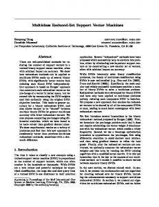
Figure 4. The fitting of a piecewise constant function.

exp(F1,1 (x)) ; p1 (2, 3|x) = 1−p1 (1|x). p1 (1|x) = P3 j=1 exp(F1,j (x)) (11) For the second layer, we compute

Equation (7) now becomes fmj = arg min

r,c,w,h,t

N X

wij |zij − f (xi ; r, c, w, h, t)|2 . (9)

i=1

For a given configuration (r, c, w, h, t), the optimal values of a are computed as ak =

PN

i=1 wij zij [(g ⊗ xi ) ∈ Rk ] . PN i=1 wij [(g ⊗ xi ) ∈ Rk ]

exp(F2,2 (x)) ; p2 (3|x) = 1 − p2 (2|x). p2 (2|x) = P3 j=2 exp(F2,j (x)) (12) Finally, the overall posterior probabilities are p(1|x) = p1 (1|x); p(2|x) = p1 (2, 3|x)p2 (2|x);

(10)

Figure 4 illustrate fitting the piecewise constant function to a set of unweighted data points. In the step (∆) in Figure 2, the most relevant feature with the smallest error is singled out to maximally reduce the classification error. In the literature, simple binary regression stumps are used [17, 15]. However, it is easy to show that the piecewise constant function combines multiple binary regression stumps, therefore enhancing the modeling capability of the weak learners and consequently improving training speed.

4. Extensions In this section, we address two useful extensions of the multiclass boosting algorithm. In the first extension, we show how to learn a tree structure which offers efficiency in both training and testing. In the second extension, we propose to train a cascade structure to deal with the vexing background class that has voluminous examples.

(13)

p(3|x) = p1 (2, 3|x)p2 (3|x). (14) P3 It is easy to verify that j=1 (j|x) = 1. Generalizing the above 3-class example to an arbitrary multiclass problem is easy. The main idea is to repeat a ‘divide-and-merge’ strategy. For a merged class, we learn a multiclass classifier to divide them. After the classifier is learned, we separate those ‘easy’ classes from the remaining classes that are merged into one class. Similarly, the posterior calculation can be carried out. The proposed tree structure is very different from the multiclass PBT algorithm [16]. First, when ‘dividing’ at each tree node, the PBT first converts a multiclass task to a binary one based on an optimal feature and then invokes boosting to learn a binary classifier; whereas we never perform such a conversion and always learn a truly multiclass classifier. Second, there is no ‘merging’ operation in the PBT. The samples are always divided till there is no further ambiguity, leading to a risk of overfitting. Since we operate at a class level (rather than a sample level as in the PBT), we seldom overfit.

4.1. Tree structure Empirical evidence tells that often, in the midst of boosting a multiclass classifier, one class (or several classes) has been completely separated from the remaining ones and further boosting yields no additional improvement in terms of the classification accuracy. This fact can be utilized for efficient training. To this end, we propose to train a tree structure.

4.2. Cascade structure The cascade structure that corresponds to a degenerate decision tree is introduced to perform learning under a rare event scenario. Such a scenario presents an unbalanced nature of data samples. The background class has voluminous samples because all data points not belonging to the object classes belong to it.

The use of cascade during online detection of object is illustrated as follows. Given an image, we want to find the instances of the interested objects in it. This is achieved via an exhaustive scanning of the image. A window W that defines a region of interest slides in the space of (x, y, θ, s), where (x, y), θ, and s are the center, orientation, and scale of the window, respectively. Only the windows that pass all stages of the cascade are subject to final classification. Denote the set of all these windows by W: Figure 5. The tree structure of a boosted multiclass classifier. (n)

(n)

W = {W |p0 (W ) < max pj (W ); n = 1, ..., Ncas }. j=1,...,J

Figure 6. The cascade of boosted multiclass classifiers.

To effectively examine more background examples, only those background examples that pass the early stages of the cascade are used for training the current stage. This is the same to the idea of negative bootstrapping in the neural network literature. However, the learned strong classifier for each stage has to be adjusted in order to reach a desired detection rate. In [17], this is done by changing the strong classifier threshold. We follow [17] to train a cascade of boosted multiclass classifiers as shown in Figure 6. The examples for the background class fed to the first stage are randomly cropped. To train a cascade of boosted multiclass classifiers, we must make sure that the training examples for class {C1 , C2 , . . . , CJ } can succeed the available stages. To achieve this, we decide to change the response function Fj (x). One simple solution is to add a constant shift T0 to the output function of the background class, F0 (x). The value of T0 is chosen to guarantee the desired detection rate. Note that here the concept of the detection rate is applied to all classes except the background class. Suppose that the desired rate is 1−α, we choose T0 such that [i]

[i]

Fi (x) ≥ F0 (x) + T0 ; x ∈ Si = {x1 , x2 , . . . , x[i] ni } (15) PJ must be valid for ⌊( j=1 nj ) ∗ (1 − α) + 0.5⌋ times. In other words, T0 is the α percentile of the values {Fj′ (x) = Fj (x) − F0 (x); x ∈ Sj , j = 1, 2, . . . , J}. It should be emphasized that the tree and cascade structures are two different concepts. The tree structure is a multiclass classifier, while the cascades consists of several stages of multiclass classifiers. In practice, the two structures can be combined to achieve better efficiency.

(16) (n) where pj is the posterior probability of W being class j when the boosted multiclass classifier for the nth cascade is used and Ncas is the number of stages in the cascade. In the case when multiple objects present in the scene, we can simply classify each window in the above set, assign it a class label and post-process those windows with severe overlapping. In the case when only one final decision is needed, such as cardiac view classification, ad hoc fusion strategies such as majority voting can be used.

5. Echocardiographic view classification In this section, we present details of our automatic system of echocardiographic view classification (EVC), where an echocardiographic video in a DICOM format is classified into three classes, namely the A4C and A2C view along with the background class, using the learned cascade of multiclass strong classifiers. The reason why we chose A2C and A4C views for our experiments is that these two views are commonly used for clinical purpose, and they are very similar to each other and hard to discriminate. Therefore, it is enough to show a proof of concept. In the future, we plan to add more views and use the same procedure for classification. The EVC system takes an echo video as input but infers the view label based on an image classification approach without considering temporal information to reduce computation time toward a real-time requirement. Only the end-diastolic (ED) frame is used for classification. The ED frame is characterized by the fact that the heart is mostly dilated. Also, the ED frame index is directly coded in the DICOM header. The overview of the EVC system is depicted in Figure 7. It consists of three modules: 1) training data collection, 2) multiclass boosting training, and 3) online view classification. During online classification, the system only analyzes the ED frame given an echocardiographic video sequence, and classifies the ED frame into one of the trained views by combining the results of all scanned subwindows. The classification result of the ED frame represents the final view of the echocardiographic video sequence.

A2C A4C

A2C 31/34=91.2% 3/48=6.2%

A4C 3/34=8.8% 43/48=89.6%

Missed 0/34=0% 2/48=4.2%

Table 1. Detection and Classification results for the test data

cates the magnitude of a high frequency of the local region. We can generate a very large number of filters by varying the type, location, and size of the filter. We trained a cascade of two multiclass classifiers, following the principles presented in section 3 and 4. For each stage of the cascade, we further trained a tree structure (as in 4.1) if applicable. To train the first cascade, we randomly selected negative samples twice more than the positives. To train the second cascade, we followed the bootstrapping procedure in section 4.2.

Figure 7. The overview of the EVC system

5.3. View classification and results (a)

(b)

(c)

(d)

Figure 8. Procedure of template image cropping. (a) A4C ED frame. (b) LV contour and bounding box. (c) Template bounding box along with LV bounding box. (d) Cropped template image.

5.1. Training data collection We used 391 A2C sequences and 466 A4C sequences for collecting training data. We first designed template layouts for the two views, which highlight their characteristic structures. The template is designed based on the left ventricle (LV) orientation and size. Specifically, for the A4C view, the template contains all four chambers; while for the A2C view, the template contains all two chambers. We manually annotated the LV endocardium to align the data and reduce the appearance variation. Given a training video sequence and its LV annotation, a template image is cropped according to the template layout and rescaled to a canonical size. The template cropping procedure is shown in Figure 8. Given a video sequence, training images are collected from five frames, i.e., the ED − 2 frame to ED + 2 frame Further, we collected additional positives by perturbing the template bounding box by a small amount around its center and in its width, height, and angle. Negative training images are collected outside the perturbing range for positives.

5.2. Multiclass boosting training We employed Haar-like local rectangle features used in [12, 17]. The Haar-like local rectangle filters provide local high frequency components in various directions and resolutions. Figure 3 shows five types of the filters we used, where the output of the filters is a scalar value by subtracting the sum of the intensity values in the white rectangle(s) from that of the grey rectangle(s). The output value indi-

We used 34 A2C sequences and 48 A4C sequences for experiments of detection and classification of cardiac view. Given a sequence, we performed exhaustive search from the left-top corner to the right-bottom corner by changing the width, height, and angle. This exhaustive search approach may yield multiple results of detections and classifications, especially around the correct view location. We employed a multiple hypotheses fusion approach based on majority voting. If the EVC system yields multiple hypotheses (classification results), the number of classification results of each view is computed and the final view is determined according to the maximum number of view classification results. If the numbers are the same, we employed a simple tie-break rule based on the mean of all the posterior probabilities the classifier provides. The detection and classification results are shown in Table 1. There are 31 out of 34 A2C sequences correctly classified and 3 sequences misclassified as A4C. In the case of A4C, there are 43 out of 48 sequences detected and classified correctly, 3 sequences misclassified as A2C, and 2 sequences failed in classification as any of the two views. Figure 9 illustrates some of the misclassified examples. As shown in the figure, these misclassified ones are very challenging even for human to discriminate. In terms of speed, on average, our system runs almost in real time at a PC with a 2GHz CPU and a 2GB memory, consuming about 1.5s to classify a sequence which typically contains a full cardiac cycle with about 30 frames.

5.4. Discussion To the best of our knowledge, the only relevant work that attempted to recognize the cardiac views is [2] where the constellation model of the cavities is used. The authors of [2] used the gray-level symmetric axis transform [14] to detect a cardiac chamber, assuming that there exists a distinct

(a) Three A2C examples misclassified to A4C

ties such as the tree structure for efficient training, the cascade training to deal with rare event detection, and always sharing local feature across the classifier outputs. In future, we plan to (i) increase the number of views in the EVC system and (ii) evaluate the proposed multiclass boosting method to detect generic objects.

References

(b) Three A4C examples misclassified to A2C Figure 9. Misclassified examples

cavity in the image for each chamber of the heart. While this assumption in general holds for the A4C view, it is invalid for the A2C view. After the chambers are detected, they modeled the constellation of the parts using the Markov random field to capture both appearances and spatial relationships of the chambers. The support vector machine classifier (SVM) is used for view classification, based on the energy vector extracted from the Markov model. Our approach is very different from [2]. While a threestage approach is presented in [2], we proposed a oneshot solution built on the machine learning and appearancebased object detection literature. One main drawback of [2] is that its performance heavily depends on the chamber detector, which has no guarantee of localizing the parts correctly. Our approach, instead, explicitly encodes the part structure into template design and searches the desired part structure in running time. In fact, one byproduct of our approach is accurate localization of the chambers. In experiments, a small database was used in [2], with 15 echo videos of normal cases and six videos of abnormal cases. Four experimental settings were evaluated and accuracies ranging from 54% to 88% were reported using the leave-one-out scheme. It is hard to predict how their performance scales to a large database. We used a large database: training uses 391 A2C and 466 A4C videos and testing uses 34 A2C and 48 A4C sequences. We achieved an overall accuracy of 90.2%. Also there is no computational speed reported in [2]; while we run almost in real time. Presumably, computation in [2] cannot be close to real time because fitting a Markov random field model is slow.

6. Conclusions We proposed a multiclass boosting procedure for simultaneous detection of multiple objects and successfully applied it to automatic view classification of echocardiographic sequences. The image-based multiclass boosting is a one-shot solution that possesses many promising proper-

[1] T. Dietterich and G. Bakiri. Solving multiclass learning problem via error-correcting output codes. Journal of Artificial Intelligence, 2:263–286, 1995. [2] S. Ebadollahi, S. Chang, and H. Wu. Automatic view recognition inechocardiogram videos using parts-based representation. In CVPR, pages 2–9, 2004. [3] Y. Freund and R. Schapire. A decision-theoretic generalization of online leaning and an application to boosting. Journal of Computer and System Sciences, 5(1):119. [4] J. Friedman, T. Hastie, and R. Tibshirani. Additive logistic regression: a statistical view of boosting. Ann. Statist., 28(2):337–407, 2000. [5] T. Hastie, R. Tibshirani, and J. Friedman. The Elements of Statistical Learning. Springer, 2001. [6] S. Krempp, D. Geman, and Y. Amit. Sequential learning of reusable parts for object detection. Technical report, CS Johns Hopkins Univ., 2002. [7] S. Lazebnik, C. Schmid, and J. Ponce. Affine-invariant local descriptors and neighborhood statistics for texture recognition. In ICCV, 2003. [8] Y. LeCun, F. Huang, and L. Bottou. Learning methods for generic object recognition with invariance to pose and lighting. In CVPR, 2004. [9] F. Li, R. Fergus, and P. Perona. A bayesian approach to unsupervised one-shot learning of object categories. In ICCV, 2003. [10] S. Li and Z. Zhang. Floatboosting learning and statistical face detection. PAMI, 26(9), 2004. [11] D. Lowe. Object recognition from local scale-invariant features. In ICCV, 1999. [12] C. Papageorgiou, M. Oren, and T. Poggio. A general framework for object detection. In ICCV, 1998. [13] R. Schapire and Y. Singer. Improved boosting using confidence-rated predictions. Machine Learning, 37(3):297– 336, 1999. [14] H. Tagare, F. Vos, C. Jaffe, and J. Duncan. Arrangement : A spatial relation between parts fo evaluating similarity of tomograhic section. PAMI, 17:880–893, 1995. [15] A. Torralba, K. Murphy, and W. Freeman. Sharing features: efficient boosting procedures for multiclass object detection. In CVPR, 2004. [16] Z. Tu. Probabilistic boosting-tree: Learning discriminative models for classification, recognition, and clustering. In ICCV, 2005. [17] P. Viola and M. Jones. Rapid object detection using a boosted cascade of simple features. In CVPR, pages 511–518, 2001.