Using McMillan's ordering algorithm [25] they are guaranteed to project scene samples onto the new ..... William R. Mark, Leonard McMillan, and Gary Bishop.
Image-Based Rendering for Non-Diffuse Synthetic Scenes Dani Lischinski
Ari Rappoport
The Hebrew University
Abstract. Most current image-based rendering methods operate under the assumption that all of the visible surfaces in the scene are opaque ideal diffuse (Lambertian) reflectors. This paper is concerned with image-based rendering of non-diffuse synthetic scenes. We introduce a new family of image-based scene representations and describe corresponding image-based rendering algorithms that are capable of handling general synthetic scenes containing not only diffuse reflectors, but also specular and glossy objects. Our image-based representation is based on layered depth images. It represents simultaneously and separately both view-independent scene information and view-dependent appearance information. The view-dependent information may be either extracted directly from our data-structures, or evaluated procedurally using an image-based analogue of ray tracing. We describe image-based rendering algorithms that recombine the two components together in a manner that produces a good approximation to the correct image from any viewing position. In addition to extending image-based rendering to non-diffuse synthetic scenes, our paper has an important methodological contribution: it places image-based rendering, light field rendering, and volume graphics in a common framework of discrete raster-based scene representations.
1 Introduction Image-based rendering is a new rendering paradigm that uses pre-rendered or preacquired reference images of a 3D scene in order to synthesize novel views of the scene. This paradigm possesses several important advantages compared to traditional rendering: (i) image-based rendering is relatively inexpensive and does not require special purpose graphics hardware; (ii) The rendering time is independent of the geometrical and physical complexity of the scene being rendered; and (iii) The pre-acquired images can be of real scenes, thus obviating the need to create a full geometric 3D model in order to synthesize new images. While the ability to handle real scenes has been an important motivating factor in the emergence of image-based rendering (particularly in the computer vision community [17]), it soon became clear that image-based rendering is also extremely useful for efficient rendering of complex synthetic 3D scenes [5, 12, 22, 23, 29]. Unfortunately, most current imagebased rendering methods operate under the assumption that all of the visible surfaces in the scene are opaque ideal diffuse (Lambertian) reflectors, i.e., it is assumed that every point in the scene appears to have the same color when viewed from different directions. However, in practice, both real and synthetic scenes often contain various non-diffuse surfaces, such as specularly reflecting Fig. 1. The result of warping two different refmirrors, shiny floors, glossy tabletops, erence views of a scene to a common new view. etc. If any of these non-diffuse surfaces The mirror reflections in the box are incorrect are visible in the reference images of the and inconsistent.
scene, new images of the scene produced by most current image-based rendering methods will be incorrect, exhibiting potentially severe inconsistencies, as illustrated in Figure 1. The inability of image-based rendering techniques to handle non-diffuse scenes correctly, is a major limitation of their usefulness, applicability, and power. It should be noted here that one particular variety of image-based rendering, referred to as light field rendering [11, 20] is not subject to the above limitation, but at a significant storage penalty. The main contribution of this paper is a new image-based rendering approach that correctly handles non-diffuse synthetic scenes with general view-dependent shading phenomena, such as specular highlights, ideal specular reflections, and glossy reflections. In our approach, a scene is represented as a collection of parallel projections with multiple depth layers (LDIs) [12, 23]. All view-independent scene information (i.e., geometry and diffuse shading) is represented using three orthogonal high-resolution LDIs. The view-dependent scene information is represented as a separate (larger) collection of low-resolution LDIs. Each of these LDIs captures the appearance of the scene from a particular direction. We describe image-based rendering algorithms that recombine these two components together to quickly produce a good approximation to the correct image of the scene from any viewing position. By separating the representation in the manner outlined above, we are able to obtain results superior in quality to those produced by light field rendering methods, while requiring considerably less storage. Our image-based rendering techniques produce images with view-dependent shading and reflections whose quality is comparable to those generated by a conventional ray tracer, but faster. Another important contribution of this paper is a methodological one. Our approach places image-based rendering, light field rendering, and volume graphics [13] in a common framework: the framework of discrete raster-based scene representations. This common framework enables better understanding of the relative advantages and disadvantages of these techniques.
2 Related work An image-based rendering technique can be thought of as a combination of a discrete raster-based scene representation with a rendering algorithm that operates on this representation to produce images from various views. The rendering algorithm typically utilizes the regularity, uniformity, and the bounded size of the raster-based representation to produce the new views rapidly. Four main kinds of raster-based representations have been previously explored: image-based representations, discrete 4D light fields, discrete volumetric representations, and ray representations. 2.1 Image-based representations Image-based rendering techniques typically represent a scene as a collection of reference images: scene projections sampled on a discrete grid. This projections can be spherical, cylindrical [4, 26], or planar [5, 17, 22, 28]. Each projection pixel can be thought of as a scene sample, because it represents the color (and sometimes the depth) of the nearest point in the scene that can be seen along the corresponding projection line. New images can be generated from one or more projections by warping these scene samples to the desired view. In order to correctly warp a scene sample, we must know its depth. Depth information is either encoded implicitly in the form of correspondences between pairs of points in different projections [17, 26], or it can be stored
explicitly with each scene sample. For example, in the case of synthetic scenes depth information is readily available. In addition to obtaining depths or correspondences, the key challenge in these approaches is to handle the gaps that appear in the synthesized images. Such gaps appear when areas in the reference images are stretched by the warp to the new image, and when parts that are occluded in all of the reference images come into view. Mark et al. [22] handle these problems using multiple reference images, each represented as a mesh of micro-polygons. Gortler et al. [12] use a layered depth image (LDI) and “splat” each pixel onto the screen [32]. Layered depth images were also used by Max [23, 24] in order to represent in a hierarchical fashion and render complex photorealistic models of botanical trees. There are similarities between his approach and the one presented in this paper: both approaches use parallel projection LDIs, and store a normal with each scene sample in order to perform shading after the reprojection. However, our approach concentrates on the issue of handling view-dependent shading phenomena, which was not addressed by Max. As pointed out earlier, creating a new image by warping scene samples is only correct when the samples correspond to ideal diffuse surfaces. There have been a few attempts to extend reprojections and view-interpolation to non-diffuse scenes [1, 2, 6], but these approaches are not completely image-based. They require access to the original scene geometry to handle various cases in which reprojection cannot produce the correct results. Thus, these methods handle diffuse pixels quickly, but still have to do a lot of work for the remaining pixels. 2.2 Light field rendering While image-based rendering techniques represent both the geometry and the color of each scene sample, light field rendering techniques [11, 20] avoid the representation of geometry altogether. Instead they represent a scene as a 4D subset of the complete 5D light field that describes the flow of light at all positions in all directions. This 4D function, which Gortler et al. dub a Lumigraph, describes all of the light entering or leaving a bounded region of space. Once the Lumigraph has been constructed, images of the region’s contents can be quickly generated from any viewpoint outside the region. Light field rendering is simpler and more robust than most previous image-based rendering techniques because it does not require depth values, optical flow information, or pixel correspondences, and it is not limited to diffuse scenes. However, it also has several significant limitations: (i) high-fidelity light fields require a very large amount of storage; (ii) computing the light field of a synthetic scene can take a very long time; and (iii) the 4D light field describes the flow of light in a bounded region of space free of objects, and it is not yet clear how to extend light-fields to allow free navigation inside a scene. 2.3 Volume graphics Image-based rendering techniques were not the first to utilize the advantages of regular and uniform discrete representation of 3D scenes: similar representations have been actively explored in the field of volume visualization [9, 15, 16, 18, 32]. In particular, a subfield of volume visualization, referred to as volume graphics [13] is concerned with the synthesis, representation, manipulation, and rendering of volumetric objects stored in a 3D volume buffer. Unlike volume visualization, which focuses primarily on sampled and computed volumetric datasets, volume graphics is concerned primarily with volumetric representation of synthetic 3D scenes. Similarly
to image-based rendering, volume graphics is insensitive to the geometric complexity of the scene and of the objects contained in it. Volumes have an advantage over images in that they constitute a more complete representation of the environment: not only the boundary of the objects is represented, but also their interior. However, the price of the extra dimension is much higher storage requirements and longer rendering times. Several researchers in volume graphics have investigated algorithms for rendering non-diffuse synthetic scenes from their volumetric representation. Volumetric ray tracing [19, 31] can be used for this purpose, handling specular reflections and other nondiffuse phenomena via recursive tracing of secondary rays. Yagel et al. [33] describe discrete ray tracing, a technique in which discrete (voxelized) rays are tracked through the 3D volume buffer until they encounter a voxel occupied by a voxelized surface. Our proposed approach utilizes a related technique, which traces a ray in a layered depth projection of the scene. The discrete scene representation and the rendering algorithms that we propose to explore can be viewed as bridging the gaps between the image-based rendering, light field rendering, and volume graphics approaches surveyed above. 2.4 Ray representations Researchers in solid modeling have explored object representation schemes based on ray sampling. Van Hook [30] extended the ordinary z-buffer by storing a list of objects at each pixel, supporting faster visualization of Boolean operations for simulation of NC machining operations. This method requires special purpose hardware that is not currently available. Groups from Cornell and Duke universities have devised a hardware architecture called the “ray casting engine”, in which a geometric object is represented by a discrete 2D matrix defined by a parallel projection of the surfaces defining the object in a certain direction. Each matrix element contains a list of surfaces pierced by the corresponding ray. The resulting representation was dubbed the “ray representation” or “rayrep” [10]. It was argued that using the rayrep, several important solid modeling operations are easier to solve [27]. One of these operations was ray tracing the solid, but the results were not of high visual quality. Recently, Benouamer [3] proposed using three sets of rayreps projected in orthogonal directions for computing Boolean operations when converting CSG objects to a boundary representation (Brep). The rayreps are generated by ray casting, and the Brep is obtained by a surface reconstruction algorithm in the spirit of the “marching cubes” algorithm [21]. The emphasis in his work is on the resulting geometry, its tolerance with respect to manufacturing applications, and the simplicity of implementation rather than on rendering and visual quality.
3 A new discrete representation The main new idea behind our approach is to represent simultaneously but separately both view-independent scene information (geometry, diffuse shading, etc.) and viewdependent appearance information. The two components are combined during rendering to efficiently produce correct images of non-diffuse scenes. Both kinds of scene information are represented using a collection of parallel projections of the scene, where each projection is a layered depth image (LDI) [12, 23] 1 . 1 The
LDIs described by Gortler et al. [12] are defined using a general perspective projection of the scene.
h d
c
g f
b
e
a 1 2 3 4 5 6 7 8 9 10 11 12 (a)
(b)
(c)
Fig. 2. (a) A parallel LDI of a simple 2D scene. Pixel 6 in the LDI stores scene samples a b c d, and pixel 9 stores scene samples e f g h. (b) and (c) illustrate (in 2D) the view-independent LDIs and the LLF, respectively.
Each LDI pixel contains a list of scene samples corresponding to all surface points in the scene intersected by the projection ray through the center of the pixel (see Figure 2a). The scene samples all lie on a 2D raster, when seen from the direction of projection, but their positions along the projection axis can be arbitrary (thus, there is no discretization along the depth axis). The difference between the representation of the view-independent and the view-dependent components is in the type of information stored with each scene sample and in the number of projections. 3.1 The layered depth cube The view-independent component of our representation consists of three high-resolution parallel LDIs corresponding to three orthogonal directions (see Figure 2b). We refer to this component as the layered depth cube (LDC). With each scene sample of the LDC we store its depth value (the orthogonal distance from a reference plane perpendicular to the direction of projection). We also store the surface normal, the diffuse shading, a bitmask describing the visibility of the light sources, and the directional BRDF at the surface point2 . Note that for diffuse scenes this representation is complete (modulo the finite spatial resolution of the LDIs). Specifically, if h is the spacing between adjacent pixels in the LDIs, p we are guaranteed to have at least one scene sample on any surface element of size 3 h, regardless of its orientation. 3.2 The layered light field The view-dependent component of our representation is referred to as the layered light field (LLF). The LLF consists of a potentially large collection of low-resolution parallel LDIs corresponding to various directions (we have experimented with 66, 258, and 1026 directions, uniformly distributed on the unit sphere), as illustrated in Figure 2c. Each scene sample in the LLF contains, in addition to its depth, the total radiance leaving the scene sample in the direction of projection. Thus, each of the LDIs samples Similarly to Max [23], we use parallel projections since they offer computational advantages, as we shall see in section 4.3. 2 In practice, we store an index into a table containing the material properties of surfaces in the scene.
the light field along oriented lines parallel to the direction of projection. Assume that the LLF has n LDIs, each with spacing of h between adjacent pixels.pIn this case, we are guaranteed that any point p in the scene lies within a distance of 22 h from n light field samples, each corresponding to a different direction. Thus, given any point p in the scene we can reconstruct the light field at that point by interpolating between n samples. Naturally, the accuracy of the reconstruction depends on the number of directions n and on the spacing h between adjacent parallel projection lines. 3.3 Rendering overview At this point, we have the necessary ingredients for describing our non-diffuse imagebased rendering algorithm for synthetic scenes. Rendering proceeds in two stages: First, we apply 3D warping to the high-resolution view-independent LDIs. This stage is described in more detail in Section 4.1. The 3D warping results in a primary image, which is a correct representation of the geometry of the scene, as seen from the new viewpoint, along with the diffuse component of the shading. In each pixel of the primary image we store the scene sample visible through that pixel. The second stage utilizes the normal, the light source visibility mask, and the directional BRDF at each visible scene sample to compute the view-dependent component of the shading. First, specular highlights from the light sources in the scene are added, by simply evaluating the local specular shading model (e.g., Phong) for each of the visible light sources (visibility is stored in the light source bitmask). Then, to add reflections of other objects in the scene we use two techniques: 1. Light-field gather: this technique integrates the light field at the point of interest using the directional BRDF to weigh each incoming direction. The light field is reconstructed from the LLF as described in Section 4.2. Light-field gather works very well with glossy objects with fuzzy reflections, but in order to generate sharp reflections (e.g., on mirrors) it is more effective to use image-based ray tracing. 2. Image-based ray tracing: this technique recursively traces reflected rays from the point of interest. These rays are traced using the view-independent LDIs, as described in Section 4.3. After k reflections recursion is terminated and we perform a light-field gather. Experiments have shown that deeper recursion increases the rendering time, but allows us to use a sparser LLF. In most scenes, tracing just one generation of reflected rays yields very good results. 3.4 Discussion Our scene representation can be thought of as a parametric family of image-based scene representations. Different members of this family are obtained by different choices of the number of the directions in the LLF, the spatial resolution of the different types of LDIs, and the depth of recursive ray tracing. In particular, it is shown below that within this family we can obtain an image-based representation that is essentially a slightly generalized version of the discrete 4D light field [11, 20]. Another member of the family is an efficient alternative to the 3D volume buffer [13]. Comparison with light field rendering. If the light-field LDIs are of sufficiently high resolution, and if their corresponding directions sample the unit sphere densely enough, we obtain a discrete representation of the light field, similar to the 4D discrete light fields used in light field rendering [11, 20]. Recall that these 4D light fields require the viewpoint to lie in a free region of space, outside the region represented by the light
field. The LLF removes this restriction by storing multiple layers per pixel, and by storing a depth value along with each scene sample. The 4D light field stores only information describing the appearance of the scene from different directions, but it does not contain any explicit geometric information beyond that. This allows images of the scene to be rendered very simply and rapidly, but requires high directional and spatial resolutions to achieve high image quality, resulting in potentially enormous storage requirements. Gortler et al. [11] observe that by using approximate geometric information the quality of the reconstruction can be significantly improved. Our representation takes this idea even further: it relies on the LDC to accurately represent the scene geometry, and uses the LLF only to supplement the view-dependent shading where needed. Thus, we obtain high quality images using low directional and spatial resolution of the light field. The price we must pay for these advantages is somewhat slower rendering: a classical case of space-time trade-off. Comparison with volume graphics. Our view-independent representation component resembles volumetric representations of synthetic scenes [13]. Indeed, the similarity between a projection-based representation and a volumetric one is not at all surprising, since it is easy to see how a volumetric representation can be constructed from the projection-based one (for example, such techniques are used in medical imaging for constructing volume data from CT scans). However, with the aid of 3D image warping, we can produce images of the scene directly from our projection-based representation, without ever constructing the full 3D volume buffer. The main differences between our representation and a full 3D volume buffer are: 1. Three n n LDIs require less storage than a volume buffer of the same resolution, as long as the average number of depth layers per pixel is less than n=3. It seems reasonable to assume that for high-resolution discrete representations, the spatial resolution of the scene projections is considerably higher than the average depth complexity (i.e., a 5122 LDI is likely to have average depth complexity much lower than 512=3). Thus, the LDIs should be much more economical in terms of storage than a full 3D volume buffer, particularly at high resolutions. 2. The LDIs have infinite resolution along the projection axis of each LDI, whereas a volume buffer is not capable of resolving cases where two or more surfaces occupy the same voxel. 3. Similarly to image-based ray tracing, it is possible to render images of non-diffuse scenes by recursively tracing discrete rays in the 3D volume buffer [33]. In our representation, the LLF lets us eliminate the recursion altogether, or terminate it after a small number of reflections.
4 Computational elements for rendering 4.1 3D warping Rendering begins by 3D warping the view-independent LDIs in order to generate a primary image of the scene. This stage determines which scene sample is visible at each pixel of the new image. We have implemented the fast LDI warping algorithm described by Gortler et al. [12]. There are, however, a few important differences between our implementation and theirs. Gortler et al. warp a single LDI to produce a new image. Using McMillan’s ordering algorithm [25] they are guaranteed to project scene samples onto the new image plane in back-to-front order. Thus, there is no need to perform depth comparisons, and splatting can be used to fix holes due to stretching of the scene
samples. In our case, all three LDIs must be warped to ensure that no surfaces are missed (since there might be surfaces in the scene that are only sampled by one of the three LDIs). Therefore, we do perform a depth comparison before writing each scene sample onto the new image. It should be noted that the cost of performing these comparisons is negligible. Also, since scene samples are not guaranteed to arrive in back-to-front order we can’t use Gortler’s simple splatting approach. Currently, in order to handle holes we first warp the LDIs, and then scan the resulting image looking for holes (pixels not covered by any scene samples and pixels whose depth is significantly larger than that of most of their neighbors). For each pixel suspected as a hole, we follow a ray from the eye to find the visible scene sample, using the image-based ray tracing algorithm of Section 4.3. In the examples shown in Section 5 there were less than two percent of such pixels. However, this problem clearly deserves a more robust solution, and we hope to address it in the future. 4.2 Light field gather Next, we need to solve the following problem: given a point p in the scene, the directional BRDF (without the diffuse component) �bd , and an outgoing direction ! ~ o, estimate the view-dependent component of the radiance reflected from p in direction ~!o . We solve this problem by using the LLF to reconstruct the light field at p and “pushing” it through the BRDF:
Lout = 0 foreach direction ! ~ i in the LLF !i � ~!o ) > 0 if �bd (~ Lin = radiance arriving at p from ~ !i !i � ~ !o ) Lin cos �i ~ !i Lout = Lout + �bd (~ endif endfor To reconstruct the radiance arriving at p from a direction in the LLF we project p onto the reference plane of the corresponding LDI, and establish the coordinates of the four nearest LDI pixels. At each of these pixels, we scan the list of scene samples until we find one visible from p (i.e., with depth greater than that of p), and retrieve the radiance stored in this sample. The requested radiance value is then obtained by bilinear interpolation of the four retrieved values. The above routine works well for glossy surfaces, but is not well-defined for ideal specular reflectors, because their BRDF is only non-zero in the mirror-reflected direction. In this case, we find all of the directions in the LLF that fall within a small cone !i (the mirror-reflected direction). The opening angle of the cone depends on around ~ the directional density of the LLF: it is chosen large enough so that at least three directions would be found. Radiance values are retrieved from each of these directions as above and the radiance arriving at p from ~ ! i is estimated by a normalized weighted average of these values. The weight for each LLF direction is cos n �, where � is the !i , and n is a user-specified parameter. angle between the LLF direction and ~ 4.3 Image-based ray tracing For the sake of exposition, we begin by describing a rather naive algorithm, which will then be improved. Given a 3D ray and a parallel LDI, we first project the ray onto the reference plane of the LDI, and clip the resulting 2D ray to the square window
containing the projection of the scene. We then visit all of the pixels in the LDI that are crossed by the 2D ray, starting from the origin. As we step from one pixel to the next, we keep track of the depth interval Z in � Zout ] spanned by the 3D ray while inside each pixel. The depths of the scene samples in each visited pixel are compared against this interval. If a single sample is found whose depth lies inside Zin ; �� Zout + �], we report this sample as a ray-surface intersection. If more than one depth value falls inside the depth interval, we report the value nearest to the ray’s origin. The magnitude of � depends on the resolution of the LDI and on the angle between the surface normal of the scene sample and the direction of projection. This operation must be performed for each of the three LDIs, because there might be surfaces that are only sampled by one of the LDIs, being parallel to the projection directions of the other two. The problem with the simple routine described above is that it may have to visit up to 6n LDI pixels (at most 2n pixels in each of the three n n LDIs). At each LDI pixel, it does O(d) work, where d is the depth complexity there. As a result, this algorithm is too slow to be used with high-resolution LDIs. Fortunately, the algorithm can be sped up drastically by using hierarchical data structures. Consider the case of an LDI with a single depth layer — a regular range image. To speed up image-based ray tracing we construct a quadtree for this range image. An internal node in the quadtree stores the minimum and the maximum depth of all the pixels in the corresponding sub-region of the range image. A leaf node stores the depth of a single pixel. Given a 2D ray we can establish whether an intersection exists by a simple depth-first traversal of the quadtree. Whenever we encounter an internal node whose depth range is disjoint from the depth interval of the ray, the entire subtree can be safely skipped. If the depth intervals are not disjoint, we recursively traverse the node’s children, visiting them in the same order as the ray. This algorithm is similar to one described by Cohen and Shaked [7] for speeding up ray tracing of terrain. This similarity is not surprising, since digital terrain data is a height field, just like a range image. To extend the above algorithm to LDIs with multiple layers, think of an LDI as a stack of range images: The topmost layer is the “normal” image of the scene, after parallel projection and hidden surface removal. The second layer is an image showing only those parts of the scene occluded by exactly one surface, and so forth. We could simply construct a quadtree for each range image in the stack, and have each ray traverse each of these quadtrees independently. However, we can perform the traversal in a more efficient manner by taking advantage of the special structure possessed by successive depth layers of the same LDI. Note that a pixel in depth layer i + 1 is non-empty (contains a scene sample) only if the same pixel was non-empty in layers 1 through i. This means that if we encounter an empty node in the quadtree of layer i, Traverse(node, ray, Z in , Zout ): there is no need to traverse the cor- if Zout < node:Zmin return responding nodes in layers i + 1 and if Zin > node:Zmax then Traverse(node.crosslink, ray, Z in , Zout ) deeper. Thus, we begin by constructing return a separate quadtree for each depth layer of the LDI, but then we create cross links endif between the quadtrees: each non-empty if Leaf(node) then scan layers for intersections node in the quadtree of layer i points to its twin in the quadtree of layer i + 1. else foreach non-empty child of node Update Zin and Zout Now, given a ray, we start a recursive Traverse(child, ray, Zin , Zout ) traversal from the root node of the first endfor layer’s quadtree. The traversal routine is given in the pseudocode on the right. As endif
Table 1. Scene statistics and rendering times. All sizes are in megabytes, all timings are in seconds on a 200 MHz Pentium-Pro running Linux.
# primitives LDC size avg (max) # layers LLF resolution LLF size construction time warping time view-dependent pass 0 / 1 / 7 reflections total rendering time Rayshade time
sphere & cylinder 8 42.5 0.97 (3) 258 642 11.7 582 2.9 2.7 / 4.3 / 4.5
teapot 9,121 28.8 0.53 (4) 1026 642 19.3 726 1.3 3.2 / – / –
teapot & spheres 9,179 50.6 1.23 (10) 66 642 3.1 2420 3.5 2.7 / 11.1 / –
5.6 / 7.2 / 7.5 8.2
4.5 / – / – 126.1
6.2 / 14.6 / – 22.2
before, Zin and Zout is the depth interval spanned by the ray inside the node. Note that the non-empty children of a node should be visited in the order in which they are encountered by the ray.
5 Results In this section we demonstrate our approach on several non-diffuse test scenes. We compare the resulting images to those generated by conventional ray tracing, which is a very accurate method for computing view-dependent reflections. In all our test cases we have outperformed ray tracing in terms of computing time. The visual quality of the reflections is comparable to that achieved by ray tracing, even on ideal specular reflectors. Furthermore, for glossy surfaces with fuzzy reflections we achieve superior quality along with a dramatic speedup. We have extended Rayshade [14], a public domain ray-tracer, to generate parallel LDIs of non-diffuse synthetic 3D scenes. One version of the resulting program is used to generate the LDC, while another version computes the LLF. Our current implementation inserts into a particular LDI only scene samples that are front facing with respect to the parallel projection directions. Thus, the LDC actually consists of six LDIs (two for each of the three orthogonal axes), and not three LDIs as described earlier. We expect that using only three LDIs, each containing both front- and back-facing scene samples, would prove more economical both in terms of storage and in terms of processing times. We have experimented with three test scenes. Various scene statistics and rendering times are summarized in Table 1. Our first test scene contains a sphere and a cylinder with a mirror-like surface inside a box with diffuse walls and glossy (but not reflective) floor. The scene is illuminated from above by four point light sources. The average depth complexity for this scene is 0.97 (it is less than 1, because the box containing the scene is missing one wall and has no ceiling). The storage requirements for both components of our representation are 54.2 megabytes. Note that this statistic is the raw size of our non-optimized data structures. For example, we currently store the normal as three floating point numbers, whereas a more efficient implementation could have used two fixed point numbers,
in addition to some form of geometric compression [8]. Still, note that these storage requirements are considerably lower than those of a 512 3 3D volume buffer, which would have required 128 megabytes, even if only one byte per voxel was used. A 32 32 2562 Lumigraph data structure requires 192 megabytes of raw storage, and would have taken about 8,400 seconds to compute for this scene, while our representation was constructed in less 582 seconds. Furthermore, recall that six such Lumigraph slabs are required to cover all viewing directions. Figure 3 shows four 256 256 images of the same scene from an arbitrarily chosen viewpoint. Image (d) was rendered using Rayshade, while the other three were generated using our (precomputed) image-based representation. In all three images the six view-independent LDIs were first warped to produce a primary image without reflections, which were then added using three different techniques. In (a) view-dependent reflections were computed by performing a light-field gather (Section 4.2) at each reflective pixel, using a specular exponent n = 40. In (b), reflections were added by tracing one generation of reflected rays using the image-based ray tracing algorithm described in Section 4.3. In (c), reflections were added by recursive image-based ray tracing with up to seven generations of reflected rays. The LLF in all three images consists of 258 LDIs corresponding to uniformly distributed directions on the sphere. Since the directional resolution of the LLF is relatively low, when we use the light-field gather on ideal specular reflectors, the resulting reflections appear blurry (3a). Note, however, that the geometry of the scene is still sharp and accurate. This is in contrast to light field rendering techniques, where lowering the resolution of the discrete 4D light field results in overall blurring of the image. Tracing one generation of reflected rays drastically improves the accuracy of the reflections at a modest additional cost. Allowing deeper recursion further improves the recursive reflections visible in the image (the reflection of the sphere in the cylinder), and the resulting image (3c) is almost indistinguishable from the one generated by Rayshade (3d). Note that for a scene as simple as this one (eight simple primitives), ordinary ray tracing is extremely fast: in fact, it took Rayshade only 8.2 seconds to produce the image in Figure 3(d). Still, even for this simple scene, our image-based rendering algorithm outperforms Rayshade. It is interesting to examine the effect of the number of projections used in the LLF on the quality of the reflections. Figure 4 shows images that were generated using 66, 258, and 1026 directional samples in the LLF. As the directional resolution of the LLF increases, there is noticeable improvement in the accuracy of the reflections in the top row, which uses light-field gather to compute the view-dependent reflections. In the bottom row, which uses one level of image-based ray tracing, the effect is not nearly as drastic. These results illustrate that recursive image-based ray tracing effectively compensates for low directional resolution in the LLF. The case of near-ideal mirror reflectors is particularly demanding, and, as just shown, such surfaces are better handled by using at least one level of image-based ray tracing. However, for rougher glossy surfaces, an LLF with reasonable directional resolution suffices to produce a good approximation to the exact image. Figure 5 shows a teapot on a glossy floor. The left image was produced by our image-based approach, using a light field gather at each reflective pixel. The right image was produces by Rayshade. Rayshade can only generate glossy reflections by supersampling. As a result, Rayshade takes twenty-eight times longer3 than our method to generate the image, and the fuzzy reflection is still somewhat noisy. (Although, as a side-effect of the supersampling the Rayshade image is anti-aliased, while our image is not). 3 Rayshade
timing were measured using a uniform grid to accelerate ray-scene intersections.
Fig. 3. From left to right: (a) warp + light-field gather; (b) warp + one level of reflection + lightfield gather; (c) warp + seven levels of reflections; (d) Rayshade. 66 258 1026
Fig. 4. The effect of the LLF directional resolution on reflection quality. Top row: warp + light field gather; Bottom row: warp + one level of reflection + light-field gather.
Fig. 5. Glossy reflections: left (a) our method; right (b) Rayshade (using supersampling).
Fig. 6. Higher depth complexity: right (a) our method; left (b) Rayshade.
Note that for this scene, the warping stage is roughly twice as fast as in the previous scene (see Table 1). The reason is that the LDIs in the teapot scene have roughly twice lower average depth complexity (see Table 1). The time of the view-dependent pass on the other hand is somewhat higher for this scene. The main reason is that there are more directions in the LLF, and our current implementation of the light-field gather simply loops over all of these directions, rather than employing a more sophisticated search scheme. Finally, we tested our method on a scene with higher depth complexity, shown in Figure 6. The LDIs in our image-based representation of this scene have up to 10 depth layers per pixel. As expected, the total rendering time for our method is larger than for the simple scene in Figure 3: warping takes slightly longer because of increased depth complexity, and for the same reason image-based ray tracing takes longer in the viewdependent pass. Again, our approach has generated the image faster than Rayshade. The results in this section demonstrate that our technique can be considered outputsensitive with respect to view-dependent shading: For diffuse scenes, the technique is, in principle, as efficient as previous reprojection methods. We pay an extra price only in non-diffuse scenes, and the price is proportional to the number of visible non-diffuse points. Furthermore, ideal mirror reflections take longer to produce than fuzzier glossy reflections.
6 Conclusions We have introduced a new image-based representation for non-diffuse synthetic scenes, and have described efficient rendering algorithms that correctly handle view-dependent shading and reflections. Our scene representation is more space-efficient than previous discrete scene representations that support non-diffuse scenes, namely the 4D light field and the 3D volume buffer. Our results demonstrate that our approach is capable of producing view-dependent shading and reflections whose quality is comparable to that of conventional ray tracing, while outperforming ray tracing even on simple scenes. We believe that the performance gap between our technique and ray tracing will continue to grow as we further optimize and tune our implementation, and apply our techniques to more complex scenes. The main disadvantage of our approach is that the size of our data structures and consequently the rendering time depend on the depth complexity of the scene. We should investigate ways for reducing the number of layers that must be represented in our data structure without affecting the accuracy of the resulting images. There are many ways to further optimize and improve the techniques that we have described: � In order to avoid warping all of the LDIs for each frame, we should investigate the possibility of pre-warping the LDIs to a single reference LDI once in several frames, similarly to Gortler et al.[12].4 � Geometric as well as entropy compression techniques for our representation should be developed. There is currently considerable redundancy in our representation, and we should explore ways of eliminating it. � It would be useful to have an automatic way of determining a good combination of representation parameters (LDI resolutions, number and distribution of directions in the LLF) for a particular scene. Furthermore, we should explore an adaptive variant of our representation, rather than using uniform directional and spatial resolutions. 4 Thanks
to an anonymous reviewer for suggesting this idea.
� �
In order to ensure high visual accuracy of the rendered images we should investigate efficient and robust anti-aliasing techniques. This issue has not been resolved yet in the context of image-based rendering, and progress in this area could significantly contribute to other image-based rendering techniques as well. Similarly to most previous image-based representations, our representation is only effective for static scenes. A change in the scene (including motion of objects, changes in material properties, and in the positions and intensities of light sources) currently requires the entire representation to be recomputed. Efficiently updating the representation after a change in the scene is an interesting direction for future research.
Acknowledgements:. This research was supported in part by the Israel Science Foundation founded by the Israel Academy of Sciences and Humanities, and by an academic research grant from Intel Israel.
References 1. Stephen J. Adelson and Larry F. Hodges. Generating exact ray-traced animation frames by reprojection. IEEE Computer Graphics and Applications, 15(3):43–52, May 1995. 2. Sig Badt, Jr. Two algorithms taking advantage of temporal coherence in ray tracing. The Visual Computer, 4(3):123–132, September 1988. 3. M.O. Benouamer and D. Michelucci. Bridging the gap between CSG and Brep via a triple ray representation. In Proc. Fourth ACM/Siggraph Symposium on Solid Modeling and Applications, pages 68–79. ACM Press, 1997. 4. Shenchang Eric Chen. QuickTime VR — an image-based approach to virtual environment navigation. In Computer Graphics Proceedings, Annual Conference Series (Proc. SIGGRAPH ’95), pages 29–38, 1995. 5. Shenchang Eric Chen and Lance Williams. View interpolation for image synthesis. In Computer Graphics Proceedings, Annual Conference Series (Proc. SIGGRAPH ’93), pages 279–288, 1993. 6. Christine Chevrier. A view interpolation technique taking into account diffuse and specular inter-reflections. The Visual Computer, 13:330–341, 1997. 7. Daniel Cohen and Amit Shaked. Photo-realistic imaging of digital terrains. Computer Graphics Forum, 12(3):363–373, 1993. Proceedings of Eurographics ’93. 8. Michael F. Deering. Geometry compression. In Computer Graphics Proceedings, Annual Conference Series (Proc. SIGGRAPH ’95), pages 13–20. Addison Wesley, August 1995. 9. Robert A. Drebin, Loren Carpenter, and Pat Hanrahan. Volume rendering. In John Dill, editor, Computer Graphics (SIGGRAPH ’88 Proceedings), volume 22, pages 65–74, August 1988. 10. J. L. Ellis, G. Kedem, T. C. Lyerly, D. G. Thielman, R. J. Marisa, J. P. Menon, and H. B. Voelcker. The ray casting engine and ray representations: a technical summary. Internat. J. Comput. Geom. Appl., 1(4):347–380, 1991. 11. Steven J. Gortler, Radek Grzeszczuk, Richard Szeliski, and Michael F. Cohen. The Lumigraph. In Computer Graphics Proceedings, Annual Conference Series (Proc. SIGGRAPH ’96), pages 43–54, 1996. 12. Steven J. Gortler, Li-Wei He, and Michael F. Cohen. Rendering layered depth images. Technical Report MSTR-TR-97-09, Microsoft Research, Redmond, WA, March 1997. 13. Arie Kaufman, Daniel Cohen, and Roni Yagel. Volume graphics. IEEE Computer, 26(7):51– 64, July 1993. 14. Craig E. Kolb. Rayshade User’s Guide and Reference Manual, 1992. Available at http://www-graphics.stanford.edu/~cek/rayshade/doc/guide/guide.html.
15. Philippe Lacroute and Marc Levoy. Fast volume rendering using a shear–warp factorization of the viewing transformation. In Computer Graphics Proceedings, Annual Conference Series (Proc. SIGGRAPH ’94), pages 451–458, July 1994. 16. David Laur and Pat Hanrahan. Hierarchical splatting: A progressive refinement algorithm for volume rendering. In Thomas W. Sederberg, editor, Computer Graphics (SIGGRAPH ’91 Proceedings), volume 25, pages 285–288, July 1991. 17. Stephane Laveau and Olivier Faugeras. 3-D scene representation as a collection of images and fundamental matrices. In Proceedings of the Twelfth International Conference on Pattern Recognition, pages 689–691, Jerusalem, Israel, October 1994. 18. Marc Levoy. Display of surfaces from volume data. IEEE Computer Graphics and Applications, 8(3):29–37, May 1988. 19. Marc Levoy. Efficient ray tracing of volume data. ACM Transactions on Graphics, 9(3):245– 261, July 1990. 20. Marc Levoy and Pat Hanrahan. Light field rendering. In Computer Graphics Proceedings, Annual Conference Series (Proc. SIGGRAPH ’96), pages 31–42, 1996. 21. William E. Lorensen and Harvey E. Cline. Marching cubes: A high resolution 3D surface construction algorithm. In Maureen C. Stone, editor, Computer Graphics (SIGGRAPH ’87 Proceedings), volume 21, pages 163–169, July 1987. 22. William R. Mark, Leonard McMillan, and Gary Bishop. Post-rendering 3D warping. In Proceedings of the 1997 Symposium on Interactive 3D Graphics. ACM SIGGRAPH, April 1997. 23. Nelson Max. Hierarchical rendering of trees from precomputed multi-layer Z-buffers. In Xavier Pueyo and Peter Schr¨oder, editors, Rendering Techniques ’96, pages 165–174. Eurographics, Springer-Verlag Wien New York, 1996. ISBN 3-211-82883-4. 24. Nelson Max, Curtis Mobley, Brett Keating, and En-Hua Wu. Plane-parallel radiance transport for global illumination in vegetation. In Julie Dorsey and Philipp Slusallek, editors, Rendering Techniques ’97, pages 239–250. Eurographics, Springer-Verlag Wien New York, 1997. ISBN 3-211-83001-4. 25. Leonard McMillan. A list-priority rendering algorithm for redisplaying projected surfaces. UNC Technical Report 95-005, University of North Carolina, Chapel Hill, 1995. 26. Leonard McMillan and Gary Bishop. Plenoptic modeling: An image-based rendering system. In Computer Graphics Proceedings, Annual Conference Series (Proc. SIGGRAPH ’95), pages 39–46, 1995. 27. J. Menon, R.J. Marisa, and J. Zagajac. More powerful solid modeling through ray representations. IEEE Computer Graphics and Applications, 14(3):22–35, 1994. 28. Steven M. Seitz and C. R. Dyer. Physically-valid view synthesis by image interpolation. In IEEE Computer Society Workshop: Representation of Visual Scenes, pages 18–27, Los Alamitos, CA, June 1995. IEEE Computer Society Press. 29. Jonathan Shade, Dani Lischinski, David H. Salesin, Tone DeRose, and John Snyder. Hierarchical image caching for accelerated walkthroughs of complex environments. In Computer Graphics Proceedings, Annual Conference Series (Proc. SIGGRAPH ’96), pages 75–82, August 1996. 30. Tim Van Hook. Real-time shaded NC milling display. In David C. Evans and Russell J. Athay, editors, Computer Graphics (SIGGRAPH ’86 Proceedings), volume 20, pages 15– 20, August 1986. 31. Sidney Wang and Arie E. Kaufman. Volume-sampled 3D modeling. IEEE Computer Graphics and Applications, 14(5):26–32, September 1994. 32. Lee Westover. Footprint evaluation for volume rendering. In Forest Baskett, editor, Computer Graphics (SIGGRAPH ’90 Proceedings), volume 24, pages 367–376, August 1990. 33. Roni Yagel, Daniel Cohen, and Arie Kaufman. Discrete ray tracing. IEEE Computer Graphics and Applications, 12(5):19–28, September 1992.