has been explored on multiple fronts, such as modifying the JPEG format [7], compressing salient and non-salient regions with separate algorithms [8], and.
5th International Symposium on Visual Computing, Las Vegas, Nevada, USA, Nov 30 - Dec 2, 2009
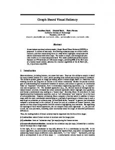
Image Compression based on Visual Saliency at Individual Scales Stella X. Yu1 and Dimitri A. Lisin2 1
Computer Science Department Boston College, Chestnut Hill, MA 02467, USA 2 VideoIQ, Inc. Bedford, MA 01730, USA
Abstract. The goal of lossy image compression ought to be reducing entropy while preserving the perceptual quality of the image. Using gazetracked change detection experiments, we discover that human vision attends to one scale at a time. This evidence suggests that saliency should be treated on a per-scale basis, rather than aggregated into a single 2D map over all the scales. We develop a compression algorithm which adaptively reduces the entropy of the image according to its saliency map within each scale, using the Laplacian pyramid as both the multiscale decomposition and the saliency measure of the image. We finally return to psychophysics to evaluate our results. Surprisingly, images compressed using our method are sometimes judged to be better than the originals.
1
Introduction
Typical lossy compression methods treat an image as a 2D signal, and attempt to approximate it minimizing the difference (e.g. L2 norm) from the original. By linearly transforming an image using an orthogonal basis (e.g. Haar wavelets), solutions of minimal difference can be computed by zero-ing out small coefficients [1, 2]. As there are many different zero-ing schemes corresponding to the same total difference, various thresholding techniques (e.g. wavelet shrinkage) that aim to reduce visual artifacts have been developed [3–6]. However, an image is not just any 2D signal. It is viewed by human observers. Lossy image compression should reduce entropy while preserving the perceptual quality of the image. Signal-based methods fall short of both requirements: zeroing out small coefficients aims at reducing pure signal differences instead of entropy, and reducing signal difference does not guarantee visual quality. Our work concerns the use of visual saliency to guide compression. This topic has been explored on multiple fronts, such as modifying the JPEG format [7], compressing salient and non-salient regions with separate algorithms [8], and applying saliency-based non-uniform compression to video [9]. Most saliency models yield a location map based on low-level cues [10], or scene context and visual task [11], treating scale like any other primary feature such as orientation, color, and motion. Computer vision algorithms often concatenate measurements at multiple scales into one feature vector without questioning its validity.
2
Stella X. Yu1 and Dimitri A. Lisin2
We first conduct an eye tracking experiment, and discover that human vision often attends to one scale at a time, while neglecting others (Sec. 2). We then develop a saliency-based compression scheme in which the entropy is reduced at each scale separately, using that scale’s saliency map (Sec. 3). We finally validate our approach in another psychophysical experiment where human subjects render their judgement of visual quality between pairs of briefly presented images (Sec. 4). Our compression results not only look better than the signal-based results, but, surprisingly, in some cases even better than the originals! One explanation is that our saliency measure captures features most noticeable in a single glance, while our entropy reduction aggressively suppresses the often distracting background, enhancing the subjective experience of important visual details.
2
Scale and Human Visual Attention
Our inspiration comes from studying change blindness [12]: When two images are presented with an interruption of a blank, the blank wipes out the retinal stimulation usually available during natural viewing, making the originally trivial change detection extremely difficult, even with repeated presentations. Using an eye tracker, we discover 3 scenarios between looking and seeing (Fig. 1): 1) Most detections are made after the gaze has scrutinized the change area. 2) If the gaze has never landed upon the area, seeing is unlikely. 3) Sometimes the gaze repeatedly visits the change area, however, the subject still does not see the change. Our gaze data reveals two further scenarios for the last case of no seeing with active looking. 1) For 80% of visits to the area of change, the gaze did not stay long enough to witness the full change cycle. As the retina is not receiving sufficient information regarding the change, blindness naturally results. 2) For the rest 20% of visits which involve 9 of 12 stimuli and 10 out of 11 subjects, the gaze stayed in the area more than a full cycle, yet the change still escaped detection. Those are true instances of looking without seeing [13].
1. looking and seeing
2. no looking, no seeing
3. active looking, no seeing
Fig. 1. Relationship between looking and seeing. A four-image sequence, I, B, J, B, is repeatedly presented for 250ms each. I and J denote images a major difference (the presence of a person in the white circle in this case), and B a blank. Shown here are 3 subjects’ gaze density plots as they search for the difference. Red hotspots indicate the locations that are most looked at. Only Subject 1 detected the change.
Lecture Notes in Computer Science
3
Fig. 2. The scale difference between fixations is more than 1.5 folds (solid lines) in 88% cases. The horizontal axis is for the size of change. The vertical axis is the size of the area examined in the fixation before entering (�) or after exiting (×) the change area. While the size here is determined based on manually outlined focal regions, similar results are obtained with synthetic stimuli varying only in the size dimension.
We examine the retinal inputs fixation-by-fixation. In most true instances of looking without seeing, the areas visited by the eye right before or after the change area tend to have features of a different scale from the change (Fig. 2). If at time t − 1 the subject is looking at a coarse-scale structure, he is likely to be oblivious to the change in a fine-scale structure at time t, and he tends to continue looking at a coarse-scale structure at time t + 1. In other words, when the visual system attends to one scale, other scales seem to be neglected.
3
Saliency and Compression
Our experiment suggests that human vision attends to one scale at a time, rather than processing all scales at once. This implies that saliency should be defined on a per-scale basis, rather than aggregated over all scales into a single 2D saliency map, as it is typically done [10]. We use the Laplacian pyramid [1] to define a multi-scale saliency map, and we use range filters [14] to reduce the entropy of each scale, applying more range compression to less salient features (Fig. 3). We adopt the Laplacian pyramid as both the multiscale signal decomposition and the saliency measure of the image, since the Laplacian image is the difference of images at adjacent scales and corresponds to center-surround filtering responses which indicate low-level feature saliency [10]. Step 1: Given image I and number of scales n, build Gaussian pyramid G and Laplacian pyramid L, where ↓ = downsampling, ↑ = upsampling Gs+1 =↓ (Gs ∗ Gaussian),
G1 = I,
s=1→n
(1)
Ls = Gs − ↑ Ls+1 ,
Ln+1 = Gn+1 ,
s=n→1
(2)
Stella X. Yu1 and Dimitri A. Lisin2
G′
L
L′
R
S
Decomposition
G
Normalization Saliency Fig. 3. Our image compression uses the Laplacian pyramid as both a signal representation and a saliency measure at multiple scales.
To turn the Laplacian responses into meaningful saliency measures for compression, we first normalize it (L → R) and then rectify it (R → S) using sigmoid transform with soft threshold m and scale factor α (Fig. 4). α controls saliency sharpness and is user-specified. We then use binary search to find the optimal m that satisfies the total saliency percentile p: If S = 1, p = 1, every pixel has to be maximally salient, whereas if p = 0.25, about 25% of the pixels are salient. Step 2: Given percentile p and scaling factor α, compute saliency S from L using a sigmoid with threshold m: �−1 � Rs −ms ,s=1:n (3) Ss = 1 + e− α ( ) X X |Ls | ms = arg (4) Ss (i; ms ) = p · 1 , Rs = max(|L s |) i i We modify Laplacian L by range filtering with saliency S. Range compression replaces pixel i’s value with the weighted average of neighbours j’s, larger weights for pixels of similar values [14]. Formulating the weights W as a Gaussian of value differences, we factor saliency S into covariance Θ: High saliency leads to low Θ, hence high sensitivity to value differences, and value distinction better preserved. The maximal amount of compression is controlled by the range of Laplacian values at that particular scale (Eqn. 7).
Range Compression Construction
4
Lecture Notes in Computer Science
5
Saliency S give α and m
1 α=0.01 m=0.40
α=0.05 m=0.50
0.8
α=0.10 m=0.60
0.6 0.4 0.2 0 0
0.2 0.4 0.6 0.8 Normalized Laplacian Response R
1
Fig. 4. Sigmoid function rectifies the Laplacian to become a saliency measure. m is a soft threshold where saliency becomes 0.5. α controls the range of intermediate saliency values. Low α forces a binary (0 or 1) saliency map.
1 Relative Maximal Bin Size
Normalized Bin Size
1 α=0.01 m=0.40
0.8 0.6
α=0.05 m=0.50 0.4
α=0.10 m=0.60
0.2 0
image Lena 0.8 0.6 0.4 0.2 0
0
0.2 0.4 0.6 0.8 Normalized Laplacian Response R
1
1
2
3 Scale
4
5
scale-adaptive binning
value-adaptive binning 0.2
L
2
image Lena
L’
Normalized Histograms
2
L
3
L’
3
0.1
0 −50
0
50
Fig. 5. The Laplacian is range compressed as a signal subject to itself as saliency measure. The reduction in entropy is achieved by implicit adaptive binning in the histograms. We can have some idea of the bin size by examining the standard deviation √ √ 1 of W : Θ 2 = 1 − S · (max(L) − min(L))/β. The first factor 1 − S makes the bin dependent on the value, whereas the second (max(L) − min(L))/β makes it dependent on the scale, for the range of L naturally decreases over scale.
6
Stella X. Yu1 and Dimitri A. Lisin2
Step 3: Given S, neighbourhood radius r and range sensitivity factor β, generate a new Laplacian pyramid L′ by spatially-variant range filtering of L: P j∈N (i,r) Ls (j) · Ws (i, j) ′ P , L′n+1 = Ln+1 , s = 1 : n (5) Ls (i) = W (i, j) s j∈N (i,r) Ws (i, j) = e−
(Ls (i)−Ls (j))2 2Θs (i)
Θs (i) = (1 − Ss (i)) ·
�
(6)
,
max(Ls ) − min(Ls ) β
�2
(7)
The nonlinear filtering coerces the Laplacian values towards fewer centers (Fig. 5). It can be understood as scale- and value-adaptive binning: As the scale goes up, the bin gets smaller; as the value increases, the saliency increases, and the bin also gets smaller. As the value distribution becomes peakier, the entropy is reduced and compression results. The common practice of zero-ing out small values in Laplacians or wavelets only expands the bin at 0 while preserving signal fidelity, whereas our saliency regulated local range compression adaptively expands the bin throughout the levels while preserving perceptual fidelity. Finally, we synthesize a new image by collapsing the compressed Laplacian pyramid (Fig. 3 G′ , L′ ). Note that L and L′ look indistinguishable, whereas nonsalient details in G are suppressed in G′ . Step 4: Construct the compressed image J by collapsing the new Laplacian L′ : G′s = L′s + ↑ G′s+1 , G′n+1 = L′n+1 , s = n → 1; J = G′1
4
(8)
Evaluation
Lossy image compression sacrifices quality for saving bits. Given infinite time to scrutinize, one is bound to perceive the loss of details in a compressed image. However, in natural viewing, instead of scanning the entire image evenly, we only dash our eyes to a few salient regions. Having developed an image compression method based on human vision, we now return to it to evaluate our results. We carry out two-way forced choice visual quality comparison experiments using 12 standard test images (Fig. 8). Using our method, we generate 16 results per image with α ∈ {0.01, 0.1}, p ∈ {0.25, 0.5}, r ∈ {3, 6} β ∈ {5, 10}. For each image, we choose 3 compression levels that correspond to minimal, mean and maximal JPEG file sizes. For each level, we find a signal-compressed version of the same JPEG file size but reconstructed from zero-ing out sub-threshold values in the Laplacian pyramid. The threshold is found by binary search. We first compare our results with signal-based results (Fig. 6). Each comparison trial starts with the subject fixating the center of a blank screen. Image
Lecture Notes in Computer Science
7
signal-based compression:
our perception-based compression:
Quality Rating w.r.t. Signal Compression
visual quality comparison:
1
0.5
0 0
0.2 0.4 0.6 0.8 Compression Percentage
1
Fig. 6. Comparison of signal-based compression (row 1) and our perception-based compression (row 2). Row 3 shows a plot of quality ratings of our results for different compression ratios. The quality rating is the fraction of subjects who judged our results to be better than those produced by the signal-based algorithm. Each dot in the plot represents a quality rating of the perception-based compression of a particular image resulting in the compression ratio given by the horizontal axis. Our results are better in general, especially with more compression.
8
Stella X. Yu1 and Dimitri A. Lisin2 wavelet compression:
our compression:
Fig. 7. Our results (row 2) are better than compression by Daubechies 9-tap/7-tap wavelet with level-dependent thresholding (row 1) for the same JPEG file size.
1 is presented for 1.2s, followed by a gray random texture for 0.5s, image 2 for 1.2s, and random texture again till a keypress indicating which one looks better. The occurrence order within each pair is randomized and balanced over 15 naive subjects, resulting in 30 trials per pair of images. Our quality rating is determined by the percentage of favorable votes for our method: 0.5 indicates that the images from two methods have the same visual quality statistically, whereas a value greater(less) than 0.5 means our results are better(worse). The visual quality of our results is better overall, especially with heavier compression. We have also computed wavelet compression results with various settings: Haar vs Daubechies 9-tap / 7-tap wavelet, global- vs. level-dependent thresholding via Birge-Massart strategy. They have their own characteristic patterns in quality loss over heavy compression. Our compressed images degrade more gracefully than those as well (Fig. 7). Finally, we compare our results at the best quality level to the original images (Fig. 8). 1) At a short exposure, our results are entirely indistinguishable from the original; 2) At a medium exposure, ours are better than the original! The enhancement is particularly strong for face images. 3) At a long exposure, our results become slightly worse. Such exposure-dependence in fact supports the validity of our saliency model: Our method captures visual features of the firstorder significance at the cost of losing details of the second-order significance. At low levels of compression, our method produces an air-brush effect which emphasizes strong straight edges and evens out weak and curly edges, lending
Lecture Notes in Computer Science
Quality Rating w.r.t. Original
1
9
0.4 sec: mean = 0.50 = 0.5, p = 1.00 0.8 sec: mean = 0.52 > 0.5, p = 0.78 1.2 sec: mean = 0.48 < 0.5, p = 0.90
0.5
0 1
1
2
3
4
I: original image
2
3
5
4
5
6
6 7 Image
8
7
J: our compression
9
10 11 12
8
9
10
11
12
I − J: difference
Fig. 8. Comparison between the originals and our compressed results (row 1) on 12 test images (row 2) at the exposure times of 0.4, 0.8, and 1.2 seconds, with p-values from two-, right-, and left-tailed one-sample t-tests between the means and the equal quality level 0.5. Our results are equally good at the short exposure (too short for anyone to notice any differences), better at the medium exposure, and worse at the long exposure (long enough to notice the distinction in richness). The enhancement at the medium exposure is most positive in image 2 (row 3), and most negative in image 10 (row 4), where the air-brush effect makes the facial characteristics clearer and the pepper textures disturbingly fake.
10
Stella X. Yu1 and Dimitri A. Lisin2
more clarity to a face image while destroying the natural texture in a pepper image (Fig. 8 bottom). At higher levels of compression (Fig. 7), our method creates the soft focus style used by photographer David Hamilton, which blurs the image while retaining sharp edges. Summary. Our human vision study suggests that a saliency model must treat each scale separately, and compression must preserve salient features within each scale. We use the Laplacian pyramid as both signal representation and saliency measures at individual scales. Range compression modulated by saliency not only results in entropy reduction, but also preserves perceptual fidelity. This can be viewed as value- and scale-adaptive binning of the distributions, an elegant alternative to various thresholding strategies used in wavelet compression. Our validation with human viewers indicates that our algorithm not only preserves visual quality better than standard methods, but can even enhance it. Acknowlegements. This research is funded by NSF CAREER IIS-0644204 and a Clare Boothe Luce Professorship to Stella X. Yu.
References 1. Burt, P., Adelson, E.H.: The Laplacian pyramid as a compact image code. IEEE Trans. Communication 31 (1983) 2. Mallat, S.: A theory for multiresolution signal decomposition: The wavelet representation. PAMI (1989) 3. Simoncelli, E., Adelson, E.: Noise removal via Bayesian wavelet coring. In: IEEE International Conference on Image Processing. Volume 1. (1996) 4. Donoho, D.L.: De-noising by soft-thresholding. IEEE Trans. Information Theory 4 (1995) 613–27 5. Chambolle, A., DeVore, R.A., Lee, N., Lucier, B.J.: Nonlinear wavelet image processing: variational problems, compression, and noise removal through wavelet shrinkage. IEEE Trans. Image Processing 7 (1998) 319–35 6. DeVore, R., Jawerth, B., Lucier, B.: Image compression through wavelet transform coding. IEEE Transactions on Information Theory 32 (1992) 7. Golner, M.A., Mikhael, W.B., Krishnang, V.: Modified jpeg image compression with region-dependent quantization. Circuits, Systems, and Signal Processing 21 (2002) 163–180 8. Lee, S.H., Shin, J.K., Lee, M.: Non-uniform image compression using biologically motivated saliency map model. In: Intelligent Sensors, Sensor Networks and Information Processing Conference. (2004) 9. Itti, L.: Automatic foveation for video compression using a neurobiological model of visual attention. IEEE Trans. Image Processing 13 (2003) 669–673 10. Itti, L., Koch, C.: Computational modelling of visual attention. Nature Neuroscience (2001) 194–203 11. Torralba, A.: Contextual influences on saliency. In Itti, L., Rees, G., Tsotsos, J., eds.: Neurobiology of Attention. Academic Press (2004) 586–93 12. Rensink, R.A.: Change detection. Annual Review of Psychology 53 (2002) 4245–77 13. O’Regan, J.K., Deubel, H., Clark, J.J., Rensink, R.A.: Picture changes during blinks: looking without seeing and seeing without looking. Visual Cognition 7 (2000) 191–211 14. Tomasi, C., Manduchi, R.: Bilateral filtering for gray and color images. In: International Conference on Computer Vision. (1998)