image compression versus matching accuracy

Michael Kiefner

IMAGE COMPRESSION VERSUS MATCHING ACCURACY Michael Kiefner*, Michael Hahn** * Z/I Imaging, Germany [email protected] ** University of Applied Sciences, Stuttgart, Germany Faculty of Surveying and Geoinformatics [email protected] Working Group I/2

KEY WORDS: JPEG, Wavelet and Fractal Compression, Matching Accuracy, Compression Ratio, PSNR

ABSTRACT The improvements of aerial image scanners regarding the scan resolution and in particular the development of new digital cameras (e.g. the DMC of Z/I Imaging) comes along with the production of Gigabytes of image data. To handle these big data sets image compression algorithms are applied. The number of developed image compression procedures is growing and investigations of the consequences for photogrammetric image processing are becoming very important for users of compressed image data. This paper investigates theoretically and experimentally the impact of different compression algorithms on image matching quality. The focus is laid on automated point transfer using the area based least squares matching principle. Other automated processes like aerial triangulation, DTM acquisition and relative orientation often directly rely on the results of the employed point transfer process thus consequences on these processes are inferable. In the experimental investigations simulated stereo imagery and real stereo image pairs are taken into account. Representative algorithms of three different compression methods, the JPEG, Wavelet and Fractal compression, are used to verify and quantify the theoretically found relation between matching accuracy and compression ratio. Regarding the peak-signal-to-noise-ratio (PSNR) of the images induced by compression, Wavelet compression proves to be superior to JPEG and Fractal compression. With respect to the success rate and matching accuracy of point transfer a continuous decrease is to be expected with increasing compression rate. But unlike the PSNR results a changed ranking of the compression methods has to be observed. The highest matching success quotas combined with the most precise point transfer were achieved with the JPEG algorithm. Wavelet compression followed quite closely but Fractal compression dropped down significantly, therefore is not recommended for photogrammetric applications. For high precision point transfer, which is required in most photogrammetric applications, the investigations show that compression ratios not lower than 1:5 can be tolerated. Using images with lower compression ratios will produce point transfer errors above 0.1 to 0.2 pixels.

1 INTRODUCTION To deal with the enormous disk space requirements of photogrammetric image data sets various compression algorithms are in use. Up to now algorithms based on JPEG compression are the most commonly used compression software but Wavelet based algorithms are not far behind any more. A third group of compression procedures are based on Fractal compression techniques. Often high compression rates are anticipated from developments in this area. In the following we do not want to review the compression techniques. Instead we refer to Pennebaker and Mitchel, 1993, Barnsley and Hurd, 1993, Louis et al., 1994 and Saupe et al., 1997. An overview can be found in Hahn and Kiefner (1998) in which we started reporting about this research. Empirical studies on the dependency of photogrammetric accuracy and image compression started some years ago. Most investigators used JPEG compression and proposed, for example, compression ratios of 1:10 (Jaakola and Orava, 1994) or 1:12,5 (Novak and Shahin, 1995). Others investigated the accuracy of DTMs made with compressed images and related the loss of DTM accuracy to JPEG quality factors (Reeves et al., 1997, Robinson et al., 1995). The aim of this research is to extend those studies by taking the other mentioned compression techniques into account. Because compression rates of 10 or more can not be achieved by lossless compression, at least not with photogrammetric images, our investigations deal only with lossy compression techniques.

316

International Archives of Photogrammetry and Remote Sensing. Vol. XXXIII, Part B2. Amsterdam 2000.

Michael Kiefner

In a broad variety of applications of general image processing often JPEG compression ratios in the order of 1:10 are recommended. Even though JPEG compression ratios of 1:40 or even smaller can be achieved, subjective differences are readily discernible at compression rates in the order of 15. However careful scrutiny will reveal differences in the compressed images at much lower compression rates. Wavelet compression generally produces less visible image distortions than JPEG compression thus a higher compression rate may be used without producing a significant derogation of the visual impression of the compressed image. Furthermore, the achievable Wavelet compression rates are a multiple of that of JPEG compression as outlined in Thierschmann et al.(1997). The fact that compression induced distortions might not be visible should not be misinterpreted by assuming that therefore the consequences for photogrammetric applications are negligible. First results using all three compression techniques indicated errors of transferred point locations of 0.5 pixels at compression ratios of 1:10 (Hahn and Kiefner, 1998). Before developing a model for relating compression and accuracy in Section 3, we will examine the impact of compression on the gray value image and show that the effect of JPEG, Wavelet and Fractal compression can be properly approximated by a Gaussian distribution. Section 4 reports about aspects of image quality under the influence of compression. The images and point transfer methods used in the experimental investigation are presented in Section 5. The results of a series of experiments using scanned aerial images, images taken by the digital airborne camera system DPA and images recorded with the spaceborne MOMS system are reported in Section 6. We conclude with a summary of our findings, including recommendations for the use of compression algorithms in digital photogrammetry.

2 DISTRIBUTION OF COMPRESSION NOISE

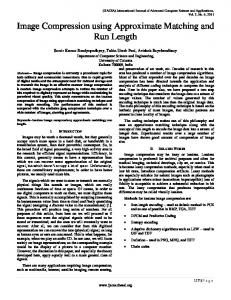
Figure 1 shows the impact of the compression algorithms at full quality. Most compression algorithms use a quality parameter to specify the impact of compression and with that indirectly the compression ratio. Full quality means that ideally no information should be lost and the gray values of an image compressed at full quality should not differ significantly from the original image. The results obtained for the MOMS image are shown in Figure 1. The chart reveals two important issues. Firstly, compression at full quality which may result in compression ratios in the order of 1:1.3 to 1:2 or 1:3 produces a very small percentage of gray value differences of 1 or 2 gray levels for Wavelet and JPEG compression which fits to the expectation. The value 128 on the horizontal axis of the chart represents a gray value difference of 0. More surprising is the result of the Fractal compression algorithm. Obviously the differences are much bigger than for the other two methods and the compression algorithms produces a systematic gray value shift of nearly 2 gray levels. Because the matching procedure (Section 5) is

500000

0 122

124

126

128

130

132

134

gray values

Figure 1: Histogram of the gray value differences between the original and the compressed MOMS image using full quality

Histogram of the differences (MOMS, JPEG)

frequency of occurance

Three image data sets are used in the experiments. The first is a spaceborne MOMS image with a ground pixel size of 17 m. The second image is recorded by the DPA camera which is an airborne line imaging scanner. The third image is a digitized photographic aerial image. The latter both have a ground pixel size of 80 cm.

frequency of occurrence

The theoretical framework used in this paper is related to least squares point transfer with two shift parameters: the parallaxes in x and y direction of the image coordinate system. This framework requires that image noise can be modeled as Gaussian noise. Transferring the Gaussian noise assumption to compressed images requires that JPEG, Histogram of Differences Wavelet and Fractal compression can be modeled as (MOMS, full quality) degrading the image by the addition of Gaussian noise. This 2500000 has to be true for all three compression techniques over a large region of different compression ratios. To prove this 2000000 JPEG assumption the gray level differences between the original 1500000 Wavelet image and the compressed images are calculated which 1000000 Fraktal represent compression noise.

2000000 1:78,56 1500000

1:39,03 1:33,31

1000000

1:22,81 1:13,11

500000

1:9,36 0 122

1:3,63 124

126

128

130

132

134

1:2,05

gray values

Figure 2: Differences between original and compressed images for a series of different compression ratios using the JPEG algorithm


317

Michael Kiefner

invariant to a gray scale shift this systematic error caused by the Fractal compression algorithm is without significance for this investigation. A histogram of the differences between original and JPEG compressed images generated for various compression ratios shows Gaussian curves of different width (Figure 2). The series of compression ratios ranges from 1:2 to 1:78 whereby the achieved rate of nearly 80 is a remarkably high JPEG rate. The figure indicates that the distribution with the differences is close to the Gaussian distribution. The corresponding histograms for the other two compression methods are very similar to those plotted on Figure 2 with the peculiarity that the Fractal results show up with an additional offset. It should be noted that the used images have to be big enough (1000 by 1000 pixels or more) to have a large statistical sample. Histograms of differences determined from smaller fragments of images (e.g. 200 by 200) often are show up with a distribution which is more peaked than the Gaussian distribution. For JPEG compression this effect is caused by a loss of high frequencies and the appearance of artifacts such as block boundaries (Reeves and Hahn, 1997).

3 A MODEL FOR RELATING COMPRESSION AND ACCURACY The theoretical framework used in this paper to relate compression and accuracy is based on the least squares approach of area based image matching. The idea is to formulate a model which allows to predict the accuracy of point transfer to a given measure for image compression. A proper measure for image compression is compression noise. As outlined in the previous section compression noise can be approximated by additive Gaussian noise. The theoretical accuracy of point transfer using least squares matching with two parallax unknowns px and py is given by the well-known formula 2  px  σˆ 2  σ D  = n  f X   py  m  σ f X fY

with

m σˆ n2

X Y

Y

   

−1

(3.1)

= number of pixels in the matching window = variance of image noise

σ ,σ D(.) 2 fX

σf f σ 2f

2 fY

= mean sum of squared gradients of the image = covariance matrix of the parallaxes

Assuming that image noise is substituted by the superimposition of compression noise and image noise or just by dominating compression noise, equation (3.1) can be interpreted in the light of image compression. If the mean sum of squared gradients are determined from the uncompressed image there is no impact of compression on equation (3.1) other than compression noise. Assuming further that the off-diagonal elements of the 2 x 2 matrix in (3.1) are small compared to the mean sum of the squared gradients the following formula is obtained

σˆ pxy =

Compression noise

σˆ cn

(σˆ

2 px

+ σˆ 2py 2

)=

σˆ cn 2m

 1 1  + 2  σ 2f  X σ fY

   

(3.2)

and the remaining expression in (3.2) which relates to the mean sum of squared gradients and

the window size are the two parameters which influence the estimate of the achievable accuracy of point transfer using compressed images. To verify this model rms errors can be computed by matching a simulated stereo image pair for which the true parallaxes are known. In a second step the investigations then will be extended to real image pairs of the above mentioned image data sets. But before we continue in this direction we will have a closer look at the quality of compressed images, in particular, to the entropy and the PSNR.

4 QUALITY OF COMPRESSED IMAGES A frequently used measure for the quality of images is the entropy. It is defined by the following formula: 255

H = − ∑ p(g) log 2 (p(g)) g =0

318


(4.1)

Michael Kiefner

For computing the entropy H the probabilities or relative frequencies of the different grey values have to be determined first to be entered into to equation (4.1). The entropy calculated for the three image data sets and for all three compression methods is given in Table 1. The column entitled ‘Min’ lists the minimum entropy obtained with the highest compression rate achieved by the three compression schemes. For images with 8 bit information and the entropy should be close to 8. From Table 1 can be seen that the aerial images (RMK Top camera) possess the highest entropy H(RMK) = 7.7 followed by significantly lower entropy values of H(DPA) = 6.2 and H(MOMS) = 5.8. This means the image data which enter into the point transfer investigations differ considerably regarding the information content measured by the entropy. Remarkable is that there is a minor loss of entropy between the original images and the highly compressed images. Significant differences between the three compression methods can not be observed in the entropy values obtained for the compressed images.

Camera

Method JPEG Fraktal Wavelet JPEG Fraktal Wavelet JPEG Fraktal Wavelet

RMKTOP

DPA

MOMS

Original Image

Min 7,62 7,58 7,68 5,70 6,19 6,20 5,43 5,70 5,73

7,70

6,21

5,78

Table 1: Entropy for the different images and the three compression methods. For comparison the entropy for the original images is listed also.

A second measure for image quality is the peak-signal-to-noise-ratio. In Netravali and Haskell (1994] the PSNR is defined as follows:

 2552   PSNR = 10 * log10   MSE 

(4.2)

with

MSE =

N M 1 *∑∑ (g ijo − gijc )2 N*M i =1 j =1

(4.3)

g ijo are the gray values of the original and g ijc the gray values of compressed images. A dependency of the PSNR on the

1. 2. 3.

Wavelet JPEG Fractal

PSNR of all compression methods and image types

70 60 PSNR [dB]

compression method and compression ratio is to be expected. The PSNR values obtained for all three compression algorithms over a multitude of compression ratios are plotted in Figure 3. The PSNR decreases largely for compression rates up to 5. For higher rates the curves are rather flat. Looking at each specific image type individually shows the following ranking between the algorithms:

50

JPEG MOMS

40

Wavelet Fractal

DPA

30 RMKTOP

20 0

5

10

15

20

25

Compression Ratio [1:X] The PSNR curves of Wavelet compression are always a little bit above those of JPEG. The lowest curves are those Figure 3: PSNR values for JPEG, Wavelet and Fractal obtained by Fractal compression. A closer look at the results compression shows that the differences between JPEG and Wavelet are quite small and only Fractal compression results are significantly behind. This coincides with our observations about the compression noise distribution (cf. Section 2). Another finding of Figure 3 is that the PSNR depends stronger on the image signal than on the used compression algorithm. While the PSNR curves follow nearly the same trend for each compression method the curves are highest for the low entropy MOMS images and lowest for the high entropy RMK images.

5 STRATEGIC ASPECTS OF POINT TRANSFER The computation of entropy and PSNR has given an impression of the impact of the different compression methods on the image quality. With the model proposed in Section 3 the loss of image quality can be related to geometric accuracy of point transfer. Point transfer procedures employ a certain matching routine and moreover may include control strategies which are used to eliminate matches which do not fit to the expectation. Before we discuss the experiments on


319

Michael Kiefner

matching accuracy under compression we first outline the transfer methods and give some more details about the used images. 5.1 Point Transfer Basis of the point transfer procedure is area based least squares matching with the standard six geometric parameters of an affine transformation. For point transfer a point in the matching window is selected and transferred to the other image. For convenience mostly the center point in the matching window is used as reference or transfer point. Two strategic options are implemented in the transfer process. The first option called “Standard LSM” transfers the reference point from the master image to the slave image. If matching converges as expected and the plausibility check by cross correlation indicates a successful match then the point is transferred. The second option is “LSM with self control” which takes an additional check into account. A point transferred by Standard LSM is transferred back to the master image in a second match with an exchanged role of master and slave image. If the second match is successful too and the back transferred point location does not differ significantly (commonly 0.1 pixels deviation is tolerated) from the reference location of the point in the master image then this check is passed and the point is considered to be successfully transferred. From experience we know that points transferred with the self control mechanism are more reliable, i.e. matching errors appear not as often as in results obtained by Standard LSM. For investigating the influence of the compression algorithms a sufficiently large sample size of points is used. Reference points for point transfer are simply defined by a regular grid. Precisely a sample of 3481 points is used in each series of the experiments. 5.2 More Details about the Used Image Data With a real stereo image pair it is difficult to separate the influence of image compression on matching accuracy from the effects induced by a imperfect approximation of the geometric relation between the two images. Therefore we carry out the investigations with simulated stereo pairs and with real stereo image pairs. The simulated stereo pair is created from one real image. A 1500 by 1500 pixel image is extracted from the original image. By cutting out a second image with an offset of one pixel in x- and y-direction a simulated stereo partner of the same size is obtained. Afterwards both images were put through the compression algorithms. For each of the three compression methods a series of compressed images with different compression ratios are generated. For point transfer the compressed images are decompressed to be available as a standard image matrix. For the investigations with real stereo images, pairs of images of the already mentioned MOMS, DPA and RMK cameras are used (cf. Section 2). To have a reference for point transfer with compressed images the points transferred in the uncompressed image pairs are computed. The differences between point transfer in compressed and uncompressed images show the influence of the compression algorithms.

6 MATCHING ACCURACY IN COMPRESSED IMAGES The results using simulated stereo images are discussed briefly in this section since that part of the investigation has already been presented in a previous paper (Hahn and Kiefner, 1998). The emphasis will be laid on investigations with real image pairs. 6.1 Investigations with Simulated Stereo Images

320

0,5 Deviation [pixel]

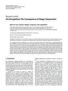
Point transfer in compressed images has been carried out for a series of compression ratios and all three image data sets. Figure 4 shows the results for the RMK Top image. The deviations between the match results and the known true parallaxes (rms values) are plotted with respect to its corresponding compression ratios. What may be noticed first by looking at the chart is that JPEG compression delivered more accurate results than Wavelet and Fractal compression. The JPEG curve is below the other both for almost the full range of compression ratios. An error level of 1/10 of a pixel is passed with JPEG images at a ratio of 1:7 whereas the same error is already obtained with Wavelet compression at a ratio of 1:4. For Fractal compression this mark

Standard Deviation σ xy (RMK, Standard LSM) 0,6

0,4 JPEG Wavelet

0,3

Fractal 0,2 0,1 0 0

2

4

6

8

10

12

14

16

Ratio [1:X]

Figure 4: Point transfer errors for different compression ratios (RMK Top, Standard LSM))


Michael Kiefner

is passed somewhere between the rations 1:3 and 1:4. The exact compression rates for the 1/10 of a pixel point transfer error level are listed in Table 2 for all three image types and for both point transfer strategies. Figure 4 shows the typical behavior of the error curves for accuracy for all three image data sets. In all images and for both point transfer strategies the ranking of the compression algorithms is observed: Compression Camera

1. 2. 3.

JPEG Wavelet Fractal

The higher compression rates for point transfer mode LSM with self control satisfies the expectation. The reason is the elimination of a certain percentage of points transferred by Standard LSM which do not satisfy the requirements of self control. For compression ratio of 1:5 the loss of transferred points is between 5% and 10% for all three image types. The higher the compression rates the bigger is the difference between the two transfer methods.

Ratio 1:X Standard LSM With Self Control JPEG 5,6 6,7 RMK Top Wavelet 3,9 5 3 4,2 Fractal JPEG 3,8 4,5 DPA Wavelet 2 2,9