Image Database Retrieval Utilizing Affinity Relationships Mei-Ling Shyu
Shu-Ching Chen, Min Chen, Chengcui Zhang Kanoksri Sarinnapakorn
Department of Electrical and Distributed Multimedia Information System Laboratory Department of Electrical and Computer Engineering School of Computer Science Computer Engineering University of Miami Florida International University University of Miami Coral Gables, FL 33124, USA Miami, FL 33199, USA Coral Gables, FL 33124, USA 1-305-284-5566
1-305-348-3480
1-305-284-5566
[email protected]
{chens, mchen005, czhang02}@cs.fiu.edu
[email protected]
ABSTRACT Recent research effort in Content-Based Image Retrieval (CBIR) focuses on bridging the gap between low-level features and highlevel semantic contents of images as this gap has become the bottleneck of CBIR. In this paper, an effective image database retrieval framework using a new mechanism called the Markov Model Mediator (MMM) is presented to meet this demand by taking into consideration not only the low-level image features, but also the high-level concepts learned from the history of user’s access pattern and access frequencies on the images in the database. Also, the proposed framework is efficient in two aspects: 1) Overhead for real-time training is avoided in the image retrieval process because the high-level concepts of images are captured in the off-line training process. 2) Before the exact similarity matching process, Principal Component Analysis (PCA) is applied to reduce the image search space. A training subsystem for this framework is implemented and integrated into our system. The experimental results demonstrate that the MMM mechanism can effectively assist in retrieving more accurate results from image databases.
Categories and Subject Descriptors H.3.3 [Information Storage and Retrieval]: Information Search and Retrieval – Retrieval Models.
General Terms Algorithms, Experimentation.
Keywords Content-based Image Retrieval, Markov (MMM), and Principal Component Analysis.
Model
Mediator
Permission to make digital or hard copies of all or part of this work for personal or classroom use is granted without fee provided that copies are not made or distributed for profit or commercial advantage and that copies bear this notice and the full citation on the first page. To copy otherwise, or republish, to post on servers or to redistribute to lists, requires prior specific permission and/or a fee. MMDB’03, November 7, 2003, New Orleans, Louisiana, USA. Copyright 2003 ACM 1-58113-726-5/03/0011…$5.00.
1. INTRODUCTION The explosion of image databases and the inefficiency of textbased image retrieval have created an urgent need for effective approaches in image database retrieval. Content-Based Image Retrieval (CBIR) approaches have been actively researched to address this need. These approaches utilize the features that are inherent in the images, such as color [1], shape [2] and texture [3], for retrieval purposes. However, an impediment to research on CBIR is the lack of mapping between the high-level concepts and the low-level features. Currently, research efforts to address this issue fall into two major categories: region-based image retrieval and relevance feedback (RF). Region-based retrieval attempts to overcome the deficiencies of global feature matching processes by representing images at the object level, which is achieved by segmenting an image into a number of regions (i.e., a group of connected pixels which share common properties) and then the features of each region can be extracted and compared [4]. The object-level representation is considered a more natural way to capture human’s perception. However, currently, there is hardly any unsupervised segmentation algorithm that can partition an image into regions/objects perfectly, especially when the image database contains a large collection of heterogeneous images. Therefore, the inaccurate object-level representation may result in poor retrieval performance. Another major approach to capture the semantic contents of images is relevance feedback (RF) [5]. Relevance feedback is an interactive process used in image retrieval systems, which refines the query performance based on the user’s feedback on the quality of the previous query results performed by the system. Most of the relevance feedback research work has been carried out in two approaches: query point movement and re-weighting [6]. However, due to the fact that the metric dynamically depends upon the user’s feedback and the context, how to provide real-time learning capability of the distance metric or feature space transformations based on the users’ interactions is crucial and remains an open issue. In this paper, a novel content-based image retrieval system that utilizes not only the low-level features of the images but also the high-level user concepts such as the affinity relationships among the images in the image retrieval process is proposed. The central core of the proposed CBIR system is the Markov Model Mediator (MMM) mechanism, which has been applied to multimedia database management [11] and document management on the
World Wide Web (WWW) [12]. The MMM mechanism adopts the mediator concept and the Markov model framework. A mediator is defined as a program that collects data from one or more sources, combines the data for processing, and yields the resulting information [7]. Markov model is a well-researched mathematical construct for analyzing complicated systems and has been used in lots of research work including Markov Random Field Models [8], and Hidden Markov Models (HMMs) [9]. Especially, HMMs have been integrated into multimedia domain [10]. In the proposed framework, the high-level user concepts are captured through the training process. Instead of learning and interpreting user’s preferences through on-line user feedback, the relative affinity relationships among images in the image database are calculated off-line via the user access patterns and access frequencies from the training data, which serves as an indication of users’ high-level concepts in our system. This approach provides the capability to reduce the gap between low-level features and high-level concepts without sacrificing the system’s efficiency. In addition, for the sake of retrieval efficiency, Principal Component Analysis (PCA) is integrated into our proposed framework as the pre-filtering phase. Different from the approach proposed in [18], we avoid the expensive distance computation by utilizing the principal component scores to identify the images in the desired candidate image pool, and the distance computation is required only for those images in the candidate image pool. In order to test the performance of the proposed framework, a training subsystem has been implemented to collect the user access patterns and access frequencies, which is integrated into our system [20]. The remainder of this paper is organized as follows. In Section 2, the architecture of the proposed framework is introduced, followed by the detailed discussions for each important component, such as feature extraction process, training process, and retrieval process as well. Section 3 presents the system implementation and our experimental results in applying the proposed framework to content-based image retrieval. The experimental results demonstrate that our framework can assist in retrieving more accurate results for user queries. A brief conclusion is given in Section 4.
2. ARCHITECTURE OF THE PROPOSED FRAMEWORK The architecture of the proposed framework is shown in Figure 1. As can be seen from this figure, our proposed framework is divided into three major components based on their functionalities, namely image feature extraction process, training process, and retrieval process. In our framework, not only the low-level features (e.g., color) and the mid-level features (e.g., object locations), but also the high-level concepts learned from the off-line training process are used in the image retrieval process. Moreover, instead of conducting the exact similarity matching process in the whole database scope, a pre-filtering process using PCA is applied to reduce the search space. Hence, the retrieval process consists of the pre-filtering process and similarity matching process. In the following three subsections, each component and the relationships among the components are presented in details.
Retrieval Process
Image Feature Extraction
Pre-filtering Process
Training Process
Similarity Matching Process
Figure 1: Architecture of the proposed framework
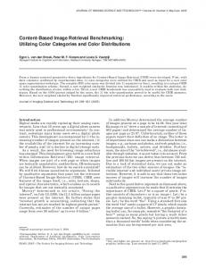
2.1 Image Feature Extraction Component The features of color information and object location information for the images in the image database are both considered in our proposed framework. The HSV color space is used to obtain the color feature for each image due to the following two reasons: (1) it is perceptual and a proven color space particularly amenable to color image analysis [19], and (2) it has shown in the benchmark results that the color histogram in the HSV color space has the best performance [13]. For object location information, the SPCPE algorithm proposed in [14] is used, where each object is covered by a rectangle since the minimal bounding rectangle (MBR) concept in R-tree [15] is adopted. In addition, the centroid point of each object is used for space reasoning so that each object is mapped to a point object. In this study, our main focus is not to explore the most appropriate features for image retrieval. Instead, we would like to evaluate the performance of the MMM mechanism and to reduce the feature space. Hence, each image has a feature vector of twenty-one elements, where twelve are for color descriptions and nine are for location descriptions. Based on the combinations of different ranges of the hue (H), saturation (S), and the intensity values (V), the color features ‘black’ (black), ‘white’ (w), ‘red’, ‘red-yellow’ (ry), ‘yellow’ (y), ‘yellow-green’ (yg), ‘green’ (g), ‘green-blue’ (gb), ‘blue’ (b), ‘blue-purple’ (bp), ‘purple’ (p) and ‘purple-red’ (pr) are considered. For any color whose number of pixels is less than 5% of the total number of pixels, its corresponding position in the feature vector has the value 0 since we treat it as non-important. Otherwise, the corresponding percentage of that color component is put in that position. For the location descriptions, each image is divided into 3×3 equal-sized reference regions that are ordered from left to right and top to bottom as L1, L2, L3, L4, L5, L6, L7, L8, and L9 (as shown in Figure 2). The value 1 is assigned to a region when there is an object in the image whose centroid falls into that reference region; and 0 otherwise. Moreover, an object will be ignored if its area is less than 2% of the total image area. When it is necessary, each image can be divided into a coarser or finer set of regions. 50
Centroid
100
150
200
250 50
100
150
200
250
300
350
Figure 2: Object locations and their corresponding regions In order to capture the appearance of a feature in an image, a feature matrix B is defined in the way that its rows are all the distinct images and columns are all the distinct features, where the
image is 1. It is worth mentioning that our framework is flexible in terms of the update on the feature matrix B. Any normalized vector-based image feature sets can be used to construct the B matrix. Table 1 illustrates the normalized feature vectors of the sample images in Figure 3.
value in the (p, q) entry is greater than zero if feature q appears in image p, and zero otherwise. We consider that the color and object location information are of equal importance. That is, the color features are normalized and their sum equals 0.5, and the location features are normalized and their sum is 0.5. Hence, each value indicates the probability of a feature observed from an image and the sum of the probabilities of all the features of the
Figure 3: Three sample images (Image 1 – Image 3) Table 1: B matrix - Normalized image feature vectors of the sample images black
w
Image 1 0.14 0.04 Image 2
0
0
Image 3 0.15 0.17
red
ry
y
yg
g
gb
b
bp
p
pr
L1 L2 L3 L4
L5
L6 L7
0
0
0
0
0
0.08
0
0.24
0
0
0 0.25 0
0
0
0
0 0.25 0
0.04
0
0 0.17 0.29
0
0
0
0
0
0 0.25 0
0
0.25
0
0
0
0
0.04 0 0.07 0.07
0
0
0
0
0
0
0
0.5
0
0
0
0
0
2.2 Training Process Component Markov Model Mediator (MMM) is a probabilistic-based mechanism which captures the probabilistic relationships among the states from the training data. In our framework, each image is called a state; while the probabilistic relationships among the states (images) are contained in the relative affinity matrix A, which is obtained from the off-line training process and serves as the indications of users’ high-level concepts for image retrieval. In particular, A is defined to represent the affinity relationships among the images in the database. In order to construct the MMM model, a training subsystem is implemented using a multi-threaded client/server architecture to collect the user access patterns and access frequencies. Figure 4 shows the flowchart of the training process. Client Side User Query Interface
Server Side Collect user access patterns and access frequencies
Update Relative Affinity Matrix A
Figure 4: Flowchart of the training process As can be seen from this figure, a user query interface is provided in the client side; while the server side collects the user access patterns and access frequencies from the client and updates the relative affinity matrix A. The detailed implementation and operation of the training subsystem are described in Section 3.2.
0
0
L8
L9
2.2.1 Training Data Set In our framework, the training subsystem is implemented to record the history of user access patterns and access frequencies on the image database during the training period. User access patterns denote the co-occurrence relationship among images accessed by user queries; while access frequencies denote how often a certain query was issued by the users. This training data set is used to bring in users’ subjective concepts and to construct the relative affinity matrix A off-line. Definition 1 gives the information available in the training data set. Definition 1: Assume N is the total number of images in the database. The training data set consists of the following information: •
A set of queries Q = {q1, q2, …, qq} that are issued to the database in the training period. Let usek,m denote the access pattern of image m (1≤m≤N) with respect to query qk per time period, where
1 if image m is accessed by q k use k ,m = otherwise 0
(1)
The value of accessk denotes the access frequency of query qk per time period. The pair of user access pattern (usek,m) and user access frequency (accessk) provides the capability to capture the user concepts during the training process, as illustrated below.
q
aff m ,n = ∑ usem ,k × usen ,k × access k
(2)
k =1
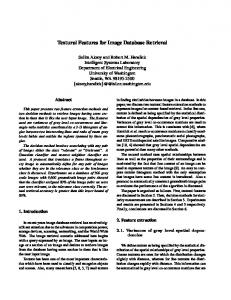
• Image 4 Image 5 Image 6 Figure 5: Three sample images (Image 4 - Image 6) Table 2: The user access patterns (usek,m) for Image 4 Image 6 q1 q2 q3
Image 4 1 0 1
Image 5 1 0 0
Image 6 0 1 1
…
…
…
…
… … … … …
Table 2 gives three example queries issued to our image database, where q1 is a user-issued query related to retrieving some images with parachute jumping scenes, and q2 and q3 are two other queries with their interests in natural scenes with sky, mountain and grass. It is worth mentioning that in our training process, the queries issued to each image category (landscape, flower, etc.) are almost the same because the query images are randomly selected by the training system from different image categories. By recording different users’ feedbacks during the training process, the corresponding access frequencies accessk for q1, q2, and q3 are 8, 7 and 1, respectively. In Table 2, the entry (k, m) = 1 indicates that the mth image is accessed by query qk. For example, Image 4 and Image 5 (as shown in Figure 5) are accessed together in q1 with their corresponding entries in the user access pattern matrix having value 1, and the access frequency access1 for q1 is 8. As for queries q2 and q3 that focus on retrieving natural scene images, access2 equals to 7 while access3 equals to 1. Notice that Image 4 and Image 6 are accessed together in q3 but not in q2, which is due to the different human perceptions (parachute jumping scene or landscape scene) on Image 4. However, since most of the users regard Image 4 as a parachute jumping scene rather than a landscape scene, the value of access1 is significantly larger than that of access3. Consequently, after the system training, Image 5 is more likely to be retrieved than Image 6, given Image 4 as the query image. Thus, the users’ subjective concepts about the images are captured by the pair of user access pattern and user access frequency.
2.2.2 Relative Affinity Matrix A Based on the information contained in the training data set, we can capture the affinity relationships among the images in the database. That is, the more frequently two images are accessed together, the more closely they are related to each other. The relative affinity matrix A is constructed in two steps as follows: •
Firstly, a matrix AF is defined to capture the affinity measurements among all the images using user access patterns and access frequencies as follows:
Definition 2: Each entry affm,n in matrix AF indicates how frequently two images m and n are accessed together, and consequently how closely these two image are related to each other, where
Then the matrix A can be obtained via normalizing AF per row and represents the relative affinity relationships among all the images in the database. Let am,n be the element in the (m, n) entry in A, where
a m, n =
aff m,n
∑n∈d aff m,n
(3)
For the sake of efficiency, instead of updating A matrix on-line, the training system only records all the user access patterns and access frequencies during a training period. Once the number of newly issued-queries reaches a threshold, the update of A matrix is triggered automatically. All the computations are done offline.
2.3 Retrieval Process Component After the training process, the low-level features and the highlevel concepts of the images in the database are connected more closely, and the system is ready for image retrieval. However, as we mentioned earlier, efficiency is an important issue in CBIR. The proposed content-based image retrieval framework solves this problem by conducting the retrieval process in two steps: 1.
A pre-filtering process is performed on the principal component subspace to reduce the search space.
2.
Perform the actual retrieval process that computes the similarity functions on the original feature space only for those candidate images.
2.3.1 Pre-Filtering Process The principal component analysis (PCA) [16] is integrated into our framework to generate a smaller feature space obtained by applying PCA on the original feature space (matrix B). The resulting principal components will form a more compact feature space for the purpose of pre-filtering. By reducing the search space in this manner, the number of images that need to perform exact similarity matching is reduced, which in turn reduces the computation time since exact similarity matching is more expensive in terms of computation.
2.3.1.1 Principal Component Analysis (PCA) The main capability of PCA is to reduce the dimensionality of the original feature space without losing the essential information [16]. Principal components are particular linear combinations of p features (X1, X2, …, Xp), which hold three important properties. First, principal components are uncorrelated. Second, the first principal component has the highest variance, while the second principal component has the second highest variance, and so on. Third, the total variation in all principal components combined is equal to the total variation in the original features X1, X2, …, Xp. Principal components can be easily obtained from the eigenanalysis of the covariance matrix or the correlation matrix of the original features. Principal components from these two matrices usually are not the same, and they are not simple functions of the others. It is better to perform PCA on the correlation matrix if the variables
are measured on scales with wildly different ranges or if the units of measurement are not commensurate [17]. Although it requires p principal components to reproduce the total system’s variability, often a small number k of the principal components are sufficient to explain the variability. In such cases, the initial p features can be replaced by the first k principal components, and the original data set (consisting of n measurements on p features) is reduced to a data set consisting of n measurements on k principal components. There will be almost as much information in the k components as there is in the original p features, if k is chosen appropriately.
2.3.1.2 Obtain Principal Components As mentioned earlier, the feature matrix B contains 12 color features and 9 spatial location features denoted by X1, X2, …, X21 that are normalized to lie in the range of 0.0 to 0.5. In this study, principal components are then obtained from the covariance matrix computed from B. Only the first two principal components that account for 50.12% of the total variation in the data are used as image pre-filtering, which can reduce the search space and lower the processing time. Though we sacrifice some of the information in the original feature space in an exchange for search efficiency, these two principal components seem adequate since they provide reasonably good retrieval results (as illustrated in the experimental results in Section 3).
2.3.1.3 Pre-Filtering to Reduce the Search Space Since the image retrieval process is usually computationally expensive in particular with a large number of features, the prefiltering step is needed to reduce the search space. The principal component scores for each image in the database are computed and stored together with the image. The idea for pre-filtering is to get all the images that have principal component scores close to those of the query image in the principal component subspace, while filtering out those images that are unlikely to be similar to the query image. For a large image database, the computation is very expensive. To achieve real time processing, we propose to use principal component scores 1 and 2 to construct a candidate image pool and only the images included in this candidate pool will require distance computations. Given a desired candidate pool size c (e.g., 100), the top c images that have principal component score 1 closest to that of the query image will be identified. Similarly, the top c images for principal component score 2 are also identified. The intersection of the two sets of images is the desired candidate image pool. If the size of the intersection set is less than c, then the scan scope in component scores 1 and 2 is increased until the candidate pool is filled. This simpler approach is reasonable due to the fact that principal components are uncorrelated and therefore the nearest neighbors found from individual principal component distributions will not be much different from the joint distribution.
2.3.2 Similarity Matching Process After the pre-filtering process, the size of the candidate image pool for a certain query can be reduced dramatically. Then the exact retrieval process can be carried out to extract the most matched images based on both the image features and the relative affinities among image learned from the training process. Let C be the total number of images in the candidate
image pool, p be the total number of distinct features of the images in the database, and the non-zero features of the query image q be denoted as {o1, o2, …, oT}, where T is the total number of non-zero features in the query (1≤T≤ p). Definition 3: Wt(i) is defined as the edge weight from the image i to the query image q at the evaluation of the tth feature (ot) in the query, where 1≤i≤C and 1≤t≤T. Based on the definition, the retrieval algorithm is given as follows. At t = 1,
W1 (i) = aq,i (1− | bi (o1 ) − bq (o1 ) | / bq (o1 ))
(4)
The values of Wt+1(i), where 1≤t≤T-1, are calculated by using the values of Wt(i).
Wt +1 (i) = Wt (i)(1− | bi (ot +1 ) − bq (ot +1 ) | / bq (ot +1 ))
(5)
Then the similarity function is defined as: S (i) =
T
∑
t =1
(6)
W t (i)
Here, aq,i (aq,i∈A) is the relative affinity relationship to indicate how closely the query image q is related to image i, and bi(ok) (bi(ok)∈B) is the value of the kth feature extracted from image i. The S(i) value for image i in the candidate image pool represents the similarity score between images q and i, where a larger score suggests the more similarity between images q and i. Input: query image, matrices A, B
Obtain first two principal component scores Pre-filtering process
Obtain feature vector {o1, o2…oT}
Get candidate image pool C t=1
t