Image Edge Detection Based on Gaussian Mixture Model in

Hindawi Publishing Corporation Journal of Electrical and Computer Engineering Volume 2016, Article ID 4125909, 10 pages http://dx.doi.org/10.1155/2016/4125909

Research Article Image Edge Detection Based on Gaussian Mixture Model in Nonsubsampled Contourlet Domain Li Yang,1 Chang Xia,2 and Chang Juan3 1

School of Computer Science and Engineering, Beifang University of Nationalities, Yinchuan 750021, China The Institute of Information and System Science, School of Mathematics and Information Science, Beifang University of Nationalities, Yinchuan 750021, China 3 Graduate School, Ningxia University, Yinchuan 750021, China 2

Correspondence should be addressed to Chang Xia; [email protected] Received 8 January 2016; Revised 31 May 2016; Accepted 29 June 2016 Academic Editor: Panajotis Agathoklis Copyright © 2016 Li Yang et al. This is an open access article distributed under the Creative Commons Attribution License, which permits unrestricted use, distribution, and reproduction in any medium, provided the original work is properly cited. In order to get accurate location and continuous edges, Gaussian mixture model and local direction modulus nonmaxima suppression are used in high frequency subbands of nonsubsampled Contourlet transform. The distribution of NSCT high frequency subbands coefficients has the “high spikes, long tail” non-Gaussian statistical characteristic. Gaussian mixture model (GMM) is used to distinguish the linear singular signal and the nonlinear singular signal on the high frequency subbands. Local direction modulus nonmaxima suppression is used to refine the linear singular signal. An appropriate threshold is used to distinguish edge pixels and nonedge pixels to get binary image. The experimental results demonstrate that the proposed method can capture more continuous edges in multiple directions and has accurate edge location. And the edges are with great convenience for the image recognition.

1. Introduction Image edge detection plays a very important role in image processing [1]. The results of image edge detection will directly affect the performance of image understanding, analysis, and recognition. The classical edge detectors based on gradient are concise and easy to understand, such as Sobel and Prewitt operators. Because of doing the average operation in these algorithms, they will lose some detailed information and make the edges blur. So the accuracy of location is not high. Canny edge detection usually gives good performance. Canny algorithm uses two different thresholds to detect strong edges and weak edges, respectively. Weak edges will be detected when weak edges are connected to strong edges. But weak edges will be ignored when weak edges are not connected to strong edges. Due to using Gaussian filter in the Canny edge detection method, some weak edges will be smoothed. And the detected edges obtained are more miscellaneous, so it is difficult to identify the main contours.

As the multiscale analysis is introduced, the image processing methods based on wavelet have obtained good results. Wavelet transform is famous for its time frequency localization, multiscale, and multiresolution. It is a very effective tool for image edge detection in image processing [2], such as the wavelet modulus maxima edge detection method. But the basis functions of wavelet transform are isotropic, so it cannot capture more directional information in images [3]. In the recent years, multiscale geometric analysis has grown constantly, and new methods based on the new multiscale transforms are proposed, such as the curvelet and Contourlet transform [4]. The Contourlet transform was proposed to address the lack of geometrical structure in the separable twodimensional wavelet transform. The research results show that the performance of the image edge detection based on the new multiscale transforms is better than those based on the wavelet transform. The Contourlet transform is a real 2D image representation using a directional filter and a Laplacian pyramid, which can effectively capture contours in an image

2

Journal of Electrical and Computer Engineering 𝜔2

(𝜋, 𝜋)

The low frequency subband

𝜔1

Original NSDFB image NSDFB (−𝜋, −𝜋) (a) Nonsubsampled directional filter bank

(b) Frequency resolution

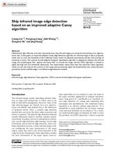
Figure 1: The structure of nonsubsampled Contourlet transform.

and can achieve better expression of image than the wavelet transform. It has the anisotropic characteristics. Because of the process of downsampling and upsampling, the Contourlet transform is shift-variance and always Gibbs phenomena around singularities. In 2006, the nonsubsampled Contourlet transform (NSCT) [5] was proposed by Cunha et al. The NSCT has better performance of the NSCT in image denoising and enhancement applications. NSCT is composed of the nonsubsampled pyramid filter and the nonsubsampled direction filter, so it is shift-invariance [6]. In this paper, a method of edge detection based on nonsubsampled Contourlet transform and Gaussian mixture model is proposed. The probability and statistics analysis is applied in the NSCT coefficients. The Gaussian mixture model is used to distinguish the linear singular signal and nonlinear singular signal on the high frequency subbands automatically. Local direction modulus nonmaxima suppression is used to refine the linear singular signal. An appropriate threshold is used to distinguish edge pixels and nonedge pixels to get binary image. We compare the proposed method with the classical Canny operator, Sobel operator, the wavelet method [2], and the method based on cellular neural network (CNN) [7]. The proposed method can capture more continuous edges in multiple directions and has accurate edge location.

2. Modeling NSCT High Frequency Coefficients 2.1. Nonsubsampled Contourlet Transform. NSCT consisted of the nonsubsampled pyramid filter banks (NSPFB) and the nonsubsampled directional filter banks (NSDFB) [6]. The two independent parts are shift-invariant. NSPFB is used for multiscale decomposition. NSDFB uses singular points of the same direction to synthesize the NSCT coefficients. NSDFB

is shown in Figure 1(a). Frequency resolution is shown in Figure 1(b). The distribution of NSCT high frequency subbands coefficients has the “high spikes, long tail” non-Gaussian statistical characteristic, as shown in Figure 2(a). High frequency subband coefficients consist of a few “big” coefficients and most “small” coefficients. The “small” coefficients contain less information and the “big” coefficients contain main information. Other high frequency directional subbands also have the similar distribution. Based on these characteristics to distinguish the linear singular signal and the nonlinear singular signal, Gaussian mixture model is used to model subbands, as shown in Figure 2(b); we use one Gaussian density function with big variance and one Gaussian density function with small variance to approximate the distribution. The “big” coefficients represent the linear singular signal. The linear singular signal is corresponding to the image edges. 2.2. Parameter Estimation of Gaussian Mixture Model. We model each high frequency directional subband through the Gaussian mixture model. 𝑥V,𝑤 is the coefficient which is in the V scale and the 𝑤 high frequency directional subband; 𝑁 V,𝑤 be in 𝑥V,𝑤 is the number of all coefficients in 𝑥V,𝑤 . Let 𝑥𝑚,𝑛 matrix, where 𝑚 is the column and 𝑛 is the row. Assume that V,𝑤 is independent of each other and obeys each sample in 𝑥𝑚,𝑛 V,𝑤 will be divided the 𝐾 Gaussian distribution [8], 𝐾 = 2. 𝑥𝑚,𝑛 into two classes: one class is “big” state; the other is “small” state. V,𝑤 is 𝑓V,𝑤 (𝑥) = Density function of 𝑥𝑚,𝑛 𝐾 𝐾 V,𝑤 V,𝑤 V,𝑤 V,𝑤 V,𝑤 V,𝑤 ∑𝑘=0 𝜋𝑘 𝑁 (𝑥𝑚,𝑛 | 𝜇𝑘 , Σ𝑘 ). There, ∑𝑘=0 𝜋𝑘 = 1, where 𝑘 = 0 or 1: 0 means “big” state and 1 means “small” state; 𝜇𝑘V,𝑤 is the 𝑘 class means; ΣV,𝑤 𝑘 is the 𝑘 class covariance, where V is the decomposition scale and 𝑤 is the filter direction. Expectation maximization algorithm can be used to calculate the optimal parameters of GMM by E-Step and MStep.

Journal of Electrical and Computer Engineering

3

250

0.7

0.6

200

0.5 150

0.4 0.3

100

0.2 50

0.1

0 −50

−25

0

25

−50

(a) “High spikes, long tail” non-Gaussian statistical characteristic

0 −30

−20

−10

0

−10

−20

−30

(b) The two classes of the coefficients

Figure 2: Statistics of the image NSCT coefficients.

V,𝑤 Input: high-frequency directional sub-bands 𝑥𝑚,𝑛 V,𝑤 (1) Employ (1)∼(3) to calculate the probability of 𝑥𝑚,𝑛 generated by each component (2) Employ (4)∼(7) to calculate the 𝑢𝑘V,𝑤 , 𝜋𝑘V,𝑤 , 𝑁𝑘V,𝑤 (3) Repeated iteration, until the values of the likelihood function achieves convergence. V,𝑤 , 𝑢𝑘V,𝑤 , (4) Calculate the probability of 𝑥𝑖 generated by each component according to 𝑥𝑚,𝑛 V,𝑤 generated by the “big” variance of Gaussian 𝜋𝑘V,𝑤 , 𝑁𝑘V,𝑤 . Let pro0 be the probability of 𝑥𝑚,𝑛 V,𝑤 generated by the “small” variance of Gaussian model; let pro1 be the probability of 𝑥𝑚,𝑛 model. V,𝑤 (5) If pro0 < pro1, set 0 to 𝑥𝑚,𝑛 V,𝑤 V,𝑤 Output: 𝑥𝑚,𝑛 (new high-frequency directional sub-bands 𝑥𝑚,𝑛 )

Algorithm 1: Data screening algorithm by Gaussian mixture model.

V,𝑤 E-Step: calculating the probability of 𝑥𝑚,𝑛 generated by each component

𝛾V,𝑤 (𝑖, 𝑘) =

V,𝑤 𝜋𝑘V,𝑤 𝑁 (𝑥𝑚,𝑛 | 𝜇𝑘V,𝑤 , ΣV,𝑤 𝑘 ) V,𝑤 V,𝑤 V,𝑤 V,𝑤 ∑𝐾 𝑗=0 𝜋𝑗 𝑁 (𝑥𝑚,𝑛 | 𝜇𝑗 , Σ𝑗 )

.

(1)

V,𝑤 and 𝜋𝑘V,𝑤 is In formula (1), 𝛾V,𝑤 (𝑖, 𝑘) is the probability of 𝑥𝑚,𝑛 the weighting factor. M-Step: calculating 𝑁𝑘V,𝑤 , 𝑢𝑘V,𝑤 , and 𝜋𝑘V,𝑤 , iteratively 𝑁

𝑁𝑘V,𝑤 = ∑𝛾V,𝑤 (𝑖, 𝑘) ,

(2)

𝑖=1

nonmaxima suppression to refine the linear signal. High frequency directional subbands contain the directional information, so there is no need to calculate the direction of the modulus; just compare the modulus of pixel and the modulus of the two gradient directional pixels of this pixel [9]. Determine whether it is a local maximum modulus and retain if it is. For example, there are eight directions in some new high frequency directional subbands. So there are eight sectors, which are 𝜋/16, 3𝜋/16, 5𝜋/16, 7𝜋/16, 9𝜋/16, 11𝜋/16, 13𝜋/16, V,𝑤 V,𝑤 ) is the modulus of 𝑥𝑚,𝑛 . argV,𝑤 is and 15𝜋/16. Mod (𝑥𝑚,𝑛 V,𝑤 the equivalent gradient of 𝑥 . Figure 3 is the directional subband equivalent gradient.

𝑢𝑘V,𝑤 =

1 𝑁 V,𝑤 V,𝑤 , ∑𝛾 (𝑖, 𝑘) 𝑥𝑚,𝑛 𝑁𝑘V,𝑤 𝑖=1

(3)

2.5. Algorithm 2: Local Mold Maxima Suppression Algorithm. See Algorithm 2.

𝜋𝑘V,𝑤 =

𝑁𝑘V,𝑤 . 𝑁

(4)

2.6. Our Proposed Edge Detection Algorithm. The proposed edge detection algorithm is summarized as follows:

2.3. Algorithm 1: Data Screening Algorithm by Gaussian Mixture Model. See Algorithm 1. 2.4. Local Direction Modulus Nonmaxima Suppression. After executing Algorithm 1, we use local direction modulus

Input: original image. Step 1. Decompose the original image into high frequency V,𝑤 and low frequency subband by directional subbands 𝑥𝑚,𝑛 NSCT.

4

Journal of Electrical and Computer Engineering V,𝑤 Input: new high-frequency directional sub-bands 𝑥𝑚,𝑛 If 3𝜋/16 < argV,𝑤 < 5𝜋/16 ‖ 11𝜋/16 < argV,𝑤 < 13𝜋/16 V,𝑤 V,𝑤 V,𝑤 V,𝑤 ) < mod(𝑥𝑚,𝑛−1 ) ‖ mod(𝑥𝑚,𝑛 ) < mod(𝑥𝑚,𝑛+1 ) If mod(𝑥𝑚,𝑛 V,𝑤 𝑥𝑚,𝑛 = 0; End End ElseIf 𝜋/16 < argV,𝑤 < 3𝜋/16 ‖ 9𝜋/16 < argV,𝑤 < 11𝜋/16 V,𝑤 V,𝑤 V,𝑤 V,𝑤 ) < mod(𝑥𝑚−1,𝑛+1 ) ‖ mod(𝑥𝑚,𝑛 ) < mod(𝑥𝑚+1,𝑛−1 ) If mod(𝑥𝑚,𝑛 V,𝑤 𝑥𝑚,𝑛 = 0; End End ElseIf 5𝜋/16 < argV,𝑤 < 7𝜋/16 ‖ 13𝜋/16 < argV,𝑤 < 15𝜋/16 V,𝑤 V,𝑤 V,𝑤 V,𝑤 ) < mod(𝑥𝑚−1,𝑛 ) ‖ mod(𝑥𝑚,𝑛 ) < mod(𝑥𝑚+1,𝑛 ) If mod(𝑥𝑚,𝑛 V,𝑤 𝑥𝑚,𝑛 = 0; End End Else V,𝑤 V,𝑤 V,𝑤 V,𝑤 ) < mod(𝑥𝑚−1,𝑛 ) ‖ mod(𝑥𝑚,𝑛 ) < mod(𝑥𝑚+1,𝑛 ) If mod(𝑥𝑚,𝑛 V,𝑤 = 0; 𝑥𝑚,𝑛 End End V,𝑤 V,𝑤 (new high-frequency directional sub-bands 𝑥𝑚,𝑛 ) Output: 𝑥𝑚,𝑛

Algorithm 2: Local mold maxima suppression algorithm.

3𝜋/16

5𝜋/16

7𝜋/16

3

2

1

𝜋/16

Output: edge detection result.

0

4 9𝜋/16

them. Set threshold to distinguish edge pixels and nonedge pixels to get binary image.

3. Experimental Results

5

6 11𝜋/16

7

15𝜋/16

13𝜋/16

Figure 3: Directional subband equivalent gradient.

In order to quantify the performance of the proposed method, FOM (Pratt’s Figure of Merit) [10] is used to compare the performance of edge detection methods, because the edges of the standard image must be obtained while using FOM. Because of this, we can just use the synthetic images. The FOM is computed as follows: 𝑁

Step 2. Let low frequency subband coefficients be 0. V,𝑤 V,𝑤 Step 3. Employ Algorithm 1 to process 𝑥𝑚,𝑛 , we get new 𝑥𝑚,𝑛 , V,𝑤 and new 𝑥𝑚,𝑛 are the linear singular signal here. V,𝑤 Step 4. Employ Algorithm 2 to process 𝑥𝑚,𝑛 , which is got by V,𝑤 V,𝑤 Step 3, we get new 𝑥𝑚,𝑛 , and new 𝑥𝑚,𝑛 are the linear singular signal refined here.

Step 5. Reconstruct image using high frequency coefficients V,𝑤 processed by Step 3 and low frequency coefficients 𝑥𝑚,𝑛 processed by Step 1. Step 6. After NSCT inverse transform, there will be a data matrix. There will be two types of data in that matrix, the modulus of one type is big, and the modulus of the other type is small. An appropriate threshold can be easily set to separate

FOM =

𝐴 1 1 , ∑ max {𝑁𝐼 , 𝑁𝐴} 𝑖=1 1 + 𝛼𝑑𝑖

(5)

where 𝑁𝐼 and 𝑁𝐴 are the number of ideal and detected edge pixels, respectively, the parameter 𝛼 is a constant, and 𝑑𝑖 is the vertical distance between an actual edge pixel and the nearest ideal edge pixel. The FOM measures the accuracy of localization. The more the FOM is, the more the quality of the edge detection is. In order to objectively discuss the accuracy of the localization, the false edge pixels are not covered while computing the FOM. A synthetic image is used to calculate FOM. The proposed method, CNN, Canny, Sobel operators, NSCT, and the wavelet method are used to detect the edge of the synthetic image. The NSCT method is used to detect edges without using GMM. Figure 4 shows the results detected by the different methods. Table 1 shows the FOM calculations by


5

(a)

(b)

(c)

(d)

(e)

(f)

(g)

Figure 4: The results of the edge detection: (a) the synthetic image, (b) the proposed method, (c) the method based on CNN, (d) Canny operator, (e) Sobel operator, (f) wavelet method, and (g) NSCT method. Table 1: The FOM calculations with different methods. Figure 4 FOM

The proposed method

The method based on CNN

Canny operator

Sobel operator

NSCT

Wavelet method

0.9631

0.8934

0.8256

0.7937

0.6432

0.7231

different methods. The results demonstrate that the accuracy of the localization of the proposed method is more accurate than Canny operator, Sobel operator, wavelet method, NSCT method, and the method based on CNN. The accuracy of the localization of the proposed method is the best. Because of

not using GMM to distinguish the linear singular signal and the nonlinear singular signal on the high frequency subbands, the edges detected by the NSCT method are interrupted by the nonlinear singular signal. So the accuracy of the localization of the NSCT method is very low. The Canny,

6


(a)

(b)

(c)

(d)

(e)

(f)

(g)

Figure 5: Edge detection results: (a) original image; (b) the result by Canny; (c) the result by our method; (d) the result by Sobel; (e) the result by wavelet method; (f) the method based on CNN; (g) NSCT method.

Sobel operators, and CNN method are sensitive to noise, so their accuracy of the localization is lower than the proposed method. Three standard images, which are Barbara (size 256 ∗ 256), Lenna (size 256 ∗ 256), and boat (size 512 ∗ 512), are used to test in the experiments. We select “9-7” pyramid decomposition and “pkva” directional filter bank for NSCT decomposition. Decomposition level is 3 and each level has eight high frequency directions. Experimental results are shown in Figures 5, 6, and 7.

The linear singular edges of the table cloth detected in Figure 5(b) are clearer than those in Figures 5(c), 5(d), 5(e), and 5(f). The texture edges of the tassels in Figure 6(b) are more continuous than those in Figures 6(c), 6(d), 6(e), and 6(f). Contour edges detected of the hull in Figure 7(b) are more complete than those in Figures 7(c), 7(d), and 7(f). The edges are too miscellaneous to distinguish the main contours in Figures 5(c), 6(c), 7(c), 5(d), 6(d), and 7(d). Because the wavelet just has two directions, it cannot capture more directional details. Because of not using GMM to distinguish


7

(a)

(b)

(c)

(d)

(e)

(f)

(g)


the linear singular signal and the nonlinear singular signal on the high frequency subbands, the edges detected by the NSCT method are interrupted by the nonlinear singular signal. From Figures 5(g), 6(g), and 7(g), we also cannot distinguish the main contours. Because the NSCT has good directionality, anisotropy, and decorrelation, the proposed method can capture more directional details. And the proposed method can capture the main contours because of using the GMM. From Figures 5(b), 6(b), and 7(b), we can clearly see the main contours in the images. In order to evaluate the algorithm, the quantitative analysis is adopted [11]. In Table 2, CEN denotes the number

of continuous edge pixels in edge image. TEN represents the number of all pixels in edge image. 𝑅 denotes the ratio of TEN to CEN. The more 𝑅 is, the more image edge is continuous. 𝑅 is computed as follows: TEN (6) . CEN Table 2 shows that the edges obtained by the proposed method are more continuous than other methods. Because the wavelet just has two directions, it cannot capture more directional details. Though the NSCT method can capture more edges than the Canny and Sobel operators, the pixels 𝑅=

8


(a)

(b)

(c)

(d)

(e)

(f)

(g)


detected by the NSCT method contain so much the nonlinear singular signal. The proposed method can capture more details than other methods. MSE (Mean Squared Error) is a standard to measure the accuracy of localization. Generally, when MSE is greater, the accuracy of localization is less. When MSE is less, the accuracy of localization is higher. The MSE is computed as follows: MSE =

1 𝑚−1 𝑛−1 󵄨󵄨 󵄨2 ∑ ∑ 󵄨𝐼 (𝑖, 𝑗) − 𝐾 (𝑖, 𝑗)󵄨󵄨󵄨 . 𝑚𝑛 𝑖=0 𝑗=0 󵄨

(7)

Table 3 shows the MSE results of different methods. We can see that the proposed method has a lower MSE than other methods. It means that the proposed method has high accuracy of localization. Because of not using GMM to distinguish the linear singular signal and the nonlinear singular signal on the high frequency subbands, the edges detected by the NSCT method are interrupted by the nonlinear singular signal. So the accuracy of localization is low in the NSCT method. The results show that, compared with traditional edge detection methods, the proposed method possessed better edge locating ability and keeps more edge details.


9

Table 2: The comparison of the different detection methods. Image

Detection method Canny Our method Sobel Wavelet CNN NSCT Canny Our method Sobel Wavelet CNN NSCT Canny Our method Sobel Wavelet CNN NSCT

Barbara

Lenna

Boat

CEN 9896 16113 8646 7556 12703 21822 7935 8462 6731 5470 4544 23823 32011 56781 34536 25920 18805 80251

TEN 8713 14984 7163 6388 10793 19790 7184 7924 5831 4822 3627 22043 29030 54791 30172 23479 13647 73809

𝑅 0.8805 0.9299 0.82848 0.8454 0.8496 0.9069 0.9041 0.9364 0.86629 0.8815 0.7982 0.9253 0.9069 0.965 0.87364 0.9058 0.7257 0.9197

Table 3: MSE of the different detection methods. Image Barbara Boat Lenna

Sobel MSE

Canny MSE

CNN MSE

NSCT

Wavelet MSE

Proposed method MSE

0.64891 0.5945 0.84657

0.4351 0.3946 0.5874

0.2574 0.2415 0.4059

0.7859 0.6845 0.7548

0.5874 0.6842 0.3897

0.1989 0.1826 0.2834

4. Conclusions We have presented an edge detection method based on nonsubsampled Contourlet transform and Gaussian mixture model. The proposed method is based on nonsubsampled Contourlet transform and Gaussian mixture model. It can capture more directional information and continuous edges. It overcomes the shortage of the limited directions of wavelet transform. The main contours in the image can be clearly expressed. This method can effectively locate the edge. The thick edges detected by the proposed method express the main edges in the images, which are with great convenience for the image recognition. The proposed method runs slowly; it needs to be improved in the future.

Competing Interests The authors declare that they have no competing interests.

Acknowledgments This work is supported by the National Natural Science Foundation of China (Grant no. 61440044, no. 61561001, no. 61102008, no. 61163017, no. 61261043, and no. 61462002), the

Ningxia Science Foundation of China (Grant no. NZ13097), and the Foundations of Research Projects of State Ethnic Affairs Commission of P. R. China (Grant no. 14BFZ003).

References [1] S. Bhattacharya, “Edge detection in range images using nonlinear laplacian operators,” IETE Journal of Research, vol. 48, no. 3-4, pp. 205–209, 2002. [2] H. Zhang, L. Luo, K. Yang, L. Wang, and X. Gao, “Improved multi-scale wavelet in pantograph slide edge detection,” Optik, vol. 125, no. 19, pp. 5681–5683, 2014. [3] M. T. Alonso, C. L´opez-Mart´ınez, J. J. Mallorqu´ı, and P. Salembier, “Edge enhancement algorithm based on the wavelet transform for automatic edge detection in SAR images,” IEEE Transactions on Geoscience & Remote Sensing, vol. 49, no. 1, pp. 222– 235, 2011. [4] M. N. Do and M. Vetterli, “The contourlet transform: an efficient directional multiresolution image representation,” IEEE Transactions on Image Processing, vol. 14, no. 12, pp. 2091–2106, 2005. [5] A. L. D. Cunha, J. Zhou, and M. N. Do, “Nonsubsampled contourlet transform: theory, design, and applications,” IEEE Transactions on Image Processing, vol. 15, no. 10, pp. 3089–3101, 2006.

10 [6] L. Xu, J. Du, and Q. Li, “Image fusion based on nonsubsampled contourlet transform and saliency-motivated pulse coupled neural networks,” Mathematical Problems in Engineering, vol. 2013, Article ID 135182, 10 pages, 2013. [7] S. Deng, Y. Tian, X. Hu, P. Wei, and M. Qin, “Application of new advanced CNN structure with adaptive thresholds to color edge detection,” Communications in Nonlinear Science and Numerical Simulation, vol. 17, no. 4, pp. 1637–1648, 2012. [8] X. Chang, L. Jiao, F. Liu, and Y. Sha, “SAR image despeckling using scale mixtures of gaussians in the nonsubsampled contourlet domain,” Chinese Journal of Electronics, vol. 24, no. 1, pp. 205–211, 2015. [9] T. Y. Lo, K. S. Sim, C. P. Tso, and M. E. Nia, “Improvement to the scanning electron microscope image adaptive canny optimization colorization by pseudo-mapping,” Scanning, vol. 36, no. 5, pp. 530–539, 2014. [10] I. E. Abdou and W. K. Pratt, “Quantitative design and evaluation of enhancement/thresholding edge detectors,” Proceedings of the IEEE, vol. 67, no. 5, pp. 753–763, 1979. [11] G.-Y. Zhang, G.-Z. Gong, and W.-L. Zhu, “A novel method of color image edge detection based on cloning algorithm,” Acta Electronica Sinica, vol. 34, no. 4, pp. 702–707, 2006.


International Journal of

Rotating Machinery

Engineering Journal of

Hindawi Publishing Corporation http://www.hindawi.com

Volume 2014

The Scientific World Journal Hindawi Publishing Corporation http://www.hindawi.com

Volume 2014


Distributed Sensor Networks

Journal of

Sensors Hindawi Publishing Corporation http://www.hindawi.com

Volume 2014


Volume 2014


Volume 2014

Journal of

Control Science and Engineering

Advances in

Civil Engineering Hindawi Publishing Corporation http://www.hindawi.com


Volume 2014

Volume 2014

Submit your manuscripts at http://www.hindawi.com Journal of

Journal of

Electrical and Computer Engineering

Robotics Hindawi Publishing Corporation http://www.hindawi.com


Volume 2014

Volume 2014

VLSI Design Advances in OptoElectronics


Navigation and Observation Hindawi Publishing Corporation http://www.hindawi.com

Volume 2014



Chemical Engineering Hindawi Publishing Corporation http://www.hindawi.com

Volume 2014

Volume 2014

Active and Passive Electronic Components

Antennas and Propagation Hindawi Publishing Corporation http://www.hindawi.com

Aerospace Engineering


Volume 2014


Volume 2014

Volume 2014




Modelling & Simulation in Engineering

Volume 2014


Volume 2014

Shock and Vibration Hindawi Publishing Corporation http://www.hindawi.com

Volume 2014

Advances in

Acoustics and Vibration Hindawi Publishing Corporation http://www.hindawi.com

Volume 2014