Image Encryption using the Two-dimensional Logistic Chaotic Map Yue Wua , Gelan Yangb∗ , Huixia Jinb and Joseph P. Noonana a Department
of Electrical and Computer Engineering, Tufts University
Medford, Massachusetts 02155, United States b Department
of Computer Science, Hunan City University Yiyang, Hunan 413000, China
∗ Email:
[email protected]
Abstract Chaos maps and chaotic systems have been proved to be useful and effective for cryptography. In this paper, the two-dimensional logistic map with complicated basin structures and attractors are first used for image encryption. The proposed method adopts the classic framework of the permutation-substitution network in cryptography and thus ensures both confusion and diffusion properties for a secure cipher. The proposed method is able to encrypt an intelligible image into random-like from the statistical point of view and the human visual system point of view. Extensive simulation results using test images from the USC-SIPI image database demonstrate the effectiveness and robustness of the proposed method. Security analysis results of using both the conventional and the most recent tests show that the encryption quality of the proposed method reaches or excels the current state-of-the-arts. Similar encryption ideas can be applied to digital data in other formats, e.g. digital audio and video. We also publish the cipher MATLAB open-source code under the web page https://sites.google.com/site/tuftsyuewu/source-code.
1
1
Introduction
Image security attracts extensive concerns from the public and the government in recent years. Unexpected exposure of private photos and divulged military and governmental classified images emphasizes the importance of the image security again and again. With the fast development of digital storages, computers and the world wide network, a digital image can be easily copied to mobile storage or transferred to the other side of the world within a second. However, such convenience could also be used by malicious/unauthorized users to rapidly spread the image information that it may cause uncountable losses for the owner(s) of images. Among various image security technologies, the image encryption is a straight-forward one with concerns in encrypting an image to an unrecognized and unintelligent one [1], where the source image and the encrypted image are called plaintext image and ciphertext image [2], respectively. One common approach of image encryption is to treat the image data the same as the one-dimensional binary bit stream, which extracts a plaintext image bit by bit and then encrypts this binary bit stream. The advantage of this approach is able to encrypt a digital image using the existing block/stream ciphers designed originally for binary bit streams. These ciphers include the well known ciphers/standards: the Digital Encryption Standard (DES) [3], the Advanced Encryption Standard (AES) [4], the TwoFish cipher [5] and the BlowFish cipher [6]. However, the tradeoff of using the one-dimensional bit stream/block based ciphers for image encryption is to sacrifice the two-dimensional nature of the image data [1]. Meanwhile, this type of image encryption is also inefficient in the sense of the extremely long bit stream extracted from the image data, which might be composed of more than a hundred thousand of pixels with 8 or 16 bits representation for each pixel [1]. Further, the stream/block size of the cipher is relatively small comparing to a common image size and thus the encryption is commonly performed over pixel blocks with high information redundancy. As a result, the encryption quality is poor in some reports [7]. In the research of image encryption algorithms/ciphers, efforts are found in two groups: optical image encryption, and digital image encryption. The former group adopts optics or optical instruments to build physical systems for image encryption [8, 9, 10, 11, 12] , which commonly relies on optics to randomize frequency components in an image. The later
2
group commonly takes advantages of an digital image and encrypts it either by an encryption algorithm in the form of software or a physical electronic device in the form of hardware. Among various digital image encryption methods, the chaos-based image encryption method is a family of methods that are believed good for encryption purposes. Because a chaotic system has high sensitivities to its initial values, high sensitivities to its parameter(s), the mixing property and the ergodicity [1, 13, 14], it is considered as a good candidate for cryptography. Since 1997, Fridrich applied chaos to encryption of digital images for the first time [15], chaos-based image encryption methods are researched for years [13, 16, 17, 18, 19, 20, 21, 22]. Some of these methods [13, 22] are flawed in treating pixel bytes still in the form of the bit stream and thus inefficient. Some are criticized for the weak keys, the limited key space, the vulnerability to selected plaintext/ciphertext attacks and other issues in [23, 24, 25]. In this paper, we adopt the two-dimensional Logistic map for image encryption in the first time with careful considerations for the diffusion and confusion properties [26] and possible attacks as well. This chaotic map is researched with respect to its mathematical properties and physical dynamics previously and it has been showed that this coupled logistic map for two dimensions has more complicated chaotic behaviors like basin structures and attractors [27]. We utilize this more complicated chaotic map to generate pseudo random sequences where we propose a key schedule algorithm to translate a binary encryption key to initial values and parameters used in the 2D logistic map. We develop an image encryption algorithm using these pseudo-random sequences under the framework of the permutationsubstitution network [2], which is proven to be very effective to provide both confusion and diffusion properties in stream ciphers and block ciphers [3, 4]. Simulation results of using the open-accessed USC-SIPI image database support the effectiveness and robustness of the proposed cipher for various images of contents and types. Finally, security analysis of using both the conventional quantitative measurements and the most recent qualitative measurements [7, 28] demonstrate that the proposed cipher is able to generated statistically random-like encrypted images. The reminder of the paper is organized as follows: Section 2 gives brief background information about the two-dimensional logistic map; Section 3 first gives the flowchart of the cipher and then discusses encryption stages consecutively; Section 4 shows the simulation 3
results and security analysis of the encrypted images using the proposed method; and Section 5 concludes this paper.
2
The Two-dimensional Logistic Map
The two-dimensional logistic map is researched for its complicated behaviors of the evolution of basins and attractors [27]. It has more complex chaotic behaviors than one-dimensional Logistic map.
2.1
Mathematical Definition
Mathematically, this 2D logistic map can be discretely defined as Eq. (1), where r is the system parameter and (xi , yi ) is the pair-wise point at the ith iteration. xi+1 = r(3yi + 1)xi (1 − xi ) 2D Logistic map:
y
i+1
(1)
= r(3xi+1 + 1)yi (1 − yi )
Fig. 1 shows the scatter plot of 30, 000 points from the trajectory [29] of the 2D logistic map using the parameter r = 1.19 and the initial value (x0 , y0 ) at (0.8909, 0.3342). Therefore, the ith point on the trajectory can be determined by knowing (x0 , y0 , r, i) as Eq. (2) shows. xi = L2D (x0 , y0 , r, i) x (2) y = L2D (x , y , r, i) i 0 0 y
2.2
Phase Portrait and Chaotic Behaviors
The 2D logistic map defined in Eq. (1) is a complex dynamical system. According to the value of the system parameter r, the map evolves from one kind of dynamics to another. More specifically, the behaviors of the map can be concluded as follows [27]: • When r ∈ (−1, 1), the system has one attractive node and two saddle points, and makes both x and y axes being unstable manifolds. • When r = 1, the attractive focus undergoes a Neimark-Hopf bifurcation [29]. 4
1
1
(xi,yi) Trajectory
0.9
(x0,y0) Initial value
0.8
0.8
0.6
0.7
0.4
0.6
0.2
0.5
0
0.4
−0.2
0.3
−0.4
0.2
−0.6
0.1
−0.8
0
0
0.2
0.4
0.6
0.8
−1 −1
1
−0.5
0
0.5
1
Figure 1: A trajectory of 2D logistic map. Figure 2: A phase portrait of 2D logistic map. • When r ∈ (1, 1.11), the attractive focus becomes repulsive and oscillations appears. • When r ∈ [1.11, 1.19], an alternation between existence of invariant close curve with oscillations, frequency locking, cyclic chaotic behaviors, contact bifurcations with basin boundaries and single chaotic attractor. • When r > 1.19, the system becomes unstable. Fig. 2 shows the phase portrait [29] of the 2D logistic map when r = 1.19. It is noticeable that this phase portrait matches the mathematical depiction of the 2D logistic map for r = 1.19. Since a (x, y) trajectory with respect to the chaotic behavior is random-like but is completely predictable when r and (x0 , y0 ) are both known, it can be used as a pseudo number generator for cryptography.
2.3
Complexity
The 2D logistic map defined in Eq. (1) has a higher complexity compared to the conventional logistic map[29], i.e. 1D logistic map defined in Eq. (3), where r is the parameter controlling the chaotic behaviors. Fig. 3 shows the bifurcation diagram [29] of the 1D logistic map, where
5
horizontal axis denotes the parameter r and vertical axis denotes x and each trajectory of the 1D logistic map about x with a fixed x is plotted as dots on the figure. 1D Logistic map: xi+1 = rxi (1 − xi )
(3)
Figure 3: The bifurcation diagram of the 1D logistic map. Quantitatively, the complexities of the 1D and 2D logistic maps and the Henon map [29] (see Eq. (4)) can be measured by using various means. Table 1 shows the complexity comparisons between these chaotic maps using Information Entropy [30], Lyapunov Exponent [31, 32], and Lyapunov Dimension [33, 34] with respect to different pairs of initial values. As seen from this table, the 2D logistic map has a higher information entropy scores than 1D logistic map, which implies that its trajectory is more random-like. Meanwhile, the 2D logistic map also has a larger Lyapunov exponent than the 1D logistic map, which implies that the 2D logistic map is more dynamic. Furthermore, the 2D logistic map even has a greater Lyapunov dimensions than the Henon map, a typical 2D chaotic map.
Henon Map:
xi+1 = yi + 1 − ax2 i y
i+1
6
= bxi
(4)
Table 1: Chaotic map complexity analysis 1D Logistic (r) Parameters Measurement\Comments Information Entropy1
Henon(a, b)
2D Logistic (r)
3.57
4.00
(1.40, 0.3)
1.11
1.19
Start of Chaos
End of Chaos
Chaos
Start of Chaos
End of Chaos
#Bins
H(x)
H(x)
H(x)
H(y)
H(x)
H(y)
H(x)
H(y)
256
4.8115
7.6895
7.8155
7.8155
6.2605
6.5547
7.8944
7.8938
512
5.2735
8.6773
8.8041
8.8041
7.1858
7.4551
8.8906
8.8900
λ1
λ1
λ1
λ2
λ1
λ2
λ1
λ2
Lyapunov Exponent2
0.0012
0.0693
0.4241
-1.6281
0.3646
-0.1166
0.5654
-0.2108
Lyapunov Dimension3
N \a
N \a
3
1.2605
4.1287
3.6824
Image Encryption using the 2D Logistic Map
Although the 2D logistic map has various behaviors according to different system parameters, in the paper we concentrate on the parameter interval r ∈ [1.1, 1.19], where the system is chaotic. Fig. 4 shows the flowchart of the proposed image encryption method using the 2D logistic map. And the internal loop is composed of 2D Logistic Permutation, 2D Logistic Diffusion and 2D Logistic Transposition where each stage itself is an image cipher and they together form the permutation-substitution network[2]. Detailed discussions about these stages are given in the next section. Similar to the encryption procedure, the decryption procedure is nothing but reverse the order of processing using the decryption key as Fig. 5 shows. In short, the encryption process can be written as C = Enc(P, K), and the decryption process is P = Dec(C, K).
3.1
Key Schedule and 2D Logistic Sequence Generator
We define our encryption key K as a 256-bit string composed of five parts x0 , y0 , r,T , and A1 · · · A8 as shown in Fig. 6, where (x0 , y0 ) and r are the initial value and the parameter 1
Information Entropy is measured over the discrete probability density function defined on #Bins on the
range of a chaotic map. 2 Lyapunov Exponent is measured with respect to each eigenvalue by using the Lyapunov toolbox under MATLAB. 3 Lyapunov Dimesnions is calculated by using the Lyapunov toolbox under MATLAB (Link: http:// www.mathworks.com/matlabcentral/fileexchange/233).
7
Figure 4: The flowchart of image encryption using the 2D logistic map.
Figure 5: The flowchart of image decryption using the 2D logistic map. in the 2D logistic map defined in Eq. (1), and A and T are the parameters of the linear congruential generator [35].
Figure 6: Key composition. Specifically speaking, we calculate a fraction value v from a 52-bit string {b−1 , b−2 , · · · , b−52 } using the IEEE 754 double-precision binary floating-point format for the fraction part as shown in Eq. (5) v=
52 X
b−i 2−i
(5)
i=1
Consequently, x0 , y0 , r and T can be found. For coefficients A0 , A1 , · · · , A7 , each of which is composed of 6-bit string {b0 , b1 , · · · , b5 }, we translate these 6-bit strings to integers and obtain the required coefficients. The initial value (xround# , y0round# ) for each round then can 0 8
be defined by the following equation: xround# = T + x0 A(round# mod 8)+1 mod 1 0 y round# = T + y A 0 (round# mod 8)+1 mod 1 0
(6)
, y0round# ) and r to generate a sufficiently As a result, we can use the initial value (xround# 0 long chaotic sequence, whose length equals to the number of pixels in the plaintext image P using Eq.(1). In such a way, we make encryption key K to control the pseudo random sequences from the 2D logistic map for each round.
3.2
2D Logistic Permutation
Without loss of generality, assume the size of the plaintext image P is M × N . Therefore, the total number of pixels in P is M N . Consider the initial value used in a round is (x0 , y0 ). A sequence of pair-wise x and y of length M N (exclude the initial value) can be generated via the 2D logistic map using Eq. (1). Let Xseq and Yseq be the x coordinate sequence and the y coordinate sequence of the 2D logistic map, respectively, as Eq. (7) shows. Xseq = {x1 , x2 , · · · , xM N }
(7)
Y = {y , y , · · · , y } seq 1 2 MN Rearrange elements of Xseq and Yseq whose number is M × N in the matrix form and obtain M ×N matrices X and Y , respectively. Then the rth row of X can be used to form a bijective mapping [2] eπx as shown in Eq. (8). Similarly, there also exists a bijection eπy between the cth column of Y and its sorted version Y sorted . sorted Xr,i = Xr,eπx (i)
(8)
sorted Yi,c = Xeπy (i),c
(9)
Consequently, the row permutation matrix U x and the column permutation matrix U y can be obtained via Eqs. (10) and (11), respectively. It can be easily verified that each row in U x is a permutation of the nature number sequence of {1, 2, · · · , N }. In the same manner, each column in U y is a permutation of the nature number sequence of {1, 2, · · · , M }. r=2 r=M 0 U x = [er=1 πx , eπx , · · · , eπx ]
9
(10)
c=2 c=N U y = [ec=1 πy , eπy , · · · , eπy ]
(11)
Finally, the 2D logistic permutation is defined as Algorithm 1 by using the row permutations and column permutations of Eqs. (10) and (11). Fig. 7 shows the intermediate results of the 2D logistic permutation described in Algorithm 1. It is noticeable that after the 2D logistic permutation, the pixels in the plaintext image P have been well shuffled and the permutated image C perm is unrecognizable. Algorithm 1 2D Logistic Permutation Algorithm Input: 2D plaintext image P , row permutation matrix U x and column permutation matrix U y Output: Ciphertext image C for r = 1 : M do for c = 1 : N do x ,c ;(Pixel permutation along x) Qr,c = PUr,c
end for end for for r = 1 : M do for c = 1 : N do y ;(Pixel permutation along y) Cr,c = Qr,Ur,c
end for end for
Figure 7: 2D logistic permutation results. (a) plaintext image P ; (b) ciphertext image Q of row shuffling; (c) ciphertext image C of row and column shuffling.
10
3.3
2D Logistic Diffusion
In order achieve good diffusion properties [26], we apply the logistic diffusion for every S × S image block Pb within the plaintext image P over the finite field GF (28 ) as shown in Eq. (12), where S is the block size variable determined by the plaintext image format, and Ld is the maximum distance separation matrix [4] found from 4 × 4 random permutation matrices defined in Eq. (14). Cb = (Ld · Pb · Ld )28
4 2 1 3 Ld = 2 4 3 1
1 4 3 2
−1 Pb = (L−1 d · Cb · Ld )28 3 71 216 173 117 173 117 71 216 2 and (L−1 d )28 = 216 71 117 173 1 4 117 173 216 71
(12) (13)
(14)
It worthwhile to note that if the plaintext image P is of 8-bit grayscale or RGB color types, both of which code an image pixel as a byte (1 byte = 8 bits), then the image block Pb is of size 4 × 4; while if the plaintext image is a binary image, then Pb is of size 32 × 32 in bits (equivalent to a 4 × 4 image block in bytes). In the case that the plaintext image P with a size M × N which is not dividable by S, the processing block size of Pb , we then only apply this process with respect to the region SbM/Sc × SbN/Sc and b.c is the rounding function towards to zero. Since the 2D logistic diffusion process is applied to every S × S image blocks in the plaintext image for each cipher iteration, any one pixel change in plaintext image then causes a change for S × S pixels in each round. Therefore, the least number of cipher rounds to have M × N changing pixels is #roundmin = logS×S M × N = log2 M N /2 log2 S
(15)
After sufficient number of cipher rounds (we set #round = 2#roundmin ), any slight change in a plaintext image leads to significant changes in ciphertext and thus attains the diffusion properties. Fig. 8 shows the results of 2D logistic diffusion. It can be seen that after two-rounds of diffusion, the plaintext image P becomes completely unintelligible.
11
Figure 8: 2D logistic diffusion results. (a) plaintext image P and histogram; (b) ciphertext image of applying one-round diffusion C #round=1 and histogram; and (c) ciphertext image of applying two-round diffusion C #round=2 and histogram.
3.4
2D Logistic Transposition
Unlike substitution stages used in conventional substitution-permutation network [2], the 2D logistic transposition process changes pixels values with respect to the reference image I, which is dependent on the logistic sequence generated from the previous stage. First, X and Y , which the matrix version of Xseq and Yseq by arranging a sequence elements in a matrix, are added together to be Z via Eq. (16). Z =X +Y
(16)
Furthermore, each 4 × 4 block B in Z is then translated to a (pseudo) random integer matrix using the block function f (B) as shown in Eq. (17), where B is a 4 × 4 block, and the 12
subfunction gN (.), gR (.), gS (.) and gD (.) are defined in Eqs. (18)-(21). The function T (d) truncates a decimal d from the 9th digit to 16th digit to form an integer, for example if b = 0.12345678901234567890, then T (d) = 90123456. The symbol F denotes the number of allowed intensity scales of the plaintext image format. In other words, F = 2 if the plaintext image P is a binary image and F = 256 if gN (B1,1 ) g (B ) R 2,1 I = f (B) = gS (B3,1 ) gD (B4,1 )
P is a 8-bit gray image. gR (B1,2 ) gS (B1,3 ) gD (B1,4 )
gS (B2,2 ) gD (B2,3 ) gN (B2,4 ) gD (B3,2 ) gN (B3,3 ) gR (B3,4 ) gN (B4,2 ) gR (B4,3 ) gS (B4,4 )
(17)
gN (d) = T (d) mod F √ gR (d) = bT ( d)c mod F
(18)
gS (d) = T (d2 ) mod F
(20)
gD (d) = T (2d) mod F
(21)
(19)
When function f (.) is applied to all 4×4 block within the 2D logistic map associated randomlike matrix Z without overlapping, then a random integer matrix I is obtained, where each 4 × 4 block in I is actually mapped from a corresponding 4 × 4 block in Z with the function f (.) defined in Eq. (17). Mathematically, it implies that Finally, the 2D logistic transposition is achieved by shifting the each pixel in the plaintext image with the specified amount of the random integer image I over the integer space [0, F −1], i.e. the ciphertext image of 2D logistic map C is defined as Eq. (22), where F is the number of allowed intensity scales of the plaintext image. For example, F = 256 for a 8-bit grayscale image. C = (P + I) mod F
(22)
Similarly, we can use Eq. (23) for decryption. P = (C − I) mod F
(23)
Fig. 9 shows the intermediate results of the 2D logistic map. It is worthwhile to note that in order to exclude the ’permutation’ effects, the plaintext image P is directly used in Fig. 7. Consequently, the randomness of C in Fig. 7 is purely from the ’transposition’ processing. 13
Figure 9: 2D logistic transposition results. (a) plaintext image P and histogram; (b) pseudo random image I and histogram; and (c) ciphertext image C and histogram.
4
Simulation Results and Security Analysis
A good image encryption method should resist all kind of known attacks and its encryption quality should not be dependent on the plaintext and the encryption key. Ultimately, a good image encryption method should be able to encrypt any plaintext image into random-like ciphertext, if the encryption key is assumed to be used uniformly [26]. In this section, the proposed image encryption method of using the 2D logistic map is tested by various security analysis. Our simulation is done in MATLAB R2010a, under the Windows 7 environment with 2.6 Core2 CPU and 3Gb memory. Meanwhile, the selected images from the USC-SIPI image database1 are used for testing the performance of the proposed cipher with comparisons to recent algorithms and methods [13, 14, 16, 18, 20, 21, 22, 36, 37, 38]. The details of the used 14
USC-SIPI ’Miscellaneous’ data set is shown in Fig.10.
Figure 10: Selected test images with filenames from the USC-SIPI ’Miscellaneous’ dataset
4.1
Key Space Analysis
As discussed in previous sections, it is clear that the encryption key of the proposed image encryption algorithm is composed of five parts, i.e. x0 , y0 , r, T and A, where the former four parts are denoted as a fraction part for double precision float number of 52-bit length adheres to the IEEE 754 standard; and the last part A stores six initial coefficients for generating round keys, each of which contains six bits. As a result, an encryption key used in the proposed method is of 52 × 4 + 8 × 6 = 256-bit length. Therefore, the cipher key space is comparable to or better than existing prevailing encryption algorithms and standards [3, 4], and thus it has a strong resistance to brute-force attacks [2]. 1
USC-SIPI image database can be publicly accessed via the link http://sipi.usc.edu/database/.
15
4.2
Key Sensitivity Analysis
A secure cipher should be sensitive to the encryption key. Such sensitivity is commonly addressed with respect to two aspects: • Encryption: how different are two ciphertext image C 1 and C 2 with respect to the same plaintext image using two encryption key K1 and K2 , which are different only in one bit. • Decryption: how different are two decrypted image D1 and D2 with respect to the same ciphertext image using two encryption key K1 and K2 , which are different only in one bit . Fig. 11 shows the key sensitivity of the proposed algorithm with respect to encryption and decryption, where K 2 , K 3 differentiate from K 1 with only one bit. These results clearly show the 2D logistic map based image cipher is very sensitive to the encryption key for both encryption and decryption. In other words, the proposed cipher has good confusion properties [26].
4.3
Histogram Analysis
The ciphertext image histogram analysis is one of the most straight-forward methods of illustrating the image encryption quality. Since a good image encryption method tends to encrypt a plaintext image to random-like, it is desired to see a uniformly-distributed histogram for a ciphertext image. Fig. 12 shows several ciphertext histograms from the encrypted images. It is worthwhile to note that these images covers the format from binary, 8-bit gray, index and RGB images. From these results, it is clear that although some plaintext images are of very tilted histograms, the ciphertext image histograms become very flat after encryption. In other words, the ciphertext images are random-like.
4.4
Adjacent Pixel Auto-Correlation Test
The high information redundancy is one nature of the digital image data and thus it is desired to break the high correlation between neighbor pixels. In statistics, the auto-correlation 16
Figure 11: Key sensitivity results. (a) plaintext image P ; (b) ciphertext image C 1 = Enc(P, K 1 ); (c) ciphertext image C 2 = Enc(P, K 2 ); (d) ciphertext image difference |C 1 −C 2 |; (e) deciphertext image D1 = Dec(C 1 , K 1 ); (f) deciphertext image D2 = Dec(C 1 , K 2 ); (g) deciphertext image D3 = Dec(C 1 , K 3 ); (h) deciphertext image difference |D3 − D2 | (K 1 and K 2 are different only for one bit; K 2 and K 3 are also different only for one bit; and K 1 6= K 3 ). Ra of a signal X describes the correlation between the signal X and its delayed version. The autocorrelation function Ra (.) is defined in Eq. (24), where the variable d is the time difference between the original signal and its delayed version, µ is the mean value defined by Eq. (25) and σ is the standard deviation defined by Eq. (26), the definition of mathematical expectation is given in Eq. (27). Ra (d) = E[(Xt − µ)(Xt+d − µ)]/σ 2
(24)
µ = E[X] p σ = E[(X − µ)2 ]
(25)
E[x] =
N X i=1
17
xi /N
(26) (27)
Figure 12: Histogram analysis on encrypted images The closer to zero this correlation coefficient is, the weaker relationship between the original signal and its delayed version. In the adjacent pixel auto correlation (APAC) test, Xt is then the pixel sequence of the test image and Xt+d is a corresponding adjacent pixel sequence, when d = 1. Since image pixel sequence can be extracted with respect to the horizontal, vertical, and diagonal directions, the APAC test scores are also composed of three directional scores. According to the spatial relation of a pixel and its adjacent pixel, the APAC test can be applied to all three directions, i.e. horizontal, vertical and diagonal. The Lenna image is
18
Table 2: APAC comparisons on the ciphertext Lenna image
Plaintext Image
Ciphertext Image
Method
Horizontal
Vertical
Diagonal
Lenna
0.94000000
0.97090000
0.97100000
[17]
0.08158600
-0.04005300
-0.00471500
[18]
-0.01589000
-0.06538000
-0.03231000
[13]
-0.01340000
0.00120000
0.03980000
[14]
0.00577650
0.02843400
0.02066200
[36]
-0.00250000
-0.00100000
-0.00930000
[19]
-0.00024133
-0.24251791
-0.23644247
Ours
-0.00021501
0.00149125
0.00402635
used in this test because its APAC scores are widely reported in image encryption literature. Comparison results of the APAC test are shown in Table 2. The random-selected 1024 pairs of neighbor pixels are plotted in Fig. 13 for both the plaintext and ciphertext of the Lenna image, where in each figure the x axis denotes the intensity of one randomly selected pixel and the y axis denotes the intensity of its corresponding adjacent pixel. It is clear that after encryption the high correlation between adjacent pixels are completely broken in all three directions.
4.5
Information Entropy Tests
Although the histogram is very straight-forward to show how uniformly the ciphertext image pixels distribute, one common problem is to tell how good or bad the histogram distribution is. Information entropy is a kind of quantitative measurement of how random a signal source is. In other words, the information entropy can be used to measure the randomness of the image as Eq. (28) shows, where X denotes the test image, xi denotes the ith possible value in X, and Pr(xi ) is the probability of X = xi , i.e. the probability of pulling a random pixel in X and its value is xi . The maximum of H(X) is achieved when X is uniformly distributed as shown in Eq. (29), i.e. X has a complete flat histogram. Again, symbol F denotes the number of allowed intensity scales associated with the image format. H(X) = −
n X
Pr(xi ) log2 Pr(xi )
(28)
i=1
Pr(X = xi ) = 1/F 19
(29)
Figure 13: Correlation visualization for 1024 random selected adjacent pixels in plaintext and ciphertext images. Recently, the block entropy test [7] proposed a statistical test and gives the both qualitative and quantitative results. In the following block entropy test, 100 non-overlapped blocks of the size 16 × 16 are randomly selected from each ciphertext image. The information entropy of each block is recorded via Eq. (28) and the average entropy is calculated. These results of information entropy tests are shown in Table 3. From the table, it is noticeable that the ciphertext images become random-like after encrypting by the proposed image encryption method. Both the means and variances of the conventional entropy scores and the block entropy scores indicate the effectiveness and robustness of the proposed algorithm. The only failure of the block entropy test happens when the significance level α = 0.05, which implies that the possibility of saying an random-like encrypted image not random-like is 5%. However, this failure is in the interval of tolerance because the actual failure rate is 1/28 = 3.6%, which is less than the test significance α = 5%.
20
Table 3: Entropy tests for ciphertext images Theoretical Block Entropy Name
4.6
Global Entropy
Actual Block Entropy
α = 0.01
α = 0.05
7.16276745
7.16634107
5.1.09
7.99719410
7.17816120
Pass
Pass
5.1.10
7.99691390
7.17908660
Pass
Pass
5.1.11
7.99716600
7.17639030
Pass
Pass
5.1.12
7.99726420
7.17416150
Pass
Pass
5.1.13
7.99728700
7.16492960
Pass
Fail
5.1.14
7.99740630
7.17203200
Pass
Pass
5.2.08
7.99921880
7.17275260
Pass
Pass
5.2.09
7.99930290
7.16827200
Pass
Pass
5.2.10
7.99918730
7.16974810
Pass
Pass
5.3.01
7.99980320
7.17626010
Pass
Pass
5.3.02
7.99980790
7.17116910
Pass
Pass
7.1.01
7.99931310
7.18213500
Pass
Pass
7.1.02
7.99919410
7.17431580
Pass
Pass
7.1.03
7.99928250
7.17360960
Pass
Pass
7.1.04
7.99926620
7.17408950
Pass
Pass
7.1.05
7.99928000
7.17928160
Pass
Pass
7.1.06
7.99934350
7.17270460
Pass
Pass
7.1.07
7.99932420
7.17910390
Pass
Pass
7.1.08
7.99907290
7.17776930
Pass
Pass
7.1.09
7.99925330
7.17105500
Pass
Pass
7.1.10
7.99918350
7.18069250
Pass
Pass
7.2.01
7.99976870
7.17074540
Pass
Pass
boat.512
7.99933510
7.17367080
Pass
Pass
elaine.512
7.99929630
7.17797210
Pass
Pass
gray21.512
7.99934320
7.18065330
Pass
Pass
numbers.512
7.99925120
7.16785430
Pass
Pass
ruler.512
7.99745730
7.16681640
Pass
Pass
testpat.1k
7.99956580
7.16819040
Pass
Pass
Mean
7.99882440
7.17405800
N/A
N/A
Std
0.00095133
0.00465135
N/A
N/A
# Rejection
N/A
N/A
0
1
UACI and NPCR tests
The number of changing pixel rate (NPCR) and the unified averaged changed intensity (UACI) are two most common quantities used for evaluating the resistance of differential attacks for an image encryption method/algorithm/cipher.
21
Mathematically, the NPCR N (C 1 , C 2 )and the UACI U(C 1 , C 2 ) scores between two ciphertext images C 1 and C 2 , whose plaintext images are slightly different, can be defined as Eqs. (30) and (31), respectively. The difference function D(i, j) is defined in Eq. (32) and denotes whether two pixels located at the image grid (i, j) of C 1 and C 2 are equal. The symbols T and L denote the number of pixels in the ciphertext image and the largest allowed pixel intensity, respectively.
1
2
N (C , C ) =
M X N X D(i, j) i=1 j=1
U(C 1 , C 2 ) =
T
× 100%
M X N X |C 1 (i, j) − C 2 (i, j)|
L·T
i=1 j=1
D(i, j) =
× 100%
0, if C 1 (i, j) = C 2 (i, j) 1, if C 1 (i, j) 6= C 2 (i, j)
(30)
(31)
(32)
It is noticeable that NPCR concentrates on the absolute number of pixels which changes values in differential attacks, while the UACI focuses on the averaged difference between the paired ciphertext images. Recently, the NPCR and UACI randomness tests are derived and thus these scores can be used for the qualitative test as well [28]. The critical NPCR score Nα∗ associated with one-side hypothesis test under the α level of significance is shown in Eq. (33), where the Φ−1 (.) is the inverse CDF of the standard Normal distribution N(0, 1). If an actual NPCR score is above Nα∗ , then the null hypothesis that the difference of ciphertext images from the slightly different plaintext images are random-like. In other words, the NPCR test is passed if the actual NPCR score is greater than Nα∗ . Nα∗
p L − Φ−1 (α) L/T = L+1
(33)
In addition, the critical UACI scores associated with the two-side hypothesis test under the α level of significance are shown in Eq. (34) where the mean and variance of the UACI score are shown in Eqs. (35) and (36) respectively. As a result, the UACI test is passed if
22
the actual UACI score falls in the interval of (Uα∗− , Uα∗+ ). U ∗− = µU − Φ−1 (α/2)σU α U ∗+ = µ + Φ−1 (α/2)σ U U α L+2 3L + 3 (L + 2)(L2 + 2L + 3) σU2 = 18(L + 1)2 LT µU =
(34)
(35) (36)
According to these theoretical values, the NPCR and UACI tests are applied to the ciphertext images using the proposed image encryption algorithm and the image dataset listed in Fig. 10. These results are shown in Table 4. In order to compare, reported NPCR and UACI scores from the recent image encryption methods/algorithms [17, 20, 21, 16, 37, 19, 38, 22] are also listed in the table in the order of the test image size. From Table 4, it is noticeable that the proposed method has very excellent NPCR and UACI scores. It outperforms other recent method for either higher NPCR and UACI quantitative or qualitative scores. These scores pass the NPCR and UACI tests and thus demonstrate the ciphertext image encrypted by using the proposed method is very random-like and cannot be discernible from ideally encrypted images.
5
Conclusion
In this paper, the two-dimensional logistic map [27] is used for image encryption for the first time. Unlike the conventional one-dimensional logistic map [29], the two-dimensional logistic map has chaotic behaviors in an additional dimension includes a time asymmetric feedback [27] for two dimensions with both basins and attractors in evolution. Consequently, the pseudo number sequences generated from the two-dimensional logistic map for image encryption are more random-like and complicated. The proposed image encryption method adopts a permutation-substitution network structure with good confusion and diffusion properties, where each cipher round includes the three encryption stages: 2D Logistic Permutatio, 2D Logistic Diffusion and 2D Logistic Transposition, each of which is an image cipher. In such a way, the proposed image encryption
23
Table 4: NPCR and UACI tests for ciphertext images NPCR Scores % Image
Encryption Image
Actual
Size
Method
NPCR
Name
512 × 512
1024 × 1024
Actual
Theoretical UACI
UACI ∗ N0.01
256 × 256
UACI Scores %
Theoretical NPCR
∗− U0.01
∗ N0.05
/U ∗+
0.01
33.2255 / 33.7016
∗− U0.05
/
∗+ U0.05 33.2824 / 33.6447
99.5527
99.5693
Ours
5.1.09
99.5804
Pass
Pass
33.5253
Pass
Pass
Ours
5.1.10
99.5865
Pass
Pass
33.3938
Pass
Pass
Ours
5.1.11
99.5972
Pass
Pass
33.8600
Fail
Fail
Ours
5.1.12
99.6201
Pass
Pass
33.6150
Pass
Pass
Ours
5.1.13
99.6414
Pass
Pass
33.7250
Pass
Pass
Ours
5.1.14
99.5773
Pass
Pass
33.4491
Pass
Pass
[17]
98.6690
Fail
Fail
33.3620
Pass
Pass
[20]
41.9620
Fail
Fail
33.2500
Pass
Fail
[16]
99.4200
Fail
Fail
27.7800
Fail
Fail
[16]
99.5400
Fail
Fail
27.6600
Fail
Fail
[16]
99.6000
Pass
Pass
24.9400
Fail
Fail
[21]
99.6100
Pass
Pass
38.0000
Fail
Fail
[37]
99.7200
Pass
Pass
32.8210
∗ N0.01
∗ N0.05
99.5810
99.5893
Fail ∗− U0.01
/
∗+ U0.01 33.3445 / 33.5826
Fail ∗− U0.05
/
∗+ U0.05 33.3730 / 33.5541
Ours
5.2.08
99.6300
Pass
Pass
33.3933
Pass
Pass
Ours
5.2.09
99.6346
Pass
Pass
33.5346
Pass
Pass
Ours
5.2.10
99.6178
Pass
Pass
33.5265
Pass
Pass
Ours
7.1.01
99.5861
Pass
Pass
33.4789
Pass
Pass
Ours
7.1.02
99.6178
Pass
Pass
33.5416
Pass
Pass
Ours
7.1.03
99.6117
Pass
Pass
33.4062
Pass
Pass
Ours
7.1.04
99.5808
Pass
Pass
33.4845
Pass
Pass
Ours
7.1.05
99.5998
Pass
Pass
33.4852
Pass
Pass
Ours
7.1.06
99.6006
Pass
Pass
33.4453
Pass
Pass
Ours
7.1.07
99.6059
Pass
Pass
33.4535
Pass
Pass
Ours
7.1.08
99.5918
Pass
Pass
33.4760
Pass
Pass
Ours
7.1.09
99.6010
Pass
Pass
33.4875
Pass
Pass
Ours
7.1.10
99.6002
Pass
Pass
33.4754
Pass
Pass
Ours
boat.512
99.6037
Pass
Pass
33.4994
Pass
Pass
Ours
elaine.512
99.6082
Pass
Pass
33.4355
Pass
Pass
Ours
gray21.512
99.6075
Pass
Pass
33.3743
Pass
Pass
Ours
numbers.512
99.5995
Pass
Pass
33.4150
Pass
Pass
Ours
ruler.512
99.6147
Pass
Pass
33.3807
Pass
Pass
[19]
50.2200
Fail
Fail
25.2100
Fail
Fail
[38]∗
99.5914
Pass
Pass
33.3359
Pass
Pass
[22]
99.6273
Pass
Pass
33.4816
Pass
∗ N0.01
∗ N0.05
∗− U0.01
/
∗+ U0.01 33.4040 / 33.5231
Pass ∗− U0.05
/
∗+ U0.05 33.4183 / 33.5088
99.5952
99.5994
Ours
5.3.01
99.6058
Pass
Pass
33.4714
Pass
Pass
Ours
5.3.02
99.6005
Pass
Pass
33.4640
Pass
Pass
Ours
7.2.01
99.6073
Pass 24
Pass
33.4917
Pass
Pass
Ours
testpat.1k
99.6117
Pass
Pass
33.5025
Pass
Pass * is reported in [22]
method is able to resist many existing cryptography attacks and cryptanalysis techniques, e.g. the statistical attacks and the differential attacks. Extensive experimental results show that the proposed image encryption method is able to encrypt intelligible plaintext images to random-like ciphertext images. In other words, a ciphertext image obtained from the proposed image cipher is unrecognizable and unintelligible and its statistical properties are very similar to those of a random image. Moreover, the proposed method also takes in account the possible differential attacks in its design and thus it performs better under the NPCR and UACI analysis than many recent peer algorithms. Simulation results of using the conventional histogram analysis, the key sensitivity analysis, the adjacent pixel auto-correlation analysis, the global entropy test, show that the effectiveness and robustness of the proposed algorithm. Furthermore, the use of the recent encryption quality measurements of the block entropy test also supports that the proposed method is of a good image encryption method and maybe suitable for other types of data encryption, like audio and video encryption. Finally, we published the open-source code of the proposed image encryption algorithm under https://sites.google.com/site/tuftsyuewu/source-code.
References [1] M. Yang, N. Bourbakis, and S. Li,“Data-image-video encryption,” in IEEE Potentials 23(3), 28–34 (2004). [2] D. R. Stinson, Cryptography: theory and practice, Chapman and Hall CRC (2006). [3] FIPS PUB 46, Data Encryption Standard (1977). [4] FIPS PUB 197, Avdanced Encryption Standard (2001). [5] B. Schneier, The twofish encryption algorithm: a 128-bit block cipher, J. Wiley (1999). [6] R. Anderson and B. Schneier, “Description of a new variable-length key, 64-bit block cipher (Blowfish),” in Lecture Notes in Computer Science, 191–204, Springer Berlin Heidelberg (1994). [7] Y. Wu, J. P. Noonan, and S. Agaian, “Shannon entropy based randomness measurement and test for image encryption,” in CoRR abs/1103.5520 (2011).
25
[8] B. Hennelly, and J. T. Sheridan, “Optical image encryption by random shifting in fractional fourier domains,” in Opt. Lett. 28, 269–271 (2003). [9] W. Chen, and X. Chen, “Space-based optical image encryption,”in Opt. Express 18, 27095– 27104 (2010). [10] B. Zhu, S. Liu, and Q. Ran, “Optical image encryption based on multifractional fourier transforms,” in Opt. lett. 25(16), 1159–1161 (2000). [11] W. Chen and X. Chen, “Optical image encryption using multilevel arnold transform and noninterferometric imaging,” in Optical Engineering 50(11), 117001 (2011). [12] X. Shi and D. Zhao, “Color image hiding based on the phase retrieval technique and arnold transform,” in Appl. Opt. 50, 2134–2139 (2011). [13] G. Ye, “Image scrambling encryption algorithm of pixel bit based on chaos map,” in Pattern Recognition Letter 31, 347–354 (2010). [14] E. B. Corrochano, Y. Mao, and G. Chen, “Chaos-based image encryption,” in Handbook of Geometric Computing, 231–265, Springer Berlin Heidelberg (2005). [15] J. Fridrich, “Image encryption based on chaotic maps,” in IEEE Int. Conf. Systems, Man, and Cybernetics, 2, 1105–1110 (1997). [16] C. Huang, and H. Nien, “Multi chaotic systems based pixel shuffle for image encryption,” in Opt. Commun. 282(11), 2123–2127 (2009). [17] L. Zhang, X. Liao, and X. Wang, “An image encryption approach based on chaotic maps,” in Chaos, Solitons & Fractals 24(3), 759–765 (2005). [18] H. Gao, Y. Zhang, S. Liang, and D. Li, “A new chaotic algorithm for image encryption,” in Chaos, Solitons & Fractals 29(2), 393–399 (2006). [19] G. Chen, Y. Mao, and C. K. Chui, “A symmetric image encryption scheme based on 3d chaotic cat maps,” in Chaos, Solitons & Fractals 21(3), 749–761 (2004). [20] S. Behnia, A. Akhshani, H. Mahmodi, and A. Akhavan, “A novel algorithm for image encryption based on mixture of chaotic maps,” in Chaos, Solitons & Fractals 35(2), 408–419 (2008).
26
[21] Q. Zhang, L. Guo, and X. Wei, “Image encryption using dna addition combining with chaotic maps,” in Mathematical and Computer Modelling 52(11-12), 2028–2035 (2010). [22] Z. Zhu, W. Zhang, K. Wong, and H. Yu, “A chaos-based symmetric image encryption scheme using a bit-level permutation,” in Information Sciences 181(6), 1171–1186 (2011). [23] A. Skrobek, “Cryptanalysis of chaotic stream cipher,” in Physics Letters A 363(1-2), 84–90 (2007). [24] S. Lian, J. Sun, and Z. Wang, “Security analysis of a chaos-based image encryption algorithm,” in Physica A: Statistical Mechanics and its Applications 351(2), 645–661 (2005). [25] T. Yang, L. Yang, and C. Yang, “Cryptanalyzing chaotic secure communications using return maps,” in Physics Letters A 245(6), 495–510 (1998). [26] C. E. Shannon, “Communication theory of secrecy systems,” in Bell System Technical Journal 28(4), 656–715 (1949). [27] D. Fournier-Prunaret and R. Lopez-Ruiz, “Basin bifurcations in a two-dimensional logistic map,” in eprint arXiv :nlin/0304059 (2003). [28] Y. Wu, J. P. Noonan, and S. Agaian, “NPCR and UACI randomness tests for image encryption,” in Cyber Journals: Multidisciplinary Journals in Science and Technology, Journal of Selected Areas in Telecommunications (JSAT) , 31–38 (April 2011). [29] S. Strogatz, Nonlinear dynamics and chaos: with applications to physics, biology, chemistry, and engineering, Westview Press (1994). [30] C. E. Shannon, “A mathematical theory of communication,” in Bell System Technical Journal 27, 379–423 and 623–656 (1948). [31] H. Kantz, “A robust method to estimate the maximal lyapunov exponent of a time series,” in Physics Letters A 185(1), 77–87 (1994). [32] A. Wolf, J. Swift, H. Swinney, and J. Vastano, “Determining lyapunov exponents from a time series,” in Physica D: Nonlinear Phenomena 16(3), 285–317 (1985). [33] L. Young, “Dimension, entropy and lyapunov exponents,” in Ergodic Theory Dynam. Systems 2(1), 109–124 (1982).
27
[34] K. Chlouverakis and J. Sprott, “A comparison of correlation and lyapunov dimensions,” in Physica D: Nonlinear Phenomena 200(1-2), 156–164 (2005). [35] A. Menezes, P. Van Oorschot, and S. Vanstone, Handbook of Applied Cryptography, Chapman and Hall CRC (1997). [36] S. Zhang, R. Cai, Y. Jiang, and S. Guo, “An image encryption algorithm based on multiple chaos and wavelet transform,” in IEEE Int. Cong. on Image and Signal Processing (2009). [37] A. Kumar, and M. K. Ghose, “Extended substitution-diffusion based image cipher using chaotic standard map,” in Communications in Nonlinear Science and Numerical Simulation 16(1), 372– 382 (2011). [38] S. Lian, J. Sun, and Z. Wang, “A block cipher based on a suitable use of the chaotic standard map,” in Chaos, Solitons & Fractals 26(1), 117–129 (2005).
28
List of Figures 1
A trajectory of 2D logistic map. . . . . . . . . . . . . . . . . . . . . . . . . .
5
2
A phase portrait of 2D logistic map.
. . . . . . . . . . . . . . . . . . . . . .
5
3
The bifurcation diagram of the 1D logistic map. . . . . . . . . . . . . . . . .
6
4
The flowchart of image encryption using the 2D logistic map. . . . . . . . . .
8
5
The flowchart of image decryption using the 2D logistic map. . . . . . . . . .
8
6
Key composition. . . . . . . . . . . . . . . . . . . . . . . . . . . . . . . . . .
8
7
2D logistic permutation results. (a) plaintext image P ; (b) ciphertext image Q of row shuffling; (c) ciphertext image C of row and column shuffling. . . .
8
10
2D logistic diffusion results. (a) plaintext image P and histogram; (b) ciphertext image of applying one-round diffusion C #round=1 and histogram; and (c) ciphertext image of applying two-round diffusion C #round=2 and histogram. .
9
12
2D logistic transposition results. (a) plaintext image P and histogram; (b) pseudo random image I and histogram; and (c) ciphertext image C and histogram. . . . . . . . . . . . . . . . . . . . . . . . . . . . . . . . . . . . . . .
14
10
Selected test images with filenames from the USC-SIPI ’Miscellaneous’ dataset 15
11
Key sensitivity results. (a) plaintext image P ; (b) ciphertext image C 1 = Enc(P, K 1 ); (c) ciphertext image C 2 = Enc(P, K 2 ); (d) ciphertext image difference |C 1 − C 2 |; (e) deciphertext image D1 = Dec(C 1 , K 1 ); (f) deciphertext image D2 = Dec(C 1 , K 2 ); (g) deciphertext image D3 = Dec(C 1 , K 3 ); (h) deciphertext image difference |D3 − D2 | (K 1 and K 2 are different only for one bit; K 2 and K 3 are also different only for one bit; and K 1 6= K 3 ). . . . . . .
17
12
Histogram analysis on encrypted images . . . . . . . . . . . . . . . . . . . .
18
13
Correlation visualization for 1024 random selected adjacent pixels in plaintext and ciphertext images. . . . . . . . . . . . . . . . . . . . . . . . . . . . . . .
29
20