IEEE TRANSACTIONS ON IMAGE PROCESSING, VOL. 5 , NO. 8 , AUGUST 1996
1243
Recovery of Surfaces with Discontinuities by Fusing Shading and Range Data Within a Variational Framework Jayant Shah, Homer H. Pien, Member, IEEE, and John M. Gauch, Member, IEEE
Abstruct- This work provides a variational framework for fusing range and intensity data for recovering regularized surfaces. It is shown that this framework provides natural boundary conditions for the shape-from-shading problem, results in a new shape-from-shadingformulationin the absence of range data, and provides a new fusion paradigm when range data is incorporated. The approach is demonstrated on simulated range and intensity images; error analysis with respect to the ground truth surface is presented. It is shown that the formulation performs well even in very noisy images.
I. INTRODUCTION
0
NE approach to object recognition is to devise algorithms that yield a three-dimensional (3-D) description of a given scene. Although sensors capable of directly measuring the 3-D structure of a scene-such as laser rangers-are currently available, the cost of such sensors increases rapidly with accuracy. An alternative approach to using high-precision sensors is to permit the fusion of range and intensity data for improving the accuracy of the surface estimation process. This paper describes a variational formulation, as well as implementation details and experimental results, of the fusion of simulated range and intensity data. Despite the significant amount of past effort in the simultaneous usage of range and intensity data, little has been done in the way of fusing range and intensity images in a single unified formulation. Although there have been some studies that combine range obtained from stereo data with shading data to improve surface estimation, the stereo-based estimation process and the intensity-based estimation process in these studies have been decoupled. For instance, in one such study, the surface map initially produced by a stereo sensor is iteratively refined to satisfy the observed intensity image (11. In a separate study, a lowpass filtered version of Manuscript received June 4, 1994; revised December 9, 1995. The work of J. Shah was supported by the ARO under Grant DAAL01-91-G-0041. The work of H. H. Pien was supported in part by the Draper Laboratory IR&D Program and by the NIH under Grant NINDS-1R01-NS34189. The work of J. M. Gauch was supported by the NSF under Grant IRI-9109431. The associate editor coordinating the review of this manuscript and approving it for publication was Prof. William E. Higgins. J. Shah is with the Mathematics Department, Northeastern University, Boston, MA 02115 USA. H. H. Pien is with Image Recognition Systems, Draper Laboratory, Cambridge, MA 02139 USA (e-mail:
[email protected]), and with the College of Computer Science, Northeastern University, Boston, MA 021 15 USA. J. M. Gauch is with the Department of Electrical Engineering and Computer Science, University of Kansas, Lawrence, KS 66045 USA. Publisher Item Identifier S 1057-7149(96)052S7-8.
the surface obtained by stereo is combined with a highpass filtered version of the surface derived from shading data in order to obtain an improved reconstruction [2]. In both of these cases, there is no coupling between the stereo-based estimation process and the intensity-based estimation process; the stereo-based estimation is used only during the initial surface reconstruction. In contrast, a variational approach to fusing range and intensity data in a single energy functional was recently suggested in [3] and [4]. In these initial works, the smoothness constraint is applied everywhere in the scene and, hence, the resulting surface has low fidelity along the image discontinuities. Moreover, homogeneous Dirichlet conditions were assumed in order to simplify the implementation. The objective of this paper is to expand upon this work by incorporating an edge process term in the variational functional and impose “natural” boundary conditions. More specifically, this paper describes two innovations. First, a framework for combining range and intensity data into a single functional, while simultaneously incorporating an edge process for facilitating sharper image segmentation, is described. Second, the mathematics of directly applying a plate-based equation (without resorting to intermediate partial derivative representations) so that integrability is automatically enforced, as well as the enforcement of the natural boundary conditions, are described. The efficacy of the approach is demonstrated through the use of simulated data where conventional noise reduction techniques tend to produce oversmooth results. Although the approach described herein has been successfully applied to real data (see [5] for an example with synthetic aperture radar imagery), it is believed that clarity can best be achieved through the use of simple data where ground truth is available and, as such, we have relied on simulated data to illustrate our approach. This paper is organized as follows. Due to the important role shape-from-shading plays in our formulation, Section I1 contains a discussion of the shape-from-shading problem. Section I11 develops our proposed fusion functional. Of particular importance is the treatment of the edge process, which is represented by a continuous variable and may be interpreted as a probabilistic representation of surface creases. Implementational considerations are discussed in Section IV. As the intent of this paper is to advance the theoretical framework for fusion, the experimental results provided in Section V are limited to simulated images. Concluding remarks are provided in Section VI.
1057-7149/96$05.00 0 1996 IEEE
IEEE TRANSACTIONS ON IMAGE PROCESSING, VOL. 5 , NO. 8, AUGUST 1996
I244
11. THE SHAPE-FROM-SHADING PROBLEM
and the image irradiance equation takes the form
In the shape-from-shading problem, the intensity image of a surface, S , is given as an input. In its simplest version, the surface is assumed to be Lambertian; that is, the surface is assumed to have uniform albedo and the reflectance of the surface is proportional to the cosine of the angle between the surface normal and the direction of the light source. Furthermore, it is assumed that there is a single distant light source illuminating the surface such that there are no shadows and no self-reflections. The direction of the light source is assumed to be known. The problem consists of determining the shape of S by calculating the distance of the points on the surface relative to some reference plane normal to the viewing direction. Let I denote the observed image intensity defined over a domain IL contained in the reference plane. Let S be defined by the function f : IL -+ R.Note that the definition of f depends on the choice of the reference plane. Let N denote the outward surface (unit) normal and let I denote the unit vector in the direction of the light source. Then the reflectance map is of the form
(1) where y denotes the surface albedo. The image irradiance equation obtained by setting I = R is a first-order Hamilton-Jacobi differential equation for f . Horn’s original solution integrated the differential equation numerically by employing the method of characteristics strips 161. This approach proved to be numerically unstable, however, and a variational approach was subsequently formulated, in which the image irradiance equation was regularized and a numerical solution Since then, many was obtained through Euler-Lagrange [7]. alternate ways of regularizing the problem have been proposed [8l-[10l. Recently, a new class of fast methods based on the direct integration of the differential equation has been proposed with promising results [11]-[14]. Based on these results, it has been argued that the shape-from-shading problem is not an illposed problem after all, and regularization is unnecessary. We argue, however, that the shape-from-shading problem is wellposed only if issues pertaining to boundary conditions and convexity ambiguity are properly accounted for. Specifically, the boundary conditions for the shape-from-shading problem are typically unknown in practice and are frequently ignored. Additionally, local information is needed to resolve the inherent convexity ambiguity of the surface at points where the intensity is maximum. We argue that these and other issues may be most naturally addressed within a variational framework. To make these issues clear, the direct integration method is reviewed next. For the sake of clarity, consider the simple case in which the viewing direction coincides with the illumination direction and the image intensity I has been normalized so that y = 1. Then
lVfl=g
where (3)
It has been shown that if g is nowhere zero on R and is Lipschitz continuous, then (3) has at most one (viscosity) solution verifying the boundary condition f = cp along the boundary dR [15], [16]. If there are “singular” points where g = 0, then the solution is no longer unique. At singular points, I assumes its maximal value of one. At such points, lVfl = 0 so that the surface may have a maximum, a minimum, or a saddle point. Since (3) is locally compatible with any of these interpretations, it gives rise to nonuniqueness. The solutions of (3) found in [15] and [16] may be interpreted as follows. For simplicity, consider the case where J =O along the boundary of R and that there is only one singular point, XO. Function g determines a metric on R and a solution to (3) is given by setting f ( z ) = min {distance (2,
Xi!)0,+ distance (z, zo)}
(4)
where B = f(zo), and the distance is measured in the metric defined by g . Moreover, if f is assumed to be C1smooth, then 181 = distance ( 2 0 , dQ). This result generalizes to the case where g vanishes on a closed subset of 0 and f satisfies the general Dirichlet boundary condition f = p. These results make clear the essential role played by the boundary conditions. By changing the boundary conditions, it is possible to produce infinitely many different solutions to (3). Moreover, even if the boundary conditions are fixed, it is necessary to impose C1-smoothness on f to ensure that there are only finitely many solutions. Rouy and Tourin [14] described fast algorithms for calculating these solutions based on dynamic programming. It follows from (4) that there is a neighborhood of each singular point in which the values of ,f depend only on its value at the singular point and not on the boundary conditions. Dupuis and Oliensis [ 121 and Pentland [ 111 exploit this fact to derive local algorithms for calculating f in a neighborhood of a singular point xo by defining f ( x ) as the distance of x from zo in the metric defined by g. Furthermore, Oliensis and Dupuis [ 131 have devised a method for patching these local solutions together to obtain a global solution. They forego the freedom of imposing boundary conditions on f ; instead, they determine the values of f at the boundary 80 according to the distance of the boundary points from the singular points. In particular, their algorithm requires the presence of at least one singular point. In contrast to the direct integration approach, the variational approach provides a way to derive “natural” boundary conditions for the shape-from-shading problem. (Of course, if the values of f are known at the boundary, they can be enforced within the variational formulation.) Furthermore, it is straightforward to include a smoothing term for filtering noise in the data. Lastly, our formulation requires f to be only piecewise &smooth; this is necessary when I is
1245
SHAH et al.: RECOVERY OF SURFACES WITH DISCONTINUITIES
discontinuous. Since we are assuming uniform albedo, such discontinuities occur when the surface S has creases-i.e., discontinuities in orientation. In such cases, solutions that are no longer C1-smooth must be found. To solve this problem, it is necessary to segment the image 1. As is well known, segmentation is difficult when the image is noisy. By incorporating both smoothing and segmentation terms, our variational formulation fuses the segmentation problem with the shape-from-shading problem. The formulation contains the pure shape-from-shading problem and the pure segmentation problem as special cases. By omitting the range data from the formulation, we obtain a new formulation for the pure shape-from-shading problem. Omission of the terms involving I and R leads to the problem of segmenting a surface along its creases. There are two important ways in which we can use the range data for improving shape-from-shading solutions. First, even very noisy range data from low-quality sensors can be used advantageously for providing an initial estimate of the surface S . The problem then may be treated as a pure shapefrom-shading problem and solved without using the range data any further. The advantage of this method is that the range data initializes the surface sufficiently well and resolves the convexity ambiguities so that convergence to wrong local minima is avoided. Moreover, being close to the correct solution, the convergence is also very rapid. Second, if the range data is of good quality, then we may formulate the problem as that of finding the best surface approximation compatible with both the range and the intensity images, once again resolving the convexity ambiguities at the singular points. Combining information from two uncorrelated noisy sources results in an improved estimate of the surface.
with boundary condition n . V l a ~ = 0, and where
and n denotes the outward normal to the boundary 8 0 , Cf is a constant dictating the rate of gradient descent, and r is the time parameter (i.e., it indicates the iteration number). To understand the effect of the ( d - f ) term in (8), consider the equation without this term; that is, consider the pure shapefrom-shading problem. Then f corresponding to a planar surface with constant Of = (-ll/Z3, - / 2 / 1 3 ) is a solution of the equation with I arbitrary. The normal N coincides with the light direction 1 so that R = 1, but R # I . Such a degenerate solution may be prevented in the absence of range data by setting d = 0 in (8) and retaining f . Even then, if the direction of light coincides with the viewing direction, f = 0 is a degenerate solution for arbitrary I . Such a degeneracy points to the importance of providing range data, even if it is used only as an initial estimate for f . B. Regularization While Preserving Discontinuities
In many applications, there is a need for calculating some average property of the surface S such as its curvature, requiring smoothing of the surface. If the smoothing constraint is applied everywhere in the image domain R, then the meaningful discontinuities in the image are smoothed as well. Note that the discontinuities in the image I correspond to creases in the surface S since the albedo of the surface is assumed to be constant. In this section, a formulation for simultaneously smoothing the surface while preserving its discontinuities, in the spirit of [17], is presented. We define the plate-based functional Epl by
111. FUSION OF RANGEAND SHADING DATA A. Fusion Without Regularization
Let d : R i $2 be the range data. Then the simplest way to combine the image irradiance equation with Lhe range data is to minimize the functional
Eo =
l2
{(f-d y
+ a 2 ( R- I ) z } .
(5)
Let 1 = (ll; 12, 1 3 ) . Then for the Lambertian refection case
RZN.1
where f . , f , denote the partial derivatives of , R denote the gradient of to x and y. Let O f z f, to the variables f z , f y ; that is
Vf=,f3R=
N.1 (11; Jm 1+ 22)
~
f with respect R with respect
-
loft2
Of.
(7)
-
f)]
The continuous variable s varies between zero and one, and may be interpreted as the probability of the presence of I‘. Functional (11) may also be viewed as blurring of with a nominal blurring radius of p. The second integral in functional (10) must also be modified, since we no longer have r. This is achieved by multiplying the integrand in the second integral ~ extending the domain of integration to all of by (1 - s ) and
r
The Euler-Lagrange equation of Eo for gradient descent may be written as
i3f = C f [ Vv . + (d 87
where represents the locus of the surface creases and 1r1is the length of r. Note that X may be interpreted as the nominal smoothing radius. As is known from the segmentation problem [18], it is difficult to implement gradient descent with respect to r due to the nonconvex nature of the functional. Therefore, we replace r by a continuous variable s as described in [19]. That is, Irl in (10) is replaced by
(*)
IEEE TRANSACTIONS ON IMAGE PROCESSING, VOL. 5 , NO. 8, AUGUST 1996
1246
Fig. I .
Synthetic “wedding cake” example-noiseless
Fig. 2.
Synthetic wedding cake example-noisy
case. Shown are the surface. the corresponding range image, and the corresponding intensity image.
case. Shown are the surface, the corresponding range image, and the corresponding intensity image
0. The result is the functional
+
”’(
plVsI2
-
2
where
+
~
s2 P
1
dzdy.
(12)
we now derive the gradient descent equations for by calculating i t s first variation with respect to f and S. The result i s a System of two coupled diffusion equations as follows:
” [ 87-
=c.? v vs ’
-
P
4
+ 2x4 . (IV.fZ12+ ~vfy12)(l ”’P
7
~
~
(13) (14)
IV. IMPLEMENTATION
with boundary conditions
*I .[
=()
(15)
an an
.
i3 v 5 (I -
and d / d t denotes the derivative operator in the direction tangent to dR,and C, and C f are descent constants chosen to ensure stability. This is the final form of our formulation. Note that without the range data (i.e., set d = O), (13) and (14) provide a new computation scheme for the shapefrom-shading problem. Furthermore, by dealing with the plate equations directly instead of using intermediate variables, the integrability constraints used by some shape-from-shading formulations (e.g., 171 and [SI) are no longer necessary. Lastly, by setting Q = 0 in the formulation, we obtain a “weak plate” model for surface reconstruction from range data.
1 Ian
- Sl2fnt
=O
fnlllan = 0
frit
(16) ( 17)
= 0 at comers of 0 (18)
We have implemented the diffusion system (15), (16) by a finite difference scheme. In our experiments, we found that it was important to calculate the various derivatives by means of minimal templates to avoid numerical instabilities. This was especially true of the derivatives of the highest order. Thus it was necessary to expand the term V . V of (14) into its individual components before discretization instead of calculating it by means of a series of first order numerical
SHAH et al.: RECOVERY OF SURFACES WITH DISCONTINUITIES
1241
Fig. 3 . Variational fusion results for the wedding cake example. Shown are the surface, the corresponding range and intensity images, and the edge response function.
derivatives. Specifically, let ‘w denote (1 - s)’ and let
z= v . (v.W v f x , v .‘flJvf,).
(20)
Then =
( W f Z X ) X Z
+ 2(w,fx,)zv +
(7.f,),.
and then calculate (wfzz)zZ, (w.fx,)Z,i ( ~ , f ~using ~ ) the ~ , same templates. Calculations along the boundary of R are more complicated. In terms of the local coordinates (n,; t ) at a smooth boundary point (not a comer), the boundary conditions are
(21)
In the interior of 0, we calculate Z in two stages. We first compute f z z , f Y y r .fx, via the following templates: f x , by (1, -2, 11, f,, by (1, - 2 , 1 I T , and j x vby
where n2
an afn
p = - ( R - I) -. A4
E E E TRANSACTIONS ON IMAGE PROCESSING, VOL. 5, NO. 8, AUGUST 1996
1248
Note that the boundary conditions are used only for calculating V . V at a boundary point. We can write Z as
50 r
where
The last term in 2 may be calculated as before. Since A is specified at the boundary, we may calculate An by numerical differentiation as follows. Let P be the boundary point and let Q be the grid point next to it in the n-direction. Let M be the midpoint of the edge PQ. Then, A, = 2 [ A ( P )- A ( M ) ]= 2[p - A ( M ) ] .The normal derivative of (,wfnn 2 w f t t ) at M may be calculated by central difference, wt at M is the average of wt at P and Q calculated by central differences, and frit is calculated by the template
+
[i 1
0‘ 0
Fig. 4.
20
40
60
80
100
120
Cross-sectional plot of ideal and noisy synthetic wedding cake data.
1
The calculation of 2 is much simpler at the corners of R because many of the terms are set to zero by the boundary conditions fzz = f,, = f z y = 20, = w, = 0. In fact, Z = ( 7 1 1 , f ~ , ) ~ ~ (wf,,),, and the remaining boundary conditions are
+
50 45 40 35 30
25
20 15
10
Therefore, we first calculate (wfz.Jz and (wfyy)y at the midpoints of the grid edges at the corner by central differences; we then calculate (wfz.Jzz and (wfyy)yy by forward or backward differences at the comer. The implementation of the boundary conditions described above illustrates the inherent difficulty in using higher order smoothing such as the “thin plate” smoothing. The boundary conditions for plates become even more complicated if the boundaries are curved. An alternative to these complications is to avoid using gradient descent in such cases and resort to stochastic relaxation. The difficulty with this approach is that convergence is very slow. We are presently exploring another alternative for simplifying the boundary conditions; in this approach, we include the term a’ lVf 1’ in (12) in addition to the second-order derivatives; that is, we combine “membrane” smoothing with “plate” smoothing. We then change the relative weights o and X as we approach the boundary so that at the boundary, the smoothing essentially becomes the much simpler membrane smoothing. V. EXPERIMENTAL RESULTS To evaluate the mathematical formulations described in Sections I11 and TV, experiments were performed using synthetic data where the ground truth was known. In particular, two
5 C
20
40
60
80
100
120
Fig. 5. Cross-sectional plot of noisy input and fusion solution for the wedding cake example.
case
Noisy i n p u t surface 3 x 3 moving a v g R a n g e - d a t a only Fusion
mean-sq. error 21.30 2.39 0.48 0.32
maz. error 7.99 5.73 4.51
3.04
synthetic data sets were used: The first set attempts to mimic artificial environments where edges and flat surfaces abound; the second set, on the other hand, attempts to mimic more natural scenes where smooth curved surfaces dominate the image. It is shown that the piecewise-smooth reconstruction aspect of our fusion formulation has its greatest efficacy in data of the former type; its utility is not as substantial on data of the latter type.
SHAH et al.: RECOVERY OF SURFACES WITH DISCONTINUITIES
1249
Fig. 6. Ideal and noisy versions of the “hemisphere” input images.
Fig. 1 shows the noiseless versions of a synthetic “wedding cake” example-shown are the simulated surface, the corresponding range image, and the corresponding Lambertian intensity image with the illumination source located at the lower right. Fig. 2 shows the same images but with noise added; the range image had a signal-to-noise ratio (SNR) of 4.2, while the intensity image had an SNR of 9. Both range and intensity noise were generated from a uniform distribution; range and intensity noise were independent of one another. The images are 128x128 pixels in size. The result of our processing is shown in Fig. 3. Specifically, shown are the resulting surface, the corresponding range image, the corresponding intensity image, and a plot of the edge response term [i.e., s in (12)]-where brightness indicates the probability of the presence of an edge. Note in particular that relatively sharp delineations along creases in the surface were obtained; furthermore, the resulting solution validates the enforcement of the natural boundary conditions along the image boundaries. Although the quality of the reconstruction is readily apparent in Fig. 3, a more intuitive feel for the degree of improvement can be obtained by looking at the cross-section through the middle of the image. Fig. 4 shows a cross-sectional plot of the ideal (noiseless) data as well as the noisy input data; Fig. 5 shows a comparison between the noisy input data and the reconstructed solution. Note, once again, that
the reconstructed surface demonstrates the piecewise-smooth and sharp crease characteristics of the formulation despite the poor SNR’s. Table I quantifies the degree of improvement achievable via the use of the variational fusion formulation. In particular, errors with respect to the ideal image are quantified in two ways: as a function of the mean-squared error and as a function of the maximum error. Four cases are shown in Table I: the noisy input surface, the result of a 3 x 3 moving average filter, the range-data only reconstruction (i.e., the intensity term was not used), and the complete fusion formulation. The results indicate that the fusion approach provided the best answer-one that is significantly superior to more simplistic methods of smoothing such as moving averages. Furthermore, the results also clearly demonstrated the utility of fusing range and intensity data, since the fusion solution is ~ 5 3 3 %more accurate than the range-only reconstruction. Fig. 6 shows the ideal (top) and noisy (bottom) versions of a synthetic hemisphere image representing a smooth, curved scene. The result of fusion is shown in Fig. 7. Table I1 quantifies the improvement achieved via the variational formulation. In particular, note that although the fusion formulation clearly yielded superior results, its performance with respect to that of the much simpler 3 x 3 moving average is not nearly as dramatic as was in the wedding cake example. Through these experiments and other empirical observations, we conclude
IEEE TRANSACTIONS ON IMAGE PROCESSING, VOL. 5, NO. 8, AUGUST 1996
1250
(d)
(c)
Fig. 7.
Result of variational fusion on the hemisphere example.
TABLE 11 A COMPARISON OP RESULTS FOR THE “HEMISPHERE” EXAMPLE
L
I
case Noisy input surface 3 x 3 moving avg R a n g e - d a t a onlv Fusion
ll
11
mean-sq. error 1.074 0.253 0.155 0.148
max. error
I
I
3.44 1.97 1.37 1.21
I
I
that the variational fusion formulation is most useful in the presence of high levels of noise, as well as in the neighborhood of discontinuities. The selection of weighting terms for variational functionals is, in general, a difficult problem. The fusion solution described
above was obtained by using weighting terms that made intuitive sense. Specifically, the fusion solution is obtained in 100 iterations, with the gradient descent coefficients C , and C, set conservatively at 0.05 in order to ensure numerical stability. To begin the iteration, the initial value for f was set to a 3 x 3 averaged version of the noisy range image d, and the initial value of the edge function s was set to zero. Since the ramps in the wedding cake example were eight pixels apart, the values of the smoothing radius X was chosen to be ten, and the blurring radius p was set to five. Because the range image had a dynamic range that is approximately 40 x larger than that of the intensity image, the data weighting term a was set to 40 so as to achieve equal emphasis between range and intensity data. The crease locus is governed by the parameter pX4/u, and its value mainly controls the amplitude of the edge strength
SHAH et al.: RECOVERY OF SURFACES WITH DISCONTINUITIES
function s; the placement of the edge is fairly insensitive to the actual value chosen. In the wedding cake experiment, this parameter was set equal to 150 so that the maximum value of s would be nearly one.
VI. CONCLUDING REMARKS In summary, a variational formulation for surface reconstruction by fusing range and intensity images while smoothing and segmenting the surface is presented. In the course of developing this formulation, the role of regularization in the shape-from-shading problem as well as the advantages of fusion are discussed. In particular, the importance of boundary conditions as well as the removal of convexity ambiguity by introducing range data are discussed. The edge function serves to identify the locations of surface creases, and it prevents the smoothing process from smoothing surface discontinuities. The efficacy of the formulation is demonstrated via experimental results of the fusion of simulated range and intensity data. The approach described herein can be improved in several ways. First, we are currently examining statistical approaches (e.g., generalized cross validation) for selecting weighting terms. Specifically, although such statistical techniques have been successfully applied to the regularization parameter selection problem (see [20] and [21]), using such techniques to select relative weights among different sensing modalities presents new challenges. Second, the rate of convergence may be improved by using higher order finite difference schemes or by replacing the gradient descent formulation by Gauss-Seidel and/or multigrid methods. Third, the variational fusion approach requires knowledge of the reflectance function-a quantity that is generally unavailable. To this end, we are developing an adaptive approach in which we also estimate the reflectance function; we have already successfully applied such an estimation procedure to radar data.
REFERENCES T. A. Mancini and L. B. Wolff, “3-D shape and source location from depth and reflectance,” in SPIE Proc. Optics, Illum., and Im. Sens. Mach. Vis. VI, vol. 1614, 1991. J. E. Cryer, P. S. Tsai, and M. Shah, “Combining shape from shading and stereo using human vision model,” Dept. Comput. Sci., Univ. Central Florida, Tech. Rep. CS-TR-92-25, 1992. H. Pien and J. Gauch, “A variational approach to sensor fusion using registered range and intensity data,” Int. J. App. Intell., vol. 5 , pp. 217-235, 1995. H. Pien, “A variational framework for multi-sensor data fusion,” Ph.D. dissertation, Northeastern Univ. Graduate College Comput. Sci., Boston, MA, Sept. 1993. H. Pien and M. Desai, “High resolution topomaps from SAR’s,” in Proc. SPIE Conf Almrithms Svnthet. Aaert. Radar Iman. II, Orlando, FL, Apr. 1995.“~01.~2487. . B. K. P. Horn, “Shape from shading: A method for obtaining the shape of a smooth opaque object from one view,” Ph.D. dissertation, Dept. Elect. Eng., Mass. Inst. Technol., MIT-AI-TR-232, 1970. B. K. P. Horn and M. J. Brooks, “The variational approach to shape from shading,” Comput. Vis., Graph., Image Processinn, vol. 33, no. 2, pp. 174-208, 1986.’ R. T. Frankot and R. Chellappa, “A method for enforcing integrability .. in shape from shading algorithms,” IEEE Trans. Palt. Anal. Machine Intell,, vol. 10, no. 4, pp. 4 3 9 4 5 1 , 1988.
1251
[9] N. E. Hurt, “Mathematical methods in shape-from-shading: A review of recent results,” Acta Appl. Math. vol. 23, pp. 163-188, 1991. [lo] B. K. P. Horn, “Height and gradient from shading,” Int. J. Comput. Vis., vol. 5 , no. 1, pp. 37-75, 1990. [ I l l M. Bishel and A. P. Pentland, “A simple algorithm for shape from shading,” in Proc. IEEE Comp. Vis. Pattern Recog. Conj, 1992. 1121 P. Dupuis and J. Oliensis, “Direct method for reconstructing shape from shading,” in Proc. IEEE Comput. Vis. Pattern Recog. Con$, 1992. “A global algorithm for shape from shading,” in Proc. 4th Int. [13] ~, Con$ Comput. Vis., Berlin, Germany, May 1993. [14] E. Ruoy and A. Tourin, “A viscosity solutions approach to shapefrom-shading,’’ SIAM J. Numer. Anal., vol. 29, no. 2, pp. 867-884, 1992. [ 151 M. G. Crandall, H. Ishii, and P. L. Lions, “Uniqueness of viscosity solutions of Hamilton-Jacobi equations revisited,” J. Math. Soc. Japan, vol. 39, pp. 581-595, 1987. [ 161 P. L. Lions, Generalized Solutions of Hamilton-Jacobi Equations. Pitman, 1982. [17] D. Mumford and J. Shah, “Boundary detection by minimizing functionals I,” in Proc. IEEE Con$ Comput. Vis. Pattern Recog., 1985. [ 181 J. Shah, “Parameter estimation, multiscale representation and algorithms for energy-minimizing segmentations,” in 10th Int. Con$ Pattern Recog., June 1990. ~, “Segmentation by nonlinear diffusion, 11,” in Proc. IEEE Com1191 . . put. Vis. Pattern. Recog.. Con$, 1992. 1201 N. P. Galatsanos and A. K. Katsaggelos, “Methods for choosing the regularization parameter and estimating the noise variance in image restoration and their relation,” IEEE Trans. Image Processing, vol. 1, no. 3, pp. 322-336, 1992. [21] A. M. Thompson, J. C. Brown, J. W. Kay, and D. M. Titterington, “A study of methods of choosing the smoothing parameter in image restoration by regularization,” IEEE Trans. Pattern Anal. Machine Intell., vol. 13, no. 4, pp. 326-339, 1991.
Jayant Shah is a professor of Mathematics at Northeastern University, Boston, MA.
Homer H. Pien (M’93) received the B.S. degree in mathematics and computer science from the University of Illinois at Urbana-Champaign, IL, in 1984, and the M.S. and Ph.D. degress in computer science from Northeastern University in 1989 and 1993, respectively. From 1985 to 1989, he was an Assistant Staff Member at the Lincoln Laboratory of Massachusetts Institute of Technology. Since 1989, he has been a member of the technical staff at Draper Laboratory, Cambridge, MA, working on image recognition systems.
John M. Gauch (S’84-M’89) received the B.Sc and M.Sc. degrees with honors in computer science from Queen’s University, Ontario, Canada, in 1981 and 1982, respectively, and the P h D degree in computer science from the University of North Carolina, Chapel Hill, in 1989. His M.Sc work was in scientihc visualization, and hi? Ph.D. research was in multiresolution image analysis. From 1989 to 1993, he was an Assistant Professor in the College of Computer Science, Northeastern University, Boston, MA, where he taught classes and conducted research in computer graphics, image processing, and computer vision. Since 1993, he has been an Assistant Professor in the Department of Electrical Engineering and Computer Science at the University of Kansas, Lawrence His current research interests include multiscale image representation and analysis, deformable models for image segmentation, motion analysis of nonrigid objects, color image processing, and multisensor data fusion.