Image reconstruction: a unifying model for resolution enhancement ...

258

J. Opt. Soc. Am. A / Vol. 23, No. 2 / February 2006

Shieh et al.

Image reconstruction: a unifying model for resolution enhancement and data extrapolation. Tutorial Hsin M. Shieh Department of Electrical Engineering, Feng Chia University, 100 Wenhwa Rd., Seatwen, Taichung, Taiwan 40724

Charles L. Byrne Department of Mathematical Sciences, University of Massachusetts Lowell, One University Avenue, Lowell, Massachusetts 01854

Michael A. Fiddy Center for Optoelectronics and Optical Communications, The University of North Carolina at Charlotte, 9201 University City Blvd., Charlotte, North Carolina 28223 Received April 20, 2005; accepted May 31, 2005 In reconstructing an object function F共r兲 from finitely many noisy linear-functional values 兰F共r兲Gn共r兲dr we face the problem that finite data, noisy or not, are insufficient to specify F共r兲 uniquely. Estimates based on the finite data may succeed in recovering broad features of F共r兲, but may fail to resolve important detail. Linear and nonlinear, model-based data extrapolation procedures can be used to improve resolution, but at the cost of sensitivity to noise. To estimate linear-functional values of F共r兲 that have not been measured from those that have been, we need to employ prior information about the object F共r兲, such as support information or, more generally, estimates of the overall profile of F共r兲. One way to do this is through minimum-weighted-norm (MWN) estimation, with the prior information used to determine the weights. The MWN approach extends the Gerchberg–Papoulis band-limited extrapolation method and is closely related to matched-filter linear detection, the approximation of the Wiener filter, and to iterative Shannon-entropy-maximization algorithms. Nonlinear versions of the MWN method extend the noniterative, Burg, maximum-entropy spectral-estimation procedure. © 2006 Optical Society of America OCIS codes: 100.2980, 100.3020.

N

1. INTRODUCTION The problem of object-function reconstruction from limited data is the following. We have noisy measurements of the linear-functional values dn =

冕

F共r兲Gn共r兲dr,

共1兲

for n = 1 , 2 , … , N. Gn共r兲 are known functions and the overbar denotes complex conjugate. On the basis of these data values, we wish to estimate the function F共r兲. The variable r is allowed to be multivariate. The region over which the integration is performed is, as yet, unspecified, but will be made explicit in special cases to be discussed later. The data we have are generally insufficient to specify F共r兲 uniquely. Among all functions H共r兲 consistent with the data, the minimum-norm (MN) solution, that is, the one having the smallest energy 兰兩H共r兲兩2dr, has the form

dm =

兺a

n

n=1

冕

Gn共r兲Gm共r兲dr,

共3兲

for m = 1 , 2 , … , N. As an example, consider the problem of reconstructing F共r兲 from finitely many values of its Fourier transform. In this example Gn共r兲 = 共1 / 2␲兲exp共ixnr兲 for some xn and n = 1 , 2 , … , N. Then the data values are 1 dm =

2␲

冕

F共r兲exp共− ixmr兲dr = f共xm兲,

共4兲

where f共x兲 denotes the Fourier transform of F共r兲, 1 f 共x兲 =

2␲

冕

F共r兲exp共− ixr兲dr,

共5兲

Then the MN solution is

N

H共r兲 = FMN共r兲 =

兺 a G 共r兲, n

n

共2兲

N

FMN共r兲 =

n=1

兺a

n=1

where the coefficients an are determined by the dataconsistency equations 1084-7529/06/020258-9/$15.00

with © 2006 Optical Society of America

n

exp共ixnr兲,

共6兲

Shieh et al.

Vol. 23, No. 2 / February 2006 / J. Opt. Soc. Am. A N

f共xm兲 =

兺a

n=1

n

冕

exp关i共xn − xm兲r兴

dr 2␲

,

共7兲

for m = 1 , 2 , … , N. In the particular one-dimensional case in which F共r兲 is supported on the interval 关−␲ , ␲兴 and xm = m we find that an = f共xn兲 = f共n兲 and the MN estimate becomes N

FDFT共r兲 =

兺 f共n兲exp共inr兲,

共8兲

n=1

which we shall refer to as the discrete Fourier transform (DFT) of the finite data. Note that the term DFT is commonly used to denote the finite-length vector obtained by evaluating the function in Eq. (8) at N equispaced points within 关−␲ , ␲兴. Since it is also common practice first to zero-pad, that is, to append zeros to the data vector, before calculating the vector DFT, there is ambiguity in the use of DFT to describe finite vectors associated with the data. For that reason, we believe that the DFT defined to be the function in Eq. (8) is the more fundamental notion. As is well known, the ability of the DFT to resolve closely spaced peaks in the function F共r兲 is limited by the value of N. This does not necessarily mean that information about these peaks is unavailable in the data, just that the DFT has failed to make the best use of this information. Indeed, high-resolution methods, such as Gerchberg–Papoulis band-limited extrapolation1,2 and Burg’s maximum-entropy spectral-estimation procedure,3–5 illustrate this point by resolving peaks left unresolved by the DFT. Resolution limits, properly understood, must include degrees of freedom and signal-tonoise ratio in the data.6 Such resolution enhancement is often achieved through the explicit or implicit use of models for F共r兲. These models incorporate prior information about the function F共r兲 to be reconstructed. Of particular interest here are those models derived through minimumweighted-norm (MWN) estimation; band-limited extrapolation is one special case.

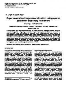
2. BAND-LIMITED EXTRAPOLATION We assume throughout this section that F共r兲 is defined for real r and is nonzero only for 兩r兩 艋 ⍀, where 0 ⬍ ⍀ ⬍ ␲. In addition, we assume that our data are f共m兲 , m = −M , … , M, that is, we have (possibly noisy) measurements of its Fourier transform f共x兲. Because ⍀ ⬍ ␲, the data are over-sampled; the Nyquist rate is ⌬ = ␲ / ⍀ ⬎ 1. The minimum-norm estimate FDFT in Eq. (8) does not involve the value ⍀ and estimates F共r兲 over the interval 关−␲ , ␲兴 associated with the actual sampling rate of unity. As simulations readily illustrated in Fig. 1, this DFT esti-

mate can do a poor job of recovering the finer detail of F共r兲 within its true support 关−⍀ , ⍀兴 because it wastes its limited degrees of freedom describing the values F共r兲 = 0 that occur for r outside 关−⍀ , ⍀兴. In addition, if we simply restrict the DFT to variables r within 关−⍀ , ⍀兴 and set our estimate of F共r兲 to zero outside, we have an estimate that is no longer consistent with the data. The goal of bandlimited extrapolation is to find a function that is both consistent with the measured Fourier-transform data and supported on the interval 关−⍀ , ⍀兴. Because F共r兲 is zero outside the interval 关−␲ , ␲兴 it has a Fourier-series representation within 关−␲ , ␲兴: ⬁

F共r兲 =

兺

The Gerchberg–Papoulis (GP) band-limited extrapolation method1,2 is an iterative procedure for estimating those F共m兲 for 兩m兩 ⬎ M. The procedure begins with zeros in place of all the f共m兲 for 兩m兩 ⬎ M and the data for the others. By use of those Fourier coefficients the resulting Fourier series is the DFT. The DFT is then truncated outside 关 −⍀ , ⍀兴 and the Fourier coefficients of this new function are computed. These new coefficients no longer match the measured data for 兩m兩 艋 M and so are replaced by the measured data; the other coefficients are left unchanged and the new Fourier series is formed. The resulting function of r is no longer zero outside 关−⍀ , ⍀兴 and so is truncated, as before. Repeating this, we obtain an iterative algorithm that converges to a function H共r兲 that is both consistent with the measured data and supported on the interval 关−⍀ , ⍀兴. Its Fourier series has coefficients that extrapolate the measured data, hence the name of the procedure. The GP algorithm as just described is not a practical method; it requires that we calculate an infinite set of Fourier coefficients at each step. One way around this is to discretize the problem and represent F共r兲 as a finite vector. The iteration can then be performed using the fast Fourier transform; this is the actual GP algorithm as used in practice. There is a second way around the practical problem, however. As pointed out in Ref. 7 (see also Ref. 8, p. 209), the function H共r兲 to which the theoretical GP method converges has the form M

H共r兲 = ␹⍀共r兲

兺

an exp共inr兲,

共10兲

n=−M

where ␹⍀共r兲 = 1 for 兩r兩 艋 ⍀ and is zero otherwise, and the am are such as to make H共r兲 consistent with the measured data. This means that the an satisfy the equations

f共m兲 =

兺

n=−M

DFT estimation from noiseless data.

共9兲

f共m兲exp共imr兲.

m=−⬁

M

Fig. 1.

259

an

sin关⍀共m − n兲兴

␲共m − n兲

,

共11兲

for n = −M , … , M; note that the value of the function sin共x兲 / x is defined by continuity to be one at x = 0. The Fourier transform of FMDFT共r兲 is

260

J. Opt. Soc. Am. A / Vol. 23, No. 2 / February 2006

Shieh et al.

冕

⍀

M

兺

−⍀兩F共r兲 −

an exp共inr兲兩2dr.

n=−M

These iterative and noniterative methods are usually called superresolution techniques in the signal-processing literature. Similar methods applied in sonar and radar array processing are called superdirective methods.9 In Figs. 1–3 we see the improvement, both in resolution achieved by the MDFT, compared with the DFT, and in the accuracy of the extrapolated Fourier-transform values. The vertical dashed line in each spectrum figure indicates the boundary of the data support. In particular, the form of the estimator in Eq. (10) is suggestive and leads to a more general MWN estimation procedure, called the prior DFT (PDFT) method (see below). Fig. 2. MDFT estimate with ⍀ = 1.8 from noiseless data (a) in spatial domain, (b) in spectrum domain.

3. PRIOR DISCRETE FOURIER TRANSFORM Prior information about the support of the function F共r兲 is incorporated in the FMDFT共r兲 estimator in Eq. (10) through the multiplicative factor ␹⍀共r兲. If we have prior information about the shape of the function 兩F共r兲兩 we can incorporate this information in a function P共r兲 艌 0 and replace ␹⍀共r兲 with P共r兲 as the first factor in the estimator. Because the second factor has the algebraic form of the DFT we call this new estimator the PDFT.10,11 The PDFT estimate of F共r兲 is then M

FPDFT共r兲 = P共r兲

兺

bn exp共inr兲,

共13兲

n=−M

with the bn satisfying the equations M

f共m兲 =

兺

bnp共m − n兲,

共14兲

n=−M

for n = −M , … , M, and Fig. 3. MDFT estimate with ⍀ = 0.9 from noiseless data (a) in spatial domain, (b) in spectrum domain.

M

fMDFT共x兲 =

兺

n=−M

an

sin关⍀共x − n兲兴

␲共x − n兲

,

共12兲

We can use the Fourier transform of the MDFT estimate as a data-extrapolation procedure, whereby f共x兲 is estimated by fMDFT共x兲. The behavior of this reconstruction method depends heavily on properties of the matrix B with entries Bmn = sin关⍀共m − n兲兴 / 关␲共m − n兲兴, as we shall see. This noniterative implementation of the theoretical GP algorithm, called the modified DFT (MDFT) in Ref. 7, can be viewed as a MWN solution to the reconstruction problem. The H共r兲 = FMDFT共r兲 described by Eqs. (10) and (11) is the function consistent with the data that minimizes the energy over the interval 关−⍀ , ⍀兴, given by 兰⍀−⍀兩H共r兲兩2dr. It is also the optimal approximation of F共r兲 of its form, in the sense that the coefficients an obtained using Eq. (11) minimize

1 p共x兲 =

2␲

冕

␲

P共r兲exp共− ixr兲dr.

共15兲

−␲

Note that, if P共r兲 = ␹⍀共r兲, then p共x兲 = sin共⍀x兲 / 共␲x兲. As in the case of the MDFT, the PDFT can be viewed as a data-extrapolation procedure. With the coefficients bn determined by Eq. (14), the Fourier transform of FPDFT共r兲 is M

fPDFT共x兲 =

兺

bnp共x − n兲.

共16兲

n=−M

The data extrapolation is achieved here through the use of a model of f共x兲 as a sum of translations of a positivedefinite kernel function. In a recent paper12 Poggio and Smale discuss the use of positive-definite kernels for interpolation, in the context of artificial intelligence and supervised learning. The weighted energy of FPDFT共r兲, given by 兰兩FPDFT共r兲兩2P共r兲−1dr, is the smallest among all functions defined on the support of P共r兲 and consistent with the data; therefore, the PDFT estimate is a MWN estimate. In addition, the coefficients bn found using Eq. (14) minimize

Shieh et al.

Vol. 23, No. 2 / February 2006 / J. Opt. Soc. Am. A

261

similar sense our finite data also tell us nothing about the value of ⍀; we can select any interval 关a , b兴 and find a function H共r兲 supported on 关a , b兴 whose h共x兲 is consistent with the data. But this is not quite the whole story; finite data cannot rule out anything, but they can suggest strongly that certain things are false. For example, let us select an interval 关a , b兴 disjoint from 关−⍀ , ⍀兴, and find the function H共r兲 consistent with the data, that is, with f共m兲 =

冕

b

a

Fig. 4. MDFT estimate with ⍀ = 0.9 from noiseless data (the true support is between −7␲ / 8 and −3␲ / 8 (a) in spatial domain, (b) in spectrum domain.

冕

␲

M

兩F共r兲 − P共r兲

−␲

兺

bn exp共inr兲兩2P共r兲−1dr,

dr H共r兲exp共− imr兲

2␲

,

for m = −M , … , M, for which the energy over 关a , b兴 , 兰ab兩H共r兲兩2dr, is minimum. Then this function H共r兲 will probably have large energy compared with that of the MDFT; that is, the integral 兰ab兩H共r兲兩2dr will be much ⍀ 兩FMDFT共r兲兩2dr, as clearly shown in Fig. 4. larger than 兰−⍀ We can use this fact to help us decide if we have chosen a good value for ⍀. In Ref. 16 this same idea was used to obtain an iterative algorithm for solving the phaseretrieval problem.

共17兲

n=−M

so the PDFT estimate is the function of its form closest to F共r兲, in the weighted-distance sense. Once again, the behavior of the estimation procedure will depend heavily on the properties of the matrix P whose entries are Pmn = p共m − n兲. Although we have discussed the MDFT and PDFT within the context of reconstructing F共r兲 from Fouriertransform values, both procedures extend in an obvious manner to any linear-functional data and to multivariate r. Of particular interest is the reconstruction of nonnegative functions F共r兲 from finitely many Fourier-transform values. The PDFT cannot include a nonnegativity constraint. However, the PDFT can be viewed as a linearized approximation of the minimum cross-entropy solution, which does impose nonnegativity. If we minimize the cross-entropy

冕

4. SENSITIVITY TO NOISE AND MODEL ERROR To use the MDFT we need the data to be oversampled and we need a decent estimate of the true support of the function F共r兲. The more oversampled the data and the more accurately we know the true support, the greater the improvement in resolution, but also the greater the sensitivity to noise and model error. Our goal in this section is to see why this is the case. The matrix B used in the MDFT has the entries Bmn = sin关⍀共m − n兲兴 / 关␲共m − n兲兴, with Bmm = ⍀ / ␲. Loosely speaking, B has 共⍀ / ␲兲共2M + 1兲 eigenvalues near one and the remaining eigenvalues near zero, as shown in Fig. 5. Solving Eqs. (11) is therefore an ill-conditioned problem, as ⍀ grows smaller. For the remainder of this section we denote by ␭1 ⬎ ␭2 ⬎ ¯ ⬎ ␭2M+1 ⬎ 0 the eigenvalues of B, with n , … , unM兲T, associated orthonormal eigenvectors un = 共u−M for n = 1 , … , 2M + 1. The matrix B then has the form

H共r兲 H共r兲log

P共r兲

+ P共r兲 − H共r兲dr

over all nonnegative H共r兲 consistent with the Fouriertransform data, the solution is

冋兺 M

FMCE共r兲 = P共r兲exp

n=−M

册

cn exp共inr兲 ,

with the cn chosen for consistency with the data.13–15 When we replace the exponential factor with a first-order linear approximation we get the PDFT. The goal of estimating F共r兲 from finite linear-functional data is somewhat paradoxical. The finite data we have tell us nothing, by themselves, about the values f共n兲 we have not measured. Using the MDFT, we can define f共M + 1兲 any way we wish and still construct an FMDFT共r兲 supported on the interval 关−⍀ , ⍀兴, and consistent with the original data and with this chosen value of f共M + 1兲. In a

Fig. 5. Eigenvalues of the matrix B (a) corresponding to ⍀ = 1.8, (b) corresponding to ⍀ = 0.9.

262

J. Opt. Soc. Am. A / Vol. 23, No. 2 / February 2006

Shieh et al.

2M+1

兺

B=

␭nun共un兲† ,

共18兲

n=1

so that 2M+1

B

−1

兺

=

␭n−1un共un兲† .

共19兲

n=1

We also denote by Un共r兲 the functions M

兺

Un共r兲 =

n um exp共imr兲.

m=−M

Since the eigenvectors are orthonormal we have

冕

␲

Uk共r兲Un共r兲dr = 0,

−␲

for k ⫽ n and

冕

␲

Un共r兲Un共r兲dr =

−␲

冕

␲

兩Un共r兲兩2dr = 1.

−␲

Also

冕

⍀

兩Un共r兲兩2dr = 共un兲†Qun = ␭n .

−⍀

Therefore, ␭n is the proportion of the energy of Un共r兲 for r in the interval 关−⍀ , ⍀兴. The function U1共r兲 is the most concentrated in that interval, while U2M+1共r兲 is the least. In Fig. 6 the typical behaviors of Un共r兲 for an example with 15 data are demonstrated. The function U1共r兲 has a single large main lobe and no zeros within 关−⍀ , ⍀兴. The function U2共r兲, being orthogonal to U1共r兲, but still largely concentrated within 关−⍀ , ⍀兴, has a single zero in that interval. Each succeeding function has one more zero within 关−⍀ , ⍀兴 and is somewhat less concentrated there than its predecessors. At the other extreme, the function U2M+1共r兲 has 2M zeros in 关−⍀ , ⍀兴, is near zero throughout that interval, and is concentrated mainly outside the interval. Because the eigenvectors are orthonormal the DFT estimate in Eq. (8) can be written in terms of these Un共r兲: 2M+1

FDFT共r兲 =

兺

n=1

关共un兲†d兴Un共r兲.

共20兲

Similarly, using Eq. (19), the MDFT estimate in Eq. (10) can be written as 2M+1

FMDFT共r兲 =

兺

n=1

␭n−1关共un兲†d兴Un共r兲.

共21兲

Comparing Eqs. (20) and (21) we see that the MDFT places greater emphasis on those Un共r兲 corresponding to larger values of n. These are the functions least concentrated within the interval 关−⍀ , ⍀兴, but they are also those with the greatest number of zeros within that interval. That means that these functions are much more oscillatory within 关−⍀ , ⍀兴 and better suited to resolve closely spaced peaks in F共r兲. Because the inner product 共un兲†d can be written as

Fig. 6. Example showing the absolute values of Un共r兲 for n = 1, 2,…,15, where their corresponding eigenvalues are (a) 1.00, (b) 9.99⫻ 10−1, (c) 9.82⫻ 10−1, (d) 8.29⫻ 10−1, (e) 4.02⫻ 10−1, (f) 7.82 ⫻ 10−2, (g) 6.83⫻ 10−3, (h) 3.52⫻ 10−4, (i) 1.21⫻ 10−5, (j) 2.91 ⫻ 10−7, (k) 4.85⫻ 10−9, (l) 5.53⫻ 10−11, (m) 4.12⫻ 10−13, (n) 1.72 ⫻ 10−15, (o) 4.28⫻ 10−18. Two vertical dashed lines indicate the boundaries of the prior support.

共un兲†d =

1 2␲

冕

␲

F共r兲Un共r兲dr,

−␲

this term will be relatively small for the larger values of n n † and so the product ␭−1 n 关共u 兲 d兴 will not be excessively large, provided that we have selected ⍀ properly. If ⍀ is too small and the support of F共r兲 extends beyond the interval 关⍀ , ⍀兴, then the term 共un兲†d will not be as small n † and the product ␭−1 n 关共u 兲 d兴 will be too large. This is what happens when there is noise in the data; the object function corresponding to the noisy data is not simply F共r兲 but contains a component that can be viewed as extending throughout the interval 关−␲ , ␲兴, as shown in Fig. 7. To reduce the sensitivity to noise while not sacrificing resolution, we regularize. The simplest way to do this is to add a small positive quantity, ⑀ ⬎ 0, to each of the diagonal elements of the matrix B. This is equivalent to modifying the MDFT to a PDFT in which the prior P共r兲 consists of two components, one the original ␹⍀共r兲, the second a small positive multiple of ␹␲共r兲. The effect of this regularization is to increase each of the ␭n by ⑀ without altering the eigenvectors or the Un共r兲. Since we now have 1 / 共␭n + ⑀兲 instead of the (potentially) much larger 1 / ␭n in Eq. (21), the sensitivity to noise and to poor selection of the ⍀ is reduced, as shown in Fig. 8. At the same time, however, we have reduced the importance for the MDFT of the Un共r兲 for larger values of n; this will lead to a loss of resolution and an MDFT that behaves like the DFT if ⑀ is too large, as shown in Fig. 9. Selecting the proper ⑀ is a bit of an art;

Shieh et al.

Vol. 23, No. 2 / February 2006 / J. Opt. Soc. Am. A

263

it will certainly depend on what the eigenvalues are and on the signal-to-noise ratio. The eigenvalues, in turn, will depend on the ratio ⍀ / ␲. We have focused here on a particular case in which the variable r is one-dimensional and the prior P共r兲 = ␹⍀共r兲 describes only the support of the object function F共r兲. For other choices of P共r兲, the eigenvalues of the corresponding matrix P are similarly behaved and ill conditioning is still an important issue, although the distribution of the eigenvalues may be somewhat different. For twodimensional r the support of F共r兲 can be described using a prior P共r兲 that is nonzero on a rectangle, on a circle, on an ellipse, or on a more general region. For each of those choices, the corresponding matrix will have eigenvalues that decay toward zero, but perhaps at different rates.

5. PHASE PROBLEM In optical image processing and elsewhere we find that we are unable to measure the complex values of the Fourier

Fig. 7. PDFT estimate with ⍀ = 0.7 (smaller than the true support) from noiseless data (a) in spatial domain, (b) in spectrum domain.

Fig. 9. PDFT estimate with ⍀ = 0.9 from noisy data 共⑀ = 0.1兲 (a) in spatial domain, (b) in spectrum domain.

transform f共xm兲, only the magnitudes 兩f共xm兲兩. Estimating F共r兲 from these magnitude-only values is called the phase problem.17–21 Such problems can arise in optical imaging through turbulent atmosphere.22 One solution to the phase problem in crystallography led to a Nobel Prize in 1985 for Jerome Karle. Assume now that F共r兲 = 0 for 兩r兩 ⬎ ⍀. We can select an arbitrary collection of phases ␪m to combine with the magnitudes, to form the complex pseudodata 兩f共xm兲兩ei␪m. If we have some idea of the proper choice of ⍀, we calculate the estimate FMDFT共r兲 corresponding to the pseudodata and again monitor the energy integral. For good choices of the phases, the energy should not be too large, while, for inappropriate choices, the energy should be much larger, particularly if the data are oversampled. The reconstruction process can be implemented as an iterative optimization procedure, in which we select a new collection of phases at each step in such a way as to reduce the energy in the band-limited extrapolation that results. In Ref. 16 we show how to do this in an efficient manner. When the extrapolation energy is sufficiently small, the resulting estimate is typically acceptable, particularly when the data are oversampled. When we have only magnitude measurements, we can at least be sure that if 兩f共xm兲兩 = 0 then f共xm兲 = 0. This suggests that we might try to estimate the function F共r兲 from the zeros of its Fourier transform. In Ref. 23 we showed that this approach has some promise for solving the phase problem.

6. CALCULATING THE PRIOR DISCRETE FOURIER TRANSFORM

Fig. 8. PDFT estimate with ⍀ = 0.9 from noisy data 共⑀ = 0.001兲 (a) in spatial domain, (b) in spectrum domain.

When the data set is large, as usually happens in multidimensional problems such as image reconstruction, solving Eqs. (11) and (14) is sometimes done iteratively. Nevertheless, these algorithms still differ from the GP method based on a discretized model in that we are still extrapolating infinitely many values of f共n兲 and obtaining a continuous-function estimate; we are just doing it using a finite parameter model.

264

J. Opt. Soc. Am. A / Vol. 23, No. 2 / February 2006

Constructing the matrix P used in Eq. (14) can be difficult when the data sets are large. In such cases we can employ an iterative discrete implementation of the PDFT, the DPDFT, which allows us to avoid having to form this large matrix.24 The DPDFT reconstructs a finite-vector approximation of the function F共r兲. The linear-functional data are represented as inner products of this vector with finitely many known vectors. The number of data points we have is smaller than the dimension of the discretized object, so the reconstruction problem, which is now a system of linear equations to be solved, is still underdetermined. We use a discretized version of the reciprocal of the prior function P共r兲 to determine the weights and then calculate a MWN solution to the underdetermined system of equations. This is done using the algebraic reconstruction technique.13

Shieh et al.

relation function rs共k兲 = E共sn+ksn兲 and power spectrum Rs共␻兲 defined for ␻ in the interval 关−␲ , ␲兴, and 兵qn其 is the noise component with autocorrelation function rq共k兲 and power spectrum Rq共␻兲 defined for ␻ in 关−␲ , ␲兴. We assume that for each n the random variables sn and qn have mean zero and that the signal and noise are independent of one another. Then the autocorrelation function for the signalplus-noise sequence 兵zn其 is rz共n兲 = rs共n兲 + rq共n兲 for all n, and R z共 ␻ 兲 = R s共 ␻ 兲 + R q共 ␻ 兲 is the signal-plus-noise power spectrum. ⬁ Let h = 兵hk其k=−⬁ be a linear filter with transfer function ⬁

7. PRIOR DISCRETE FOURIER TRANSFORM AND OPTIMAL LINEAR DETECTION The problem of detecting a signal in additive noise uses the following model. The data vector z = 共z1 , … , zN兲T is assumed to be the sum z = ␥s + q

b=

e共␻兲†Q−1e共␻兲

Q−1e共␻兲,

and the optimal estimate of ␥ is

␥ˆ = b†z =

1 e共␻兲 Q−1e共␻兲 †

兺he k

ik␻

,

k=−⬁

for ␻ in 关−␲ , ␲兴. Given the sequence 兵zn其 as input to this filter, the output is the sequence ⬁

yn =

兺hz

k n−k .

共22兲

k=−⬁

of a signal component ␥s, where s = 共s1 , … , sN兲T and ␥ ⬎ 0, and a noise component q = 共q1 , … , qN兲T with mean E共q兲 = 0 and covariance matrix E共qq†兲 = Q.25 The estimation problem is to estimate ␥, given s and Q. The detection problem is to decide if ␥ is zero or not. In certain applications s is not known exactly, but is assumed to be a member of a parametrized family. For example, in the problem of detecting a sinusoidal component at an unknown frequency ␻ we take e共␻兲 to be the column vector with entries e共␻兲m = exp共imw兲. For fixed ␻ the optimal linear filter for estimating ␥ is 1

H共␻兲 =

e共␻兲†Q−1z.

The factor 1 / e共␻兲†Q−1e共␻兲 can be viewed as an estimate of the power spectrum associated with the covariances in Q,25 while the factor e共␻兲†Q−1z has the form of a DFT. Comparing this estimate of ␥ with the PDFT estimate of F共r兲 we see that the first factor, 1 / e共␻兲†Q−1e共␻兲, is playing a role analogous to that played by P共r兲, the matrix Q is analogous to the matrix P, and the factor e共␻兲†Q−1z corresponds to the sum that appears as the second factor in the PDFT. Although the matrix Q need not be Toeplitz, as P always is, the correspondence is interesting.

The goal of Wiener filtering is to select the filter h so that the output sequence 兵yn其 approximates the signal sequence 兵sn其 as well as possible. Specifically, we seek h so as to minimize the expected squared error, E共兩yn − sn兩2兲, which, because of stationarity, is independent of n. Minimizing E共兩yn − sn兩2兲 with respect to the function H共␻兲 leads to the equation Rz共␻兲H共␻兲 = Rs共␻兲, so that the transfer function of the optimal filter is H共␻兲 = Rs共␻兲/Rz共␻兲. The Wiener filter is then the sequence 兵hk其 of the Fourier coefficients of this function H共␻兲. Since H共␻兲 is a nonnegative function of ␻, therefore real-valued, its Fourier coefficients hk will be conjugate symmetric; that is, h−k = hk. Therefore, the Wiener filter is not causal; this poses a problem when the random process zn is a discrete time series, with zn denoting the measurement recorded at time n. To remedy this we can obtain the best causal approximation of the Wiener filter h. Even having a causal filter does not completely solve the problem, since we would have to record and store the infinite past. Instead, we can decide to use a filter f ⬁ for which fk = 0 unless −K 艋 k 艋 L for some posi= 兵fk其k=−⬁ tive integers K and L. This means we must store L values and wait until time n + K to obtain the output for time n. Such a linear filter is a finite-memory–finite-delay filter, also called a finite-impulse-response (FIR) filter. Given the input sequence 兵zn其 the output of the FIR filter is L

8. PRIOR DISCRETE FOURIER TRANSFORM AND WIENER FILTER APPROXIMATION Suppose now that the discrete stationary random process to be filtered is the doubly infinite sequence 兵zn = sn ⬁ + qn其n=−⬁ , where 兵sn其 is the signal component with autocor-

vn =

兺fz

k n−k .

k=−K

To obtain such an FIR filter f that best approximates the Wiener filter, we find the coefficients fk that minimize the quantity E共兩yn − vn兩2兲, or, equivalently,

Shieh et al.

Vol. 23, No. 2 / February 2006 / J. Opt. Soc. Am. A

冕

␲

L

兩H共␻兲 −

−␲

兺fe k

ik␻ 2

兩 Rz共␻兲d␻ .

共23兲

k=−K

The orthogonality principle tells us that the optimal coefficients must satisfy the equations

265

Fourier-transform data; is closely related to Wiener-filter approximation, which suggests a nonlinear reconstruction procedure leading to entropy-maximization techniques; and provides a unifying model for resolution enhancement and data extrapolation. Hsin M. Shieh’s e-mail address is [email protected].

L

rs共m兲 =

兺 f r 共m − k兲, k z

for − K 艋 m 艋 L.

共24兲

k=−K

In Ref. 26 it was pointed out that the minimization in relation (23) is analogous to that in relation (17), with Rz共␻兲 and Rs共␻兲 playing the roles of P共r兲 and F共r兲, respectively. In the PDFT we do not require that F共r兲 be nonnegative-valued, however. If we switch the roles, viewing Rz共␻兲 and Rs共␻兲 as F共r兲 and P共r兲, respectively, we obtain nonlinear reconstruction methods containing, as a particular case, the Burg entropy-maximization estimator for the case of nonnegative F共r兲.27

9. CONCLUSIONS In summary, an important concern in image reconstruction is the validity and reliability of the resulting image. When one has only limited, sampled noisy data, it makes no sense to consider image restoration or superresolution in the absence of a model that incorporates prior knowledge of the scene or target being imaged. The incorporation of prior knowledge has deep implications because it impacts how one might interpret the information capacity of an optical imaging system while fixing the numbers of degrees of freedom that the system possesses. Image reconstruction techniques also demand measures of image quality; these are very difficult to agree upon and yet are needed and important. By offering a more complete view of the methods for image restoration and data extrapolation here, and in showing the relationships that exist between such methods, we are laying a foundation to address the fundamental problem of assessing the information content of data and of the resulting processed image. We have shown that improved resolution in reconstructing an image from limited, noisy data can be achieved through the use of minimum-weighted-norm (MWN) data extrapolation. The weighted norm is chosen to incorporate prior knowledge of object support or overall shape. The resulting object-function estimate is a dataconsistent model that can be viewed as extrapolating the data, thereby improving resolution. To understand precisely how improved resolution is achieved, why the reconstruction can be sensitive to noise in the data, and how this sensitivity is reduced, we have examined the eigenvectors and eigenvalues of the Gramian matrix describing the data-collection process. We found that the eigenvectors associated with the smallest eigenvalues are responsible both for the improved resolution and the greater sensitivity. Regularization enables us to maintain higher resolution while reducing sensitivity. The improvement in reconstruction is observed in object space, where the reconstruction is compared to the original object, as well as in data space, where we can judge success in extrapolating beyond the data window. The MWN paradigm for reconstruction includes band-limited extrapolation of

REFERENCES 1. 2. 3. 4. 5. 6.

7.

8. 9. 10. 11.

12. 13.

14. 15.

16. 17. 18. 19. 20.

R. W. Gerchberg, “Super-restoration through error energy reduction,” Opt. Acta 21, 709–720 (1974). A. Papoulis, “A new algorithm in spectral analysis and band-limited extrapolation,” IEEE Trans. Circuits Syst. 22, 735–742 (1975). J. Burg, “Maximum entropy spectral analysis,” presented at the 37th Annual Society of Exploration Geophysicists Meeting, Oklahoma City, Oklahoma, July 1967. J. Burg, “The relationship between maximum entropy spectra and maximum likelihood spectra,” Geophysics 37, 375–376 (1972). J. Burg, “Maximum Entropy Spectral Analysis,” Ph.D. thesis (Stanford University, Stanford, California, 1975). M. Bertero, “Sampling theory, resolution limits and inversion methods,” in Inverse Problems in Scattering and Imaging, M. Bertero and E. R. Pike, eds. (Malvern Physics Series, Adam Hilger, IOP Publishing, 1992), pp. 71–94. C. L. Byrne and R. M. Fitzgerald, “A unifying model for spectrum estimation,” presented at the Rome Air Development Center Workshop on Spectrum Estimation, Griffiss Air Force Base, Rome, New York, October 3–5, 1979. H. Stark and Y. Yang, Vector Space Projections: A Numerical Approach to Signal and Image Processing, Neural Nets and Optics (Wiley, 1998). H. Cox, “Resolving power and sensitivity to mismatch of optimum array processors,” J. Acoust. Soc. Am. 54, 771–785 (1973). C. L. Byrne and R. M. Fitzgerald, “Reconstruction from partial information, with applications to tomography,” SIAM J. Appl. Math. 42, 933–940 (1982). C. L. Byrne, R. M. Fitzgerald, M. A. Fiddy, T. J. Hall, and A. M. Darling, “Image restoration and resolution enhancement,” J. Opt. Soc. Am. 73, 1481–1487 (1983). T. Poggio and S. Smale, “The mathematics of learning: dealing with data,” Not. Am. Math. Soc. 50, 537–544 (2003). R. Gordon, R. Bender, and G. T. Herman, “Algebraic reconstruction techniques (ART) for three-dimensional electron microscopy and x-ray photography,” J. Theor. Biol. 29, 471–481 (1970). C. L. Byrne, “Iterative image reconstruction algorithms based on cross-entropy minimization,” IEEE Trans. Image Process. IP-2, 96–103 (1993). C. L. Byrne, “Erratum and addendum to ‘Iterative image reconstruction algorithms based on cross-entropy minimization’,” IEEE Trans. Image Process. IP-4, 225–226 (1995). C. L. Byrne and M. A. Fiddy, “Estimation of continuous object distributions from Fourier magnitude measurements,” J. Opt. Soc. Am. A 4, 412–417 (1987). M. A. Fiddy, “The phase retrieval problem,” in Inverse Optics, A. Devaney, ed., Proc. SPIE 413, 176–181 (1983). J. C. Dainty and M. A. Fiddy, “The essential role of prior knowledge in phase retrieval,” Opt. Acta 31, 325–330 (1984). J. Fienup, “Reconstruction of a complex-valued object from the modulus of its Fourier transform using a support constraint,” J. Opt. Soc. Am. A 4, 118–123 (1987). R. Lane, “Recovery of complex images from Fourier magnitude,” Opt. Commun. 63, 6–10 (1987).

266 21.

22. 23. 24.

J. Opt. Soc. Am. A / Vol. 23, No. 2 / February 2006 J. Cederquist, J. Fienup, C. Wackerman, S. Robinson, and D. Kryskowski, “Wave-front phase estimation from Fourier intensity measurements,” J. Opt. Soc. Am. A 6, 1020–1026 (1989). J. Fienup, “Space object imaging through the turbulent atmosphere,” Opt. Eng. (Bellingham) 18, 529–534 (1979). C.-W. Liao, M. A. Fiddy, and C. L. Byrne, “Imaging from the zero locations of far-field intensity data,” J. Opt. Soc. Am. A 14, 3155–3161 (1997). H. M. Shieh, M. E. Testorf, C. L. Byrne, and M. A. Fiddy,

Shieh et al.

25. 26. 27.

“Iterative image reconstruction using prior knowledge,” submitted to J. Opt. Soc. Am. A. C. L. Byrne, Signal Processing: A Mathematical Approach (AK Peters, 2005). C. L. Byrne and M. A. Fiddy, “Images as power spectra; reconstruction as Wiener filter approximation,” Inverse Probl. 4, 399–409 (1988). C. L. Byrne and R. M. Fitzgerald, “Spectral estimators that extend the maximum entropy and maximum likelihood methods,” SIAM J. Appl. Math. 44, 425–442 (1984).