Image representations for object detection using

Image representations for object detection using kernel classifiers Theodoros Evgeniou, Massimiliano Pontil,Constantine Papageorgiou, and Tomaso Poggio Center for Biological and Computational Learning, MIT 45 Carleton Street E25-201, Cambridge, MA 02142, USA e-mail: {theos,pontil,cpapa,tp}@ai.mit.edu Abstract This paper presents experimental comparisons of various image representations for object detection using kernel classifiers. In particular it discusses the use of support vector machines (SVM) for object detection using as image representations raw pixel values, projections onto principal components, and Haar wavelets. General linear transformations of the images through the choice of the kernel of the SVM are considered. Experiments showing the effects of histogram equalization, a non-linear transformation, are presented. Image representations derived from probabilistic models of the class of images considered, through the choice of the kernel of the SVM, are also evaluated. Finally, we present a feature selection method using SVMs, and show experimental results. Keywords: Support Vector Machines, Kernel, Wavelets, PCA, histogram equalization.

1. Introduction Detection of real-world objects in images, such as faces and people, is a challenging problem of fundamental importance in many areas of image processing: the objects are difficult to model, there is significant variety in color and texture, and the backgrounds against which the objects lie are unconstrained. We have chosen a learning based approach to object detection and focused on the use of Support Vector Machines (SVM) classifiers [20] as the core engine of these systems [15]. A major issue in such a system is choosing an appropriate image representation. This paper presents experimental results comparing different image representations for object detection, in particular for detecting faces and people. Initial work on object detection used template matching approaches with a set of rigid templates or handcrafted parameterized curves, Betke & Makris[1], Yuille, et al.[23]. These approaches are difficult to extend to more complex objects such as people, since they involve a significant amount of prior information and domain knowledge. In recent research the detection problem has been solved using learning-based techniques that are data driven. This approach was used by Sung and Poggio[17] and Vaillant, et al. [19] for the detection of frontal faces in cluttered scenes, with similar architectures later used by Moghaddam and Pentland [10], Rowley, et al.[16], and Osuna et al.[12]. A variety of image representations have been used in these works. In this paper we compare some of them that we also link through the choice of kernels in the SVM classifier, and discuss novel ones derived from probabilistic models.

2. Background We briefly describe the trainable system for object detection that we used in this work. The system is based on [15] and can be used to learn any class of objects. The overall framework has been motivated and successfully applied in the past [15]. The system consists of three parts: (i) a set of (positive) example images of the object class considered (i.e. images of frontal faces) and a set of negative examples (i.e. any non-face image) are collected. (ii) The images are transformed into vectors in a chosen representation (i.e. a vector of the size of the image with the values at each pixel location - below this is called the “pixel” representation). (iii) The vectors (examples) are used to train a SVM classifier to learn the classification task of separating positive from negative examples. A new set of examples is used to test the system. The full architecture involves scanning an (test) image over different positions and scales. We refer to [15] for more information. Two choices need to be made: the representation in the second stage, and the kernel of the SVM (see below) in the third stage. This paper focuses on these two choices. In the experiments described below, we used the following data: for the face detection systems, we used 2,429 positive images of frontal faces of size 19x19, and 13,229 negative images randomly chosen from large images not containing faces, like in [15]. The systems were tested on new data consisting of 105 positive images and around 4 million negative ones. For the people detection systems, we had 700 positive images of people of size 128x64, and 6,000 negative images, like in [11]. The systems were tested on new data consisting of 224 positive images and 3,000 negative ones (for computational reasons, only for Figure 3 we used more test points: 123 positive and around 800,000 negative ones). The performances are compared using ROC curves [15] generated by moving the hyperplane of the SVM solution by changing the threshold b (see below), and computing the percentage of false positives and false negatives for each choice of b. In the plots presented the vertical axis shows the percentage of positive test images correctly detected (1 - false negative percentage), while the horizontal axis shows one false positive detection per number of negative test images correctly classified.

2.1. Support Vector Machine classification Support vector machines (SVM) is a technique to train classifiers that is well-founded in statistical learning

αi yi K(x, xi ) + b

i=1

!

(1)

where ℓ is the number of training data points (xi , yi ) (yi being the label ±1 of training point xi ), αi are nonnegative parameters learned from the data, and K(·, ·) is a kernel that defines a dot product between projections of the two arguments in some feature space [20, 22] where a separating hyperplane is then found. For example, when K(x, y) = x · y is the chosen kernel, the separating surface is a hyperplane in the space of x (input space). The kernel K can be a Gaussian (Radial Basis Functions [6]), or an nth degree polynomial (x · y + 1)n , and generally any positive definite function [20, 22]. The main feature of SVM is that it finds, among all possible separating surfaces of the form (1), the one which maximizes the distance between the two classes of points (as measured in the feature space defined by K). The support vectors are the nearest points to the separating boundary and are the only ones (typically a small fraction of the training data) for which αi in equation (1) is positive. The distance of the closest one from the boundary is: 

d=

ℓ X

i,j=1

− 12

αi αj yi yj K(xi , xj )

(2)

The intra-class distance, also called margin, is twice the distance of a support vector from the boundary, 2d. The margin is an important quantity because it can be taken as an indicator of the separability of the data and consequently of the “goodness” of the representation 2 used. In fact the quantity R d2 , with R being the radius of the smallest sphere containing the data points, is the VC-dimension of the SVM [20]. It may be that different input representations and/or kernel functions lead to quite different geometries of the data (i.e. different margins), which in turn influences the performance of the SVM.

3. Comparison of representations for face and people detection 3.1. Pixels, principal components and Haar wavelets Using the experimental setup described above, we conducted experiments to compare the discriminative power of three different image representations: (i) The pixel representation: train an SVM using the raw pixel values scaled between 0 and 1 (i.e. for faces this means that the inputs to the SVM machine are 19 · 19 = 361 dimensional vectors with values from 0 to 1 - before scaling it was 0 to 255). (ii) The eigenvector (principal components) representation: compute the correla-

Pixels vs PCA vs Wavelets 1

Detection Rate

f (x) = θ

ℓ X

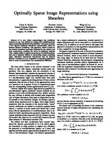
tion matrix of the positive examples (their pixel vectors) and find its eigenvectors. Then project the pixel vectors on the computed eigenvectors. We can either do a full rotation by taking the projections on all 361 eigenvectors, or use the projections on only the first few principal components. We discuss this issue in section 3. We rescaled the projections to be between 0 and 1. (iii) The wavelet representation: consider a set of Haar wavelets at different scales and locations, and compute the projections of the image on the chosen wavelets. For the face detection experiments we used all wavelets (horizontal, vertical and diagonal) at scales 4×4 and 2×2 since their dimensions correspond to typical features for the size of the face images considered. We had a total of 1,740 coefficients for each image. For the people detection system we considered wavelets at scales 32 × 32 and 16 × 16 shifted by 8 and 4 pixels respectively. We had a total of 1,326 coefficients. We rescaled the outputs of the projections to be between 0 and 1. Figure 1 shows the results of the experiments comparing the representations described above. In all these experiments a second order polynomial kernel was used. The motivation for using such a kernel is based on the experimental results of [13, 15]. Throughout the paper, notice the range of the axis in all the plots in the figures: the range varies in order to show clearer the important parts of the curves.

0.8 0.6 0.4 0.2 −6

−5

10

−4

10

−3

10

10

1

Detection Rate

theory; for details, see [20, 2, 3]. One of the main attractions of using SVMs is that they are capable of learning in sparse, high-dimensional spaces with very few training examples (i.e. 10,000 dimensional data in [9], or 283 dimensional data in [13] - see also section 4). The separating boundary is in general of the form:

0.9 0.8 0.7 0.6

−3

10

−2

10 False Positive Rate

−1

10

Fig. 1: ROC curves for face (top) and people (bottom) detection: solid lines are for the wavelet representation, dashed lines for pixel representation, and dotted line for eigenvector representation (all 361 eigenvectors). These experiments suggest a few remarks. First notice that both the pixel and eigenvector representations give almost identical results (small differences due to the way the ROC curves are produced are ignored). This is an observation that has a theoretical justification that we discuss in section 3.2. Second, notice that for faces the wavelet representation performs about the same as the other two, but in the case of people, the wavelet representation is significantly better than the other two. This is a finding that was expected [15, 11]: for people pixels may not be very informative (i.e. people

may have different color clothes), while wavelets capture intensity differences that discriminate people from other patterns [15]. On the other hand, for faces at the scale we used, pixel values seem to capture enough of the information that characterizes faces. Notice that all the three representations considered so far are linear transformations of the pixels representation. This takes us to the next topic.

3.2. Linear transformations and kernels As discussed in section 2.2, a key issue when using a SVM is the choice of the kernel K in equation (1). The kernel K(xi , xj ) defines a dot product between the projections of two inputs xi , xj , in a feature space. Therefore the choice of the kernel is very much related to the choice of the “effective” representations of the images. In particular there is a simple relation between linear transformations of the original images, such as the ones considered above, and kernels. A point (image) x is linearly decomposed in a set of features c = c1 , . . . , cm by c = Ax, with A a real matrix (we can think of the features c as the result of applying a set of linear filters to the image x). If the kernel used is a polynomial of degree m∗ (as in the m experiments), then K(xi , xj ) = (1 + x⊤ i · xj ) , while ⊤ m ⊤ ⊤ K(ci , cj ) = (1+ci ·cj ) = (1+xi (A A)xj )m . So using a polynomial kernel in the “c” representation is ⊤ m the same as using a kernel (1 + x⊤ i (A A)xj ) in the original one. This implies that one can consider any linear transformation of the original images by choosing the appropriate square matrix AT A in the kernel K of the SVM. As a consequence of this observation, we have a theoretical justification of why the pixel and eigenvector representations lead to the same performance: in this case the matrix A is orthonormal, therefore AT A = I which implies that the SVM finds the same solution in both cases. On the other hand, if we choose only some of the principal components (like in the case of eigenfaces [18]), or if we project the images onto Haar wavelets, the matrix A is no longer orthonormal, so the performance of the SVM may be different.

3.3. Histogram Equalization We now discuss the experimental finding that histogram equalization (H.E.), a non-linear transformation of the “pixel” representation, improves the performance of the detection system on our databases of images. Given an image, H.E. is performed in two steps: first the pixel values (numbering 0 to 255) are grouped into a smallest number of bins so that the distribution of the number of pixels in the image is uniform among the bins; then we replace the pixel values of the original image with the values (rank) of the bins they fall into. More information on H.E. can be found in the literature (i.e. [8]). We tested the systems described in section 3.1, this ∗ Generally this holds for any kernel for which only dot products between input arguments are needed - i.e. also for Radial Basis Functions.

time after performing H.E. on every input image. Only for the wavelet representation, instead of projecting histogram equalized images on the chosen wavelets, we transformed the outputs of the projections of the original images on the wavelets using a sigmoid function. This operation is (almost) equivalent to first performing H.E. and then projecting on the wavelet filters the histogram equalized image (assuming Gaussianlike histogram of the original image). Figure 2 shows the performance of the detection system. Both for face and people detection the performance increased dramatically. H.E. has been extensively used for image compression and in this case it is straightforward to show that H.E. is a form of Vector Quantization [4] and is an effective coding scheme. Classification is however different from compression and it is an open question of why H.E. seems to improve so much the performance of our SVM classifier. Here we offer a conjecture: Suppose that a transformation satisfies the following two conditions: (a) it is a legal transformation of the input vector, that is it preserves the class label; (b) it increases the entropy of the input set, leading to a more compressed representation. We conjecture that such a transformation will improve the performance of a SVM classifier. Notice that H.E. is a transformation of the images that satisfies the above conditions: i.e. faces remain faces, and non-faces remain non-faces (of course one can design images where this does not hold, but such images are very unlikely and are not expected to exist among the ones we used for training and/or testing). Moreover H.E. leads to a more compressed representation of the images (in terms of bits needed to describe them). Of course the first condition relies on prior information. In the case of H.E. applied to images we know a priori that H.E. is a transformation embedding “illumination invariance”: images of the same face under different illuminations can be mapped into the same vector under H.E. Thus performing an H.E. transformation is roughly equivalent to using a larger training set containing many “virtual examples” generated from the real examples [5, 21] by changing the global illumination (mainly the dynamic range). Of course a larger training set in general improves the performance of a classifier. So this may explain the improvement of the system. In general, because of the same arguments outlined above, we expect that any transformation of the original images that “effectively” takes advantage of prior information about the class of images considered and compresses their signatures, is expected to improve the performance of the system.

4. Input feature selection using SVM This section addresses the following questions: can feature selection improve performance of the SVM classifier? can SVM perform well even when many (possibly irrelevant) features are used? In order to investigate these issues, we performed several experiments where the object detection systems were trained with different numbers of input features. To this pur-

Histogram Equalization

Detection Rate

1 0.8 0.6 0.4 0.2 −6

−5

10

−4

10

−3

10

10

component of vector xi . Notice that this is only an approximation to the actual derivative: changing the value of a feature may also lead to different solution of the SVM, namely different α’s. We assume that this change is small and we neglect it. To summarize, our feature selection method consists of computing the quantity in (3) for all the input features and selecting the ones with the largest values I r .

0.95

Feature Selection 1

0.9 0.5

0.85 0.8

−3

10

−2

10 False Positive Rate

0

−1

10

Fig. 2: ROC curves for face (top) and people (bottom) detection after histogram equalization: solid lines are for the wavelet, dashed lines for the pixel, and dotted line for the eigenvector representation. We also show the ROC curve for the wavelet representation without histogram equalization (like in Figure 1); this is the bottom thick solid line. For people, the bottom thick dashed line shows the performance of pixels without H.E.. pose we have developed a method for automatically selecting a Subset of the input features within the framework of SVM. The idea of the proposed feature selection method is based on the intuition that the most important input features are the ones for which, if removed or modified, the separating boundary f (x) = 0 changes the most. Instead of the change of the boundary we can consider the average change of the value of the function f (x) in a region around the boundary (variations of f will affect classification only for points near the boundary). To do so, we compute the derivative of f (x) with respect to an input feature xr and integrate the absolute value (we are interested in the magnitude of the derivative) in a volume V around the boundary: Z df r dP (x) r . I = dx V

In practice we cannot compute this quantity because we do not know the probability distribution P (x). Instead we can approximate Ir with the sum over the support vectors†: Nsv Nsv Nsv X X X r df = Ir ≈ α y K (x , x ) j j j i . (3) dxr i i=1 i=1 j=1

where Nsv is the number of support vectors and K r (xj , xi ) is the derivative of the kernel with respect to the rth dimension evaluated at xi . For example for K(xj , xi ) = (1 + xj · xi )2 , this is equal to K r (xj , xi ) = (1 + xj · xi )xri where xri is the rth † For separable data these are also the points nearest to the separating surface. For non-separable data we can take the sum over only the support vectors near the boundary.

−5

−4

10 Detection Rate

Detection Rate

1

−3

10

10

1 0.5 0 −6 10 1

−5

10

−4

10

−3

10

0.9 0.8 0.7 −4

−3

10

10 False Positive Rate

Fig. 3: Top figure: solid line is face detection with all 1,740 wavelets, dashed line is with 30 wavelets chosen using the proposed method, and dotted line is with 30 randomly chosen wavelets. The line with ×’s is with 500 wavelets, and the line with ◦’s is with 120 wavelets, both chosen using the method based on equation (3). Middle figure: solid line is face detection with all eigenvectors, dashed line is with the 40 principal components, and dotted line is with the 15 principal components. Bottom figure: solid line is people detection using all 1,326 wavelets, dashed line is with the 29 wavelets chosen by the method based on equation (3), and dotted line is with the 29 wavelets chosen in [15]. For people detection, using the proposed heuristic we selected 29 of the initial set of 1,326 wavelet coefficients. We then trained an SVM using only the 29 selected features and compared the performance of the machine with that of an SVM trained on 29 coefficients selected using a manual method as described in [15]. We show the results in Figure 3 (bottom plot). We also tested the same heuristic for face detection. We selected 30 of the initial 1,740 wavelet coefficients, and we compared the performance of an SVM trained using only these 30 features, with the performance of a SVM that uses 30 randomly selected features out of the initial 1,740. We also show the performance of the system when 500 of the wavelets were chosen. Notice that using the proposed method we can select about a third (500) of the original input dimensions without significantly decreasing the performance of the system. The result is also shown in Figure 3 (top plot). Finally for the eigenvector representation, we also tested the system using few principal components. The re-

5. Features from probabilistic models In this section we take a different approach to the problem of finding image representations. Consider a specific class of images (i.e. faces, people, cars) and assume that they are sampled according to a generative probabilistic model P (x|β), where β indicates a set of parameters. As an example consider a Gaussian distribution with P (x|β) being:   1 1 ⊤ −1 (4) exp − (x − x0 ) Σ (x − x0 ) d 1 2 2π 2 |Σ| 2 where the parameters β are the average image x0 and the covariance Σ. Recent work [14] shows how the assumption of a specific probabilistic model of the form (4) suggests a choice of the kernel – and therefore of the “features” – to be used in order to reconstruct, through the SVM regression algorithm, images of faces and people. The relevant features are the principal components un of the set of examples (i.e. faces or people) scaled by the corresponding eigenvalues λn . However, [14] left open the question of what features to choose in order to do classification as opposed to regression, that to discriminate faces (or people) from non-faces (nonpeople), once the probabilistic model is decided. Very recently a general approach to the problem of constructing features for classification starting from probabilistic models describing the training examples has been suggested [7]. The choice of the features was made implicitly through the choice of the kernel to be used for a kernel classifier. In [7] a probabilistic model for both the classes to be discriminated was assumed, and the results were also used when a model of only one class was available - which is the case we have. Let us denote with L(x|β) the log of the probability function and define the Fisher information matrix Z I = dxP (x|β)∂i L(x|β)∂j L(x|β), where ∂i indicates the derivative with respect to the parameter βi . A natural set of features, φi , is found by taking the gradient of L with respect to the set of parameters, 1

φi (x) = I − 2

∂L(x|β)) . ∂β

(5)

These features were theoretical motivated in [7] and shown to lead to kernel classifiers which are at least

as discriminative as the Bayes classifier based on the given generative model. We have assumed the generative model (4) and rewritten it with respect to the average image x0 and the eigenvalues λn and obtained the set of features according to equation (5). For simplicity the principal components were kept fixed in the model. The features obtained in this way were then used as a new input representation in our learning system. The resulting linear kernel K(xi , xj ) obtained by taking the dot product between the features (dot product for the implicitly chosen representation) of a pair of images xi and xj is: N X

2 2 [−λ−1 n (cn (xi ) − cn (xj )) + λn cn (xi )cn (xj )],

n=1

(6) where cn (x) = (x − x0 )⊤ un and N is the total number of eigenvectors (principal components) used. The parameters x0 , un , λn were estimated using the training examples of faces (or people). Note that we used the training data multiple times: once for estimating the probabilistic model (4), and once to train an SVM classifier. Equation (6) indicates that only a limited number of principal components can be used in practice because small λn create numerical instabilities in the learning algorithm. We performed several experiments by changing the number of principal components used in the model (see Figure 4) and compared the results with the image representations discussed in section 3. We notice that the proposed representation performs slightly better than the other ones (when 100 principal components were used), but not significantly better. It may be the case that features from other (more realistic) probabilistic models lead to better systems. Probabilistic Features 1

0.9

0.8 Detection Rate

sults are also shown in Figure 3 (middle plot). From all the experiments shown in Figure 3 we observe that SVMs are not sensitive to large numbers of input dimensions. In fact in all cases, when using all input dimensions (all wavelets or all eigenvectors) the system performed better (or about the same) than when using few of the input features. Our experimental finding gives a first answer, although not general and theoretical, to the questions asked at the beginning of this section: it confirms the difficulty of the feature selection problem, and indicates that SVMs work well even when the input data are high-dimensional, by automatically dealing with irrelevant features.

0.7

0.6

0.5

0.4 −6 10

−5

10

−4

10 False Positive Rate

−3

10

−2

10

Fig. 4: Face experiments: Solid line indicates the probabilistic features using 100 principal components, dashed line is for 30 principal components, and dotted for 15. We also show the ROC curves with all wavelets (line with circles) for comparison. Histogram equalization was performed on the images.

6. Conclusions and future work We have presented experiments for face and people detection with different image representations and kernels using SVM. We summarize the main points: (i) For face detection, pixels, principal components, and Haar wavelets perform almost equally well. (ii) For people detection, the Haar wavelet representation significantly outperforms the other two. (iii) We can capture all linear transformation of the original images through the kernel of the SVM. (iv) For both faces and for people, histogram equalization increases performance dramatically for all the representations we tested. Explanations for this result were suggested. (v) A feature selection method was proposed and tested. (vi) New image representations are derived from generative models. In particular, starting from a Gaussian model for the images (i.e. for faces) suggested by the regularization model for regression, new features, that are different from eigenfaces, are derived. These features may have a slight advantage compared to the other three representations we tested. A number of questions and future research directions are still open. What non-linear transformations of the images (other than histogram equalization) can improve the performance of the system? How can we include prior knowledge through such transformations? It may be possible to design kernels that incorporate such transformations/prior knowledge. Regarding the probabilistic features, it may be interesting to derive such features from other probabilistic models. There is no reason to believe that one Gaussian is enough to model the space of faces images. For example in [17] a mixture of six Gaussians was used and shown to be satisfactory.

References [1] M. Betke and N. Makris. Fast object recognition in noisy images using simulated annealing. In Proceedings of the Fifth International Conference on Computer Vision, pages 523–20, 1995. [2] C. Burges. A Tutorial on Support Vector Machines for Pattern Recognition. In Usama Fayyad, editor, Proceedings of Data Mining and Knowledge Discovery, pages 1–43, 1998. [3] T. Evgeniou, M. Pontil, and T. Poggio. A unified framework for regularization networks and support vector machines. A.I. Memo No. 1654, Artificial Intelligence Laboratory, Massachusetts Institute of Technology, 1999. [4] A. Gersho and R.M. Gray. Vector quantization and signal compression. Kluwer Academic Publishers, Boston, 1991. [5] F. Girosi and N. Chan. Prior knowledge and the creation of “virtual” examples for RBF networks. In Neural networks for signal processing, Proceedings of the 1995 IEEE-SP Workshop, pages 201–210, New York, 1995. IEEE Signal Processing Society. [6] F. Girosi, M. Jones, and T. Poggio. Regularization theory and neural networks architectures. Neural Computation, 7(2):219–269, 1995. [7] T. Jaakkola and D. Haussler. Probabilistic kernel regression models. In Proc. of Neural Information Processing Conference, 1998.

[8] Anil K. Jain. Fundamentals of digital image processing. Prentice-Hall Information and System Sciences Series, New Jersey, 1989. [9] T. Joachims. Text Categorization with Support Vector Machines. Technical Report LS-8 Report 23, University of Dortmund, November 1997. [10] B. Moghaddam and A. Pentland. Probabilistic visual learning for object detection. Technical Report 326, MIT Media Laboratory, 1995. [11] M. Oren, C. Papageorgiou, P. Sinha, E. Osuna, and T. Poggio. Pedestrian detection using wavelet templates. In Proc. Computer Vision and Pattern Recognition, pages 193–199, Puerto Rico, June 16–20 1997. [12] E. Osuna, R. Freund, and F. Girosi. Support Vector Machines: Training and Applications. A.I. Memo 1602, MIT Artificial Intelligence Laboratory, 1997. [13] E. Osuna, R. Freund, and F. Girosi. Training support vector machines: An application to face detection. In Computer Vision and Pattern Recognition, pages 130– 36, 1997. [14] C. Papageorgiou, F. Girosi, and T.Poggio. Sparse correlation kernel based signal reconstruction. A.I. Memo 1635, Artificial Intelligence Laboratory, Massachusetts Institute of Technology, 1998. (CBCL Memo 162). [15] C. Papageorgiou, M. Oren, and T. Poggio. A general framework for object detection. In Proceedings of the International Conference on Computer Vision, Bombay, India, January 1998. [16] H.A. Rowley, S. Baluja, and T. Kanade. Human face detection in visual scenes. Technical Report CMU-CS95-158, School of Computer Science, Carnegie Mellon University, July/November 1995. [17] K-K. Sung and T. Poggio. Example-based learning for view-based human face detection. A.I. Memo 1521, MIT Artificial Intelligence Laboratory, December 1994. [18] M. Turk and A. Pentland. Face recognition using eigenfaces. In Proceedings CVPR, pages 586–591, Hawaii, June 1991. [19] R. Vaillant, C. Monrocq, and Y. Le Cun. Original approach for the localisation of objects in images. IEE Proceedings Vision Image Signal Processing, 141(4):245–50, August 1994. [20] V. Vapnik. Statistical Learning Theory. John Wiley and Sons, New York, 1998. [21] T. Vetter, T. Poggio, and H. B¨ulthoff. The importance of symmetry and virtual views in three-dimensional object recognition. Current Biology, 4(1):18–23, 1994. [22] G. Wahba. Spline Models for Observational Data. Series in Applied Mathematics, Vol. 59, SIAM, Philadelphia, 1990. [23] A. Yuille, P. Hallinan, and D. Cohen. Feature Extraction from Faces using Deformable Templates. International Journal of Computer Vision, 8(2):99–111, 1992.