IMAGE RETRIEVAL BASED ON HIERARCHICAL GABOR FILTERS 1

Int. J. Appl. Math. Comput. Sci., 2005, Vol. 15, No. 4, 471–480

IMAGE RETRIEVAL BASED ON HIERARCHICAL GABOR FILTERS T OMASZ ANDRYSIAK, M ICHAŁ CHORA S´ Institute of Telecommunications, University of Technology and Agriculture ul. Kaliskiego 7, 85–796 Bydgoszcz, Poland e-mail: {andrys, chorasm}@atr.bydgoszcz.pl Content Based Image Retrieval (CBIR) is now a widely investigated issue that aims at allowing users of multimedia information systems to automatically retrieve images coherent with a sample image. A way to achieve this goal is the computation of image features such as the color, texture, shape, and position of objects within images, and the use of those features as query terms. We propose to use Gabor filtration properties in order to find such appropriate features. The article presents multichannel Gabor filtering and a hierarchical image representation. Then a salient (characteristic) point detection algorithm is presented so that texture parameters are computed only in a neighborhood of salient points. We use Gabor texture features as image content descriptors and efficiently emply them to retrieve images. Keywords: Gabor filters, image retrieval, texture feature extraction, hierarchical representation

1. Introduction Gabor filters have gained much attention for different aspects of computer vision and pattern recognition. Some successful applications include texture segmentation and texture feature extraction (Fogel and Sagi, 1989; Jain and Farrokhnia, 1991; Turner, 1990), fingerprints identification (Hammamoto, 1999), face (Liu and Wechsler, 2001; Wiskott et al., 1997) and iris recognition (Daugman, 1998), edge detection (Mehrotra et al., 1992; Su and Wang, 2003), directional image enhancement, image compression (Daugman, 1988), hierarchical image representation and recognition (Jain et al., 1997; Lee, 1996). The main motivation to use Gabor filters is that receptive fields of simple cells in the primary visual cortex of mammals are oriented and have characteristic spatial frequencies (Marcelja, 1980). These could be modeled as complex 2-D Gabor filters (Spitzer and Hochstei, 1985). Gabor filters are efficient in reducing image redundancy and robust to noise. Such filters can be either convolved with the whole image or applied to a limited range of positions. In such a case, a region around a pixel is described by the responses of a set of Gabor filters of different frequencies and orientations, all centered at that pixel position. Gabor proved that a signal’s specificity in time and frequency is fundamentally limited by a lower bound on the product of its bandwidth and duration, and from this he derived the uncertainty principle for information (Gabor, 1946). Gabor’s theory leads to the idea that a visual system should analyze visual information most economically by using pairs of perceptive fields of symmetrical

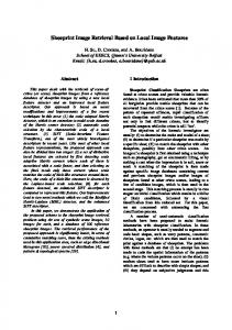
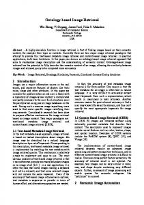
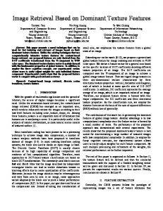
and asymmetrical response profiles in order to achieve minimum uncertainty in both spatial localization and spatial frequency (Coggins and Jain, 1985; Daugman, 1985). In the article we propose Gabor filters for extracting texture features needed to characterize images in a database. Then such features can be effectively used as information in content based image retrieval (CBIR) applications. Images are retrieved based on the similarities feature, where features of the query specification are compared with features from the image database to determine which images match similarly with given features. Typically, most CBIR systems use shape, color and texture parameters and perform separate classification for those features (Smeulders et al., 2000; Chora´s, 2003). A typical scheme of a CBIR system is presented in Fig. 1. We propose to use Gabor filtration and Gabor texture features since texture usually distinctively describes images of most classes (Conners and Harlow, 1980; Ma and Manjunath, 1996). First, we perform image normalization so that extracted salient points and texture features will not change due to contrast and illumination changes. Then multichannel Gabor filtering and the idea of hierarchical image representation are presented. A salient (characteristic) point extraction algorithm is described next. Furthermore, we compute texture features only in a neighborhood of salient points. Features are also based on Gabor filtration. The article is concluded with feature representation, a similarity measure, conclusions and remarks on future work. A general diagram of our CBIR solution based on Gabor filtration and Gabor texture features is shown in Fig. 2.

T. Andrysiak and M. Chora´s

472

later in our method, depends on the illumination variance in the image. Therefore, in order to achieve illumination and contrast invariance, we normalize the image. Let I (x, y) denote the gray value at the pixel (x, y) in the M × M image matrix I, E and V be the estimated mean and illumination variance in the image I, respectively, and f (x, y) stand for the normalized graylevel value at the pixel (x, y). For all the pixels in the image I, the normalization process is defined as follows:  ⎧ ⎪ ⎪ V0 (I (x, y)−E)2 ⎪ ⎪ E + if I (x, y) > Th, ⎪ ⎨ 0 V f (x, y) =  ⎪ ⎪ 2 ⎪ ⎪ V0 (I (x, y)−E) ⎪ ⎩E0 − otherwise, V (1) where E0 and V0 are the desired mean and variance values, respectively, and E and V are the computed mean and variance in the given image, described by Fig. 1. Typical CBIR system scheme (Chora´s, 2003).

E=

M−1 M−1 1   I (x, y), M 2 x=0 y=0

(2)

V =

M−1 M−1 1   (I (x, y) − E)2 , M 2 x=0 y=0

(3)

2. Image Grayscale Normalization Before filtering the image, we normalize all its regions to a certain mean and variance. Normalization is performed to remove the effects of sensor noise and gray level deformation. Moreover, the extraction of salient points, performed

respectively. In our case, E0 = 100 and V0 = 100.

Fig. 2. General scheme of our CBIR solution.

Image retrieval based on hierarchical Gabor filters

473

3. Binarization and Coordinate Normalization

4.1. Gabor Filters

In the next step, we perform binarization and coordinate size normalization. The binary image is given by

b (x, y) =

⎧ ⎨ 1

if I (x, y) > th,

⎩ 0

otherwise,

(4)

where th is a threshold value, such as the intensity of the first minimum that occurs after the maximum value of the intensity histogram.

The two-dimensional Gabor filter family can be represented as a complex sinusoidal signal modulated by a Gaussian function (window). Specifically, a twodimensional Gabor filter ψ (x, y; σ, λ, θk ) can be formulated as follows:   2πxθk i , (9) ψ (x, y; σ, λ, θk ) = g (x, y; σ) exp λ and



x2 + γ 2 yθ2k g (x, y; σ) = exp − θk 2σ 2

 (10)

Moreover, in order to achieve the invariance of geometrical transformations (translation, rotation and scaling), we change the [x, y] coordinate system into an invariant system of [x , y  ] coordinates such as

is a Gaussian function, where

[x , y  , 1]

and σ is the standard deviation of the Gaussian envelope along the x- and y-dimensions, and λ and θk are the wavelength and orientation, respectively. The parameter γ is usually equal to 0.5. Since the spatial aspect ratio γ is constant, we do not use it as a Gabor filter parameter. The rotation of the x–y plane by an angle θk will result in a Gabor filter at the orientation θk . The angle θk is defined by π (13) θk = (k − 1) n for k = 1, 2, . . . , n and n ∈ N, where n denotes the number of orientations. The odd and even components of the above signal are as follows:   2πxθk ψe (x, y; σ, λ, θk ) = g (x, y; σ) cos , (14) λ   2πxθk ψo (x, y; σ, λ, θk ) = g (x, y; σ) sin , (15) λ

⎡

1 ⎢ = [x, y, 1] ⎣ 0 −I

⎤⎡ 0 1/σx ⎥⎢ 0 ⎦⎣ 0 0 1

0 1 −J ⎡

cos β ⎢ × ⎣ − sin β 0

0 1/σy 0

sin β cos β 0

⎤ 0 ⎥ 0 ⎦ 1

⎤ 0 ⎥ 0 ⎦ , (5) 1

where I=

m10 , m00 

σx =

J=

m20 − I, σy = m00

m01 , m00 

m02 − J, m00

(6)

(7)

for moments of order p + q defined as  mpq =

xp y q b (x, y) dx dy.

(8)

4. Hierarchical Image Representation As a result of basic preprocessing operations described in Sections 2 and 3, we obtain images that are resistant to image transformations and illumination distortions. Such normalized images become the input of multichannel Gabor filtration and hierarchical image representation. This approach enables us to practically implement the idea of bottom-up processing and feature extraction (Jain et al., 1997; Namuduri et al., 1994).

xθk = x cos(θk ) + y sin(θk ),

(11)

yθk = −x sin(θk ) + y cos(θk ),

(12)

where ψe and ψo are the even-symmetric and oddsymmetric Gabor filters, respectively. The parameter λ is the wavelength and 1/λ the spatial frequency of the harmonic factor cos (2πxθk /λ) or sin (2πxθk /λ). The ratio σ/λ determines the spatial frequency bandwidth of Gabor filters. The half-response spatial frequency bandwidth (in octaves) and the ratio σ/λ are related in accordance with  ⎛ ⎞ ln(2) σ π + λ 2 ⎠,  (16) b = log2 ⎝ ln(2) σ π − λ 2 1 σ = λ π



ln(2) 2b + 1 , 2 2b − 1

where σ/λ is constant and equal to 0.56.

(17)

T. Andrysiak and M. Chora´s

474 4.2. Multichannel Gabor Filtration In order to extract features of the retrieved objects, we used multiresolution Gabor filtration tuned to four selected filter orientations. The computations are made for each of the filter orientations and for each filter resolution (Andrysiak and Chora´s, 2003; Namuduri et al., 1994). The input image f (x, y) is convolved with a 2-D Gabor filter ψo (x, y; σ, λ, θk ) to obtain the Gabor image response: Φ (x, y; σ, λ, θk )  = f (η, ζ) ψo (x − η, y − ζ; σ, λ, θk ) dη dζ. (18) By utilizing the recursive filtering method, we can generate a set of hierarchical filters starting from the odd component of the Gabor filter. The input image is filtered by each of these filters to generate the responses of a family of Gabor filters. The recursive filtering method, when applied to a directional 2D odd Gabor filter, increases the resolution of the filter, while maintaining its directional selectivity (Young et al., 2002). The algorithm for implementing a recursive filtering method of computing multiresolution responses starts with the odd component of the Gabor filter ψo (x, y; σ, λ, θk ) tuned to the following steps: Step 1. Convolve the image with the filter ψo (x,y; σ, λ, θk ) for k = 1, . . . , 4 and obtain the set Φ(j) .   Step 2. Convolve the response Φ(j) with the Gaussian  (j−1)  g(x, y; σ) and obtain Φ .  (j−1)  with the GausStep 3. Convolve the response Φ √   sian g(x, y; 2σ) and obtain Φ(j−2) .   Step 4. Resample the response Φ(j−2) of the resolution level j − 2. Step 5. Substitute j = j − 2 and go to Step 2. Terminate the algorithm for the lowest resolution level. The responses generated by this algorithm correspond to multiple resolutions as shown below: Φ(j) = f (x, y) ∗ ψo(j) (x, y; σ, λ, θk ) ,   √ Φ(j−1) = f (x, y) ∗ ψo(j−1) x, y; 2σ, 2λ, θk ,

(19) (20)

Φ(j−2) = f (x, y) ∗ ψo(j−2) (x, y; 2σ, 4λ, θk ) , (21)   √ Φ(j−3) = f (x, y) ∗ ψo(j−3) x, y; 2 2σ, 8λ, θk . (22) In order to simplify the filtration, the consecutive steps are implemented as the convolution of filtration parameters with the Gaussian function. A realization of this process and the selection of parameters are presented in Appendix.

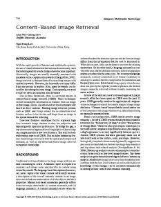
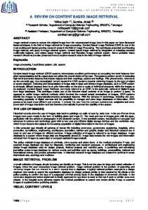
The results of Gabor hierarchical filtering using the recursive method are shown in Figs. 3, 4 and 6. The responses of the Gabor filter at three different resolutions λ for the hierarchical representation of the image “plate” are shown in Fig. 3. The results and the idea of hierarchical feature extraction are presented in Fig. 4. The number of extracted features increases as the resolution changes. The number of extracted features is considerably higher in the right image. The responses of the Gabor filter at three different resolutions λ for the hierarchical representation of the image “blocks" are shown in Fig. 6. 4.3. Gabor Filter Design In our CBIR method, we use odd and even component pairs of Gabor filters with the quadrature phase relationship. Each pair of the Gabor filters is tuned to a specific band of spatial frequency and orientation. There are some important points to note in selecting the channel parameters σ, λ and θk . Four values of orientation are used: 0, π/4, π/2, 3π/4. In our experiments for each orientation we select three spatial frequencies. This gives a total of 12 Gabor channels (4 orientations combined with 3 frequencies).

5. Extraction of Salient Points Our algorithm for the extraction of salient (characteristic) points is based on the hierarchical representation of images resulting from consecutive filtration according to the algorithm presented in Section 3.2. The process starts from the lowest level of hierarchical image representation. Those are images that contain only general features. Such an image is presented in Fig. 4 (left). The consecutive steps of the algorithm are as follows:   Step 1. We divide the image Φ(j−3) into non-overlapping blocks b(k, l) of the size n × n. Step 2. For each of those blocks we compute the variance V (k, l). Step 3. We look for p points of the maximum variance that characterize p blocks bmax (k, l) of  (j−3) of the image, where p corresponds to Φ the number of the desired salient points. Blocks of maximum variance contain considerable illumination changes which usually correspond to the contours of objects within the image.   Step 4. For each block bmax (k, l) from the Φ(j−3) level we look for the corresponding block b(r, s) of the size  2n in the next resolution level  2n × image Φ(j−2) .

Image retrieval based on hierarchical Gabor filters

475

Fig. 3. Results of recursive filtering tuned to different resolutions.

Fig. 4. Selected images of different resolutions. The increasing number of extracted features is presented (from left to right).

  Step 5. We divide each block b(r, s) from the Φ(j−2) level into 5 parts according to Fig. 5. Then we compute the variances {Vi }, i = 1, 2, . . . , 5, for newly created blocks.

6. Texture Feature Extraction Based on Gabor Filters

Fig. 5. Salient point extraction algorithm—Step 5.

Step 6. We look for the maximum variance Vmax = max {Vi } , i

Step 7. Substitute j = j + 1 and go to Step 4. Terminate the algorithm if the highest resolution level is achieved. Then in each block bmax (k, l) of the maximum variance we look for a point with the maximum value of the filter response. The found point becomes the extracted salient point. The results of the consecutive steps of this algorithm for different resolutions are presented in Fig. 7. Finally, the result for the sample image “blocks” is shown in Fig. 8.

(23)

which unambiguously characterizes the appropriate block bmax (k, l).

Each texture in the image is characterized by a given localized spatial frequency or a narrow range of dominant localized spatial frequencies that differ significantly from dominant frequencies of other textures. Gabor filters encode the textured images into multiple narrow frequency and orientation channels (Petkov, 1995).

T. Andrysiak and M. Chora´s

476

Fig. 6. Results of recursive filtering tuned to different resolutions.

Fig. 7. Consecutive steps of hierarchical salient point extraction.

Fig. 8. Result of the salient point extraction algorithm.

Image retrieval based on hierarchical Gabor filters

477

The filter responses that result from the application of a filter bank of Gabor filters can be used directly as texture features. Three different preferred spatial frequencies and four different preferred orientations were used, resulting in a bank of 12 Gabor filters. Moreover, other features such as Gabor Energy and complex moments covered in the next subsections are computed.

The simplest idea to obtain other features than just filter responses is to apply a threshold to the Gabor filter results. The motivation for such an approach is the analogy to the function of simple cells which can be modeled by a linear weighted spatial summation, characterized by Gabor weighting functions and followed by a half-wave rectification (Petkov and Kruizinga, 1997). The thresholded Gabor features are computed as follows: To (x, y; σ, λ, θk ) = χ (Φo (x, y; σ, λ, θk )) ,

(24)

Te (x, y; σ, λ, θk ) = χ (Φe (x, y; σ, λ, θk )) ,

(25)

 χ (z) =

0 z

for z < 0, for z ≥ 0,

(26)

Cm,n (x, y)  m n ˆ (x, y; u, v) du dv, (29) = (u − iv) (u − iv) P m, n ∈ N, where u=

1 cos(Θ), λ

u=

1 sin(Θ), λ

ˆ (x, y; u, v) = P (x, y; λ, θk ) P

6.2. Gabor Energy Features The Gabor Energy feature is a combination of symmetric and asymmetric Gabor filter results. Gabor Energy is related to the model of a specific type of selective neuron orientation in the primary visual cortex called the complex cell (Field, 1987). Gabor Energy is given by E (x, y; σ, λ, θk )  = T2o (x, y; σ, λ, θk ) + T2e (x, y; σ, λ, θk ), (27) where To (x, y; σ, λ, θk ) and Te (x, y; σ, λ, θk ) are the threshold responses of the linear symmetric and asymmetric Gabor filters, respectively. The Gabor Energy feature is also closely related to the local power spectrum. Local power spectrum features are obtained using the same filter bank as in the computations of Gabor Energy features: (28)

(30) (31)

for σ = const, and where m+n (m, n ∈ N) is the order of the complex moment, which is related to the number of dominant orientations in the texture. It can be proven that the complex moments Cm,n of odd orders are zero and that all complex moments for which m = n are real. Furthermore, ∗ Cm,n = Cn,m ,

and Φo (x, y; σ, λ, θk ) and Φe (x, y; σ, λ, θk ) are the odd and even components of Gabor filter responses, respectively.

P (x, y; σ, λ, θk ) = E2 (x, y; σ, λ, θk ) .

Several authors proposed to use the real and imaginary parts of complex moments of the local power spectrum as features (Bigun and Buf, 1994; 1995). Such parameters are interesting since they tell us if there are any dominant orientations in the texture (Kruizinga and Petkov, 1999a). Complex moments of the local power spectrum are defined by

6.1. Thresholded Gabor Features

where

6.3. Complex Moment Features

(32)

so that it is sufficient to consider only the Cm,n s with m ≤ n (Kruizinga and Petkov, 1999b). In our experiments we use filters with both symmetric and asymmetric Gabor functions. Two banks, each containing 12 filters (with 4 orientations and 3 spatial frequencies), are used, one comprising the symmetric and the other the asymmetric filters. From this set we select only the nonzero real and imaginary parts.

7. Similarity Measure After calculating Gabor texture features, we obtain several feature vectors: • the vector of symmetric and assymetric Gabor filter responses R(x, y; σ, λ, θk ):  R = Φo (x, y; σ, λ, θk ), Φe (x, y; σ, λ, θk ) , (33) • the vector of thresholded and energy Gabor features T (x, y; σ, λ, θk ) given by  T = To (x, y; σ, λ, θk ), Te (x, y; σ, λ, θk ), E(x, y; σ, λ, θk ), P (x, y; σ, λ, θk ) , (34)

T. Andrysiak and M. Chora´s

478 • the vector of the complex moments C, cf. Eqn. (29). Finally, we construct the final feature vector F V (x, y; σ, λ, θk ), which will be later used in the image retrieval similarity measure. The final feature vector is given by F V (x, y; σ, λ, θk )  = R(x, y; σ, λ, θk ), T (x, y; σ, λ, θk ), C . (35) After the normalization of each component in the vector F V (x, y; σ, λ, θk ), we calculate the similarity of a query image Q and an image D from the database, defined as  d(Q)(D) (R, T, C) = d(Q)(D) , (36) p p

where d(Q)(D) p

! ! ! ! = !Rp(Q) − Rp(D) ! + !Tp(Q) − Tp(D) ! ! ! +!Cp(Q) − Cp(D) !, (37)

and p is the number of the extracted salient points.

8. Conclusions and Future Work Gabor filters are efficiently used in many applications of computer science. In the article we have proposed a multichannel Gabor filtration scheme used for the detection of salient points and the extraction of texture features for image retrieval applications. In the neighborhood of salient points we calculate texture features which are also Gabor based and we store them in the feature vector F V (x, y; σ, λ, θk ). Our CBIR solution is based on Gabor filtration and therefore we also calculated texture features related to Gabor filters. Those features are straightforward to compute, and together with Gabor filter responses ensure a sufficient image representation. For an image database of small post-stamps we achieved results comparable to the known CBIR systems such as Blobworld , since the texture distinctively describes most post-stamp classes. However, other features are needed in order to effectively retrieve images from large databases containing images of various types. Such features may contain color and shape features as shown in Fig. 1. Therefore, we work on adding global and local color histograms and parameters connected with the shapes of objects within images. In the extracted salient points we create Regions of Interest (ROIs) in which we calculate color histograms and Zernike moments (Chora´s et al., 2005). Then all the extracted features can be efficiently used as queries in the automatic content based image retrieval (CBIR) system based on multichannel Gabor filtration and hierarchical image representation.

References Andrysiak T. and Chora´s M. (2003): Hierarchical object recognition using Gabor wavelets. — Proc. Comput. Recogn. Syst., KOSYR, Miłków, Poland, pp. 271–278. Bigün J. and du Buf J.M.H. (1994): N-folded symmetries by complex moments in Gabor space. — IEEE Trans. Pattern Anal. Mach. Intell., Vol. 16, No. 1, pp. 80–87. Bigün J. and du Buf J.M.H. (1995): Symmetry interpretation of complex moments and the local power spectrum. — Vis. Commun. Image Represent., Vol. 6, No 2, pp. 154–163. Chen Y. and Wang J.Z. (2002): A region-based fuzzy feature matching approach to content-based image retrieval. — IEEE Trans. Pattern Anal. Machine Intell., Vol. 24, No. 9, pp. 1252–1269. Chora´s R. (2003): Content-based retrieval using color, texture, and shape information, In: Progress in Pattern Recognition, Speech and Image Analysis (Alberto Sanfeliu, José Ruiz-Shulcloper, Eds.). — Berlin: Springer, pp. 619–626. Chora´s R. (2004): Fuzzy processing technique for content based image retrieval, In: Artificial Intelligence and Soft Computing (L. Rutkowski et al., Eds.). — Springer, LNAI, Vol. 3070, pp. 448–451. Chora´s R., Andrysiak T. and Chora´s M. (2005): Content based image retrieval technique, In: Computer Recognition Systems (M. Kurzy´nski et al., Eds.). — Springer, pp. 371–379. Coggins J.M. and Jain A.K. (1985): A spatial texture approach to texture analysis. — Pattern Recogn. Lett., Vol. 3, No. 7, pp. 195–203. Conners R. and Harlow C. (1980): A theoretical comparison of texture algorithms. — IEEE Trans. Pattern Anal. Mach. Intell., Vol. 2, No. 3, pp. 204–222. Daugman J.G. (1985): Uncertainty relation for resolution in space, spatial frequency, and orientation optimized by twodimensional visual cortical filters. — J. Opt. Soc. Amer. A, Vol. 2, No 7, pp. 1160–1169. Daugman J.G. (1988): Complete Discrete 2D Gabor Transforms by Neural Networks for Image Analysis and Compression. — IEEE Trans. Acoust., Speech Signal Process., Vol. 36, No. 7, pp. 1169–1179. Daugman J.G. (1998): Recognizing persons by their iris patterns, In: Biometrics: Personal Identification in Networked Society (A.K. Jain, R. Bolle and S. Pankanti, Eds.). — Kluwer Academic Publishers, pp. 103–121. Field D.J. (1987): Relations between the statistics of natural images and the response properties of cortical cells. — J. Optic. Soc. Amer., Vol. 4, No 12, pp. 2379–2394. Fogel I. and Sagi D. (1989): Gabor filters as texture discriminator. — Biol. Cybern., Vol. 61, pp. 103–113. Gabor D. (1946): Theory of communication. — J. Instit. Electr. Eng., Vol. 93, pp. 429–457. Hammamoto Y. (1999): A Gabor filter-based method for fingerprint identification, In: Intelligent Biometric Techniques in Fingerprint and Face Recognition (L.C. Jain, U. Halici et al., Eds.). — CRC Press, pp. 137–151.

Image retrieval based on hierarchical Gabor filters

479

Jain A. and Farrokhnia F. (1991): Unsupervised texture segmentation using Gabor filters. — Pattern Recogn., Vol. 24, No. 12, pp. 1167–1186.

Spitzer H. and Hochstei S. (1985): A complex-cell receptive-field model. — J. Neurosci., Vol. 53, No. 5, pp. 1266–1286.

Jain A., Ratha N. and Lakshmanan S. (1997): Object detection using Gabor filters. — Pattern Recogn., Vol. 30, No 2, pp. 295–309.

Su Y.M. and Wang J.F. (2003): A novel stroke extraction method for Chinese characters using Gabor filters. — Pattern Recogn., Vol. 36, No. 3, pp. 635–647.

Kruizinga P. and Petkov N. (1999): Non-linear operator for oriented texture. — IEEE Trans. Image Process., Vol. 8, No. 10, pp. 1395–1407.

Turner M.R. (1990): Texture discrimination by Gabor functions. — Biolog. Cybern., Vol. 55, No 1, pp. 55–73.

Kruizinga P., Petkov N. and Grigorescu S.E. (1999): Comparison of texture features based on Gabor filters. — Proc. Int. Conf. Image Analysis and Processing, IAP, Venice, Italy, pp. 142–147.

Weldon T.P., Higgins W.E. and Dunn D.F. (1996): Efficient Gabor filter design for texture segmentation. — Pattern Recogn., Vol. 29, No. 12, pp. 2005–2015.

Lee T. (1996): Image representation using 2D Gabor wavelets. — IEEE Trans. Pattern Anal. Mach. Intell., Vol. 18, No. 10, pp. 959–971.

Wiskott L., Fellous J.M., Kruger N. and Malsburg C.V.D. (1997): Face recognition by elastic bunch graph matching. — IEEE Trans. Pattern Anal. Mach. Intell., Vol. 19, No. 7, pp. 775–779.

Liu C. and Wechsler H. (2001): A Gabor feature classifier for face recognition. — Proc. IEEE Int. Conf. Computer Vision, Vancouver, Canada, pp. 270–275. Ma W.Y. and Manjunath B.S. (1996): Texture Features and Learning Similarity. — Proc. IEEE Conf. Computer Vision and Pattern Recognition, San Francisco, USA, pp. 425– 430. Malik J. and Perona P. (1990): Preattentive texture discrimination with early vision mechanisms. — J. Optic. Soc. Amer., A, Vol. 7, No 5, pp. 923–932. Manjunath B.S. and Ma W.Y. (1996): Texture Features for Browsing and Retrieval of Image Data. — IEEE Trans. Pattern Anal. Mach. Intell., Vol. 18, No 8, pp. 837–842. Marcelja S. (1980): Mathematical description of the responses of simple cortical cells. — J. Optic. Soc. Amer., Vol. 2, No 7, pp. 1297–1300. Mehrotra R., Namuduri K. and Ranganathan N. (1992): Gabor filter-based edge detection. — Pattern Recogn., Vol. 25, No 12, pp. 1479–1494. Namuduri K.R, Mehrotra R. and Ranganathan N. (1994): Efficient computation of Gabor filter based multiresolution responses. — Pattern Recogn., Vol. 27, No 7, pp. 925–938. Petkov N. and Kruizinga P. (1997): Computational models of visual neurons specialised in the detection of periodic and aperiodic oriented visual stimuli: Bar and grating cells. — Biolog. Cybern., Vol. 76, No 2, pp. 83–96. Petkov N. (1995): Biologically motivated computationally intensive approaches to image pattern recognition. — Future Gener. Comput. Syst., Vol. 11, pp. 451–465. Porat M. and Zeevi Y.Y. (1988): The generalized Gabor scheme of image representation in biological and machine vision. — IEEE Trans. Pattern Anal. Mach. Intell., Vol. 10, No 4, pp. 452–468. Smeulders A.W.M., Worring M., Gupta A. and Jain R. (2000): Content-based image retrieval at the end of the early years. — IEEE Trans. Pattern Anal. Mach. Intell., Vol. 22, No. 12, pp. 1349–1380.

Young I.T, Vliet van L.J. and Ginkel van M. (2002): Recursive Gabor filtering. — IEEE Trans. Signal Process., Vol. 50, No. 11.

Appendix Let Ψo (x, y; σ, λ) represent 2D odd Gabor filter with the parameters σ, λ, and let g (x, y; σ) represent a 2D symmetric Gaussian function with the parameter σ. The convolution is given by Ψo (x, y; σ, λ) ∗ g (x, y; σ) +∞  +∞  = Ψo (x − δ, y − ρ; σ, λ)g (x, y; σ) dδ dρ, −∞ −∞

where ‘*’ denotes the convolution operation and σ and ρ are dummy variables for integration. Computing the convolution on the right-hand side of the above equation, we get Ψo (x, y; σ, λ) ∗ g (x, y; σ) "  # +∞  +∞  2 2 (x − δ) + γ 2 (y − ρ) = exp − 2σ 2 −∞ −∞



 2π (x − δ + y − ρ) λ $  2 % δ + γ 2 ρ2 × exp − dδ dρ 2σ 2 × sin

T. Andrysiak and M. Chora´s

480 +∞ +∞ "  & '#  x2 −2xδ+2δ 2 +γ 2 y 2 −2yρ+2ρ2 exp − = 2σ 2 −∞−∞

× sin

π

$

λ

= exp −

 (2x − 2δ + 2y − 2ρ) dδ dρ 2

2 2

x +γ y 4σ 2

× cos

"  & '# x2 −24xδ+4δ 2 +γ 2 y 2 −4yρ+4ρ2 exp − 4σ 2

−∞−∞

× sin

π

$

λ

= exp −



(x + y) + (x − 2δ + y − 2ρ) dδ dρ 2

2 2

x +γ y 4σ 2

+∞  +∞ 

× −∞ −∞

π

2

2

(x − 2δ) + γ 2 (y − 2ρ) 4σ 2

$   π  π × sin (x + y) cos (x − 2δ + y − 2ρ) λ λ  π (x + y) + cos λ % π (x − 2δ + y − 2ρ) dδ dρ × sin λ



"  # +∞  +∞  2 2 (x − 2δ) + γ 2 (y − 2ρ) exp − × 4σ 2 × sin

#

(x − 2δ + y − 2ρ)

λ $ 2 %  π x + γ 2y2 + exp − (x + y) cos 4σ 2 λ

−∞ −∞

%

" 

exp −

"  # +∞  +∞  2 2 (x − 2δ) + γ 2 (y − 2ρ) exp − × 4σ 2 −∞ −∞

%

+∞ +∞ 

×

%  π x2 + γ 2 y 2 (x + y) sin = exp − 4σ 2 λ $

π

λ

 (x − 2δ + y − 2ρ) dδ dρ.

The first integral involving the Gabor even filter in the above equation is constant, while the second integral involving the Gabor odd filter is equal to zero. Hence the above convolution is reduced to Ψo (x, y; σ, λ) ∗ g (x, y; σ)  2   π x + γ 2y2 = A exp − (x + y) , sin 4σ 2 λ where A is a constant. Finally, the convolution √of these'two filters results in & a Gabor odd filter Ψo x, y; 2σ, 2λ .