Image Segmentation with A Bounding Box Prior - Welcome to TU ...

Image Segmentation with A Bounding Box Prior Victor Lempitsky, Pushmeet Kohli, Carsten Rother, Toby Sharp Microsoft Research Cambridge

Abstract User-provided object bounding box is a simple and popular interaction paradigm considered by many existing interactive image segmentation frameworks. However, these frameworks tend to exploit the provided bounding box merely to exclude its exterior from consideration and sometimes to initialize the energy minimization. In this paper, we discuss how the bounding box can be further used to impose a powerful topological prior, which prevents the solution from excessive shrinking and ensures that the user-provided box bounds the segmentation in a sufficiently tight way. The prior is expressed using hard constraints incorporated into the global energy minimization framework leading to an NP-hard integer program. We then investigate the possible optimization strategies including linear relaxation as well as a new graph cut algorithm called pinpointing. The latter can be used either as a rounding method for the fractional LP solution, which is provably better than thresholding-based rounding, or as a fast standalone heuristic. We evaluate the proposed algorithms on a publicly available dataset, and demonstrate the practical benefits of the new prior both qualitatively and quantitatively.

1. Introduction Foreground/background segmentation of photographs is an inherently ambiguous problem. Practical systems rely on user interactions and provide a way to combine such interactions with the low-level cues, such as color distributions and contrast edges observed in the image. The objective is then to build a system that can segment images as accurately as possible with as little user intervention as possible. Among several types of user interaction paradigms that have been investigated and implemented, the bounding box interaction is, arguably, the most natural and one of the most economical in terms of the amount of user interaction. Bounding box is a concept that is intuitive to users, and it takes only two mouse clicks to specify it. But what information does the user-specified bounding box provide about the segmentation problem? First, it restricts the attention of the segmentation process

without the prior

with the prior

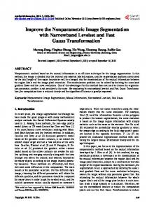
Figure 1. Our tightness prior. The segmentation on the left computed with graph cut is consistent with the low level image cues, yet inconsistent with the user input (in yellow) being too loose for this bounding box. By minimizing the same graph cut energy under a set of constraints, our method computes the segmentation that fits the bounding box in a sufficiently tight way, obtaining a better result (right).

to the interior of the bounding box. This property is easy to incorporate into any algorithm, as one can simply assign all exterior pixels to the ‘background’ class. The second property is much harder to incorporate or even to formalize. Informally, it can be expressed as: “users provide bounding boxes that are not too loose, but are sufficiently tight”, or in other words, the desired segmentation should have parts that are sufficiently close to each of the sides of the bounding box. Developing a new segmentation framework that is capable of enforcing such tightness is the goal of this paper. Figure 1 illustrates the importance of this property. To some extent, this tightness property can be taken into account by methods based on local curve evolution such as geodesic active contours [5]. A method of this type can initialize the ’foreground’ region to contain the full bounding box and then perform its energy-driven shrinking. Here, the hope is that the local minimum found by the process would likely to be tight in the above sense, as the shrinking process would not go too far. Such an approach, however, suffers from two significant drawbacks. First, this is just a hope and there are no guarantees that the energy optimization would not shrink the segmentation excessively. Secondly, local optimization processes are notorious for getting stuck

at poor local minima, which are suboptimal with respect to the low-level cues. Our framework takes a different approach and avoids the pitfalls of local curve evolution. Instead, it employs global optimization techniques, namely convex continuous optimization and graph cuts, which we briefly review in Section 2. In summary, the key aspects and contributions of the paper are: • It proposes a formalization of the notion of tightness. As a result, the task of segmentation under the tightness prior can be written down as an integer program (IP). Within this program, the objective incorporates low-level cues such as consistency with color distribution of segments and edges in the image, while the set of constraints enforce the tightness of the segmentation with respect to the provided bounding box (Section 3). • The paper investigates techniques for the approximate solution of the above-mentioned IP. We first consider a continuous relaxation of the integer program, which can be solved exactly by an iterative application of a linear programming solver. We then present a new approximate graph cut-based algorithm called pinpointing, which may be used either as a rounding procedure for the relaxed solution or as a fast standalone heuristic for the original IP (Section 4). • The paper evaluates the proposed algorithms on a publicly-available dataset of segmentation problems with ground truth [1]. The practical benefits of having the tightness prior are demonstrated both qualitatively and quantitatively (Section 5). Apart from these contributions, we believe that the developed optimization techniques have broader applicability than the task addressed in the paper. E.g. the pinpointing algorithm can be applied to multiview reconstruction with silhouette constraints in a similar way to [9]. We comment on this broader perspective within the discussion in section 6.

2. Related Work on Global Optimization Energy minimization is used within most recently proposed segmentation frameworks. Graph cut-based minimization for image segmentation, first introduced by by Boykov and Jolly [3], gained particular popularity because it can handle energies that unify edge-contrast and image appearance cues, while obtaining the global optimum of such energies at interactive speed. Let us consider an image B as a set of pixels p ∈ B, and denote with cp the vector describing the appearance of a pixel p (e.g. the RGB color). Assume that the segmentation of the image is given by its 0−1 labeling x ∈ 2B , where individual pixel labels xp take the value 1 for foreground and 0 for background. Then, a typical graph cut segmentation

energy [6, 3] can be written as: X X E(x) = U p ·xp + V pq ·|xp −xq |, p∈B

xp ∈ {0, 1} ,

{p,q}∈E

(1) where E is a set of pairs of adjacent pixels. Here, U p are the so-called unary potentials that encode the preference of each pixel to be either foreground or the background, while the pairwise potentials V pq ≥ 0 are used to enforce the smoothness of the solution and to align its boundary with image edges. The global minima of (1) can be found in polynomial time by reducing the problem to a st-mincut/maxflow on a pixel graph [6]. The same global minima may be obtained using convex continuous optimization by relaxing the integrality constraint xp ∈ {0, 1} to xp ∈ [0, 1] and thresholding the solution of the resulting linear problem at any value between 0 and 1 [13]. Furthermore, tackling the optimization problem (1) with the convex continuous optimization allows to replace the pairwise terms with the total variation terms [11]. These may have the same effect of aligning the boundaries of the segmentation with contrast edges while not suffering from the metrication artifacts. This improvement is however orthogonal to the issues we address in this paper, so we stick with the pairwise terms as in (1). Optimization problems of the form (1) and their totalvariation counterparts defined on pixel/voxel grids have been used not only for image segmentation, but also for several other computer vision tasks including multiview reconstruction. Thus, Kolev and Cremers [9] demonstrated how non-local constraints (which in their case corresponded to silhouette rays) can be incorporated into a global optimization framework leading to an integer program that can be relaxed to a convex continuous one. We took inspiration from their framework and investigate a similar approach to the image segmentation problem. Finally, recently and independently, Nowozin and Lampert [12] have presented a framework for segmentation under connectivity constraint. Our framework shares a lot of similarities with [12], in particular in the way it relaxes an NP-hard integer problem and solves the resulting LP. At the same time, the relatively easier prior that we handle, different kind of LP relaxation we employ, and the new graph-cut based pinpointing algorithm that we propose lead to considerably smaller computational burden in our case. Thus, for average-sized images our algorithms work with individual pixels, while [12] have to perform super-pixelization.

3. Tackling Tightness Given a user-specified bounding box, we can restrict our attention to its interior, so that in the rest of the paper we will assume that the image B corresponds to the subimage inside the bounding box. While the minimization of (1)

a. Definitions b. Strongly tight c. Non-tight d. Weakly tight Figure 2. Tightness of shapes: the outer rectangles are userprovided, the transparent colour rectangles are the margins, the shapes are in transparent black, red and blue dashed lines correspond to long and short crossing paths. In (b,c,d) we show examples of a strongly tight, a non-tight, and a weakly but not strongly tight shapes. In (c,d) the non-intersecting crossing paths are shown.

would make the segmentation consistent with foreground and background appearance models and the contrast edges in the image, it will not enforce any kind of tightness of the bounding box, e.g. it may not prevent the foreground region from excessive shrinking. In this subsection, we discuss how the bounding box tightness prior can be enforced. To formalize this “sufficient tightness” we introduce the notion of left, right, top, and bottom margins, which are subboxes of B adjacent to its edges (Figure 2a). As will become clear, the margin thickness (i.e. the height of top and bottom margins and the width of left and right margins) reflects the degree of tightness that is expected from the userprovided bounding box. We also consider the middle box that is a part of the bounding box between the margins. The tightness in our approach is introduced via the concept of the crossing path, that we define in two ways: Definition 1: A short crossing path is a curve inside the middle box M, that has endpoints on the opposite sides of M. Definition 2: A long crossing path is a curve inside the bounding box B, that either has endpoints on the left and the right sides and goes between (does not intersect) the top and the bottom margins, or has endpoints on the top and the bottom sides of B and goes between the left and the right margins. We then introduce the two classes of tight shapes: Definition 3: A shape x is strongly tight if it intersects all short crossing paths. Definition 4: A shape x is weakly tight if it intersects all long crossing paths. As each long crossing path is a superset of a short one, it is clear that all strongly tight shapes are weakly tight as well (but not vice versa – see Figure 2d). For strongly tight shapes, the following important property holds: Corollary 1: A shape x is strongly tight if and only if its intersection with the middle box has a connected component touching all four sides of the middle box (see [10] for the proof). This property links tightness with connectivity and en-

sures that our notion of tightness makes sense, as, informally speaking, the strong tightness turns out to be equivalent to having a connected chunk of foreground that comes close to each of the sides of the bounding box. Note, that the connectivity property is, in general, hard to incorporate into global optimization frameworks [15, 12]. Weak tightness, on the other hand, has a nice monotonicity property: Corollary 2: when the thickness of all four margins is increased (or kept the same), the new set of weakly tight shapes is a superset of the old one (see [10] for the proof). The rest of our derivations hold for both strong and weak tightness, so we will in general simply use the terms tightness and crossing path (which in each case should be understood either as strong tightness and short crossing path or as weak tightness and long crossing path). As we are interested in discrete shapes defined on pixel grids, we consider the set Γ of all 4-connected crossing paths on a raster. Then, by requiring that each 4-connected path C ∈ Γ has at least one foreground pixel, we can add the tightness prior into the graph cut framework arriving at the following integer program (IP): X X U p ·xp + V pq ·|xp − xq | → min (2a) p∈B

{p,q}∈E

s.t.

∀p

∀C ∈ Γ

xp ∈ {0, 1} X xp ≥ 1

(2b) (2c)

p∈C

The constraints (2c) ensures that each of the paths C ∈ Γ has at least one foreground pixel. Any feasible solution of (2) is tight (for the case of strong tightness, a feasible solution has an 8-connected component intersecting all four sides of the middle box). We now discuss different strategies for solving this IP.

4. Optimization 4.1. Convex Continuous Relaxation Solving the IP (2) is an NP-hard problem. In fact, it is equivalent to the minimization of a non-submodular function. Thus, approximations have to be derived. One natural idea is to relax the integrality constraints (2b), replacing xp ∈ {0, 1} with xp ∈ [0, 1]. The resulting program may be turned into a linear program (LP) in a standard way: X

U p ·xp +

p∈B

X

V pq ·ypq → min

(3a)

{p,q}∈E

s.t.

∀p

∀C ∈ Γ

0 ≤ xp ≤ 1 X xp ≥ 1

(3b) (3c)

p∈C

∀ {p, q} ∈ E

ypq ≥ xp − xq , ypq ≥ xq − xp

(3d)

4.2. Pinpointing Algorithm This program still cannot be handled by a generalpurpose LP solver, as the number of constraints specified in (3c) is combinatorial (exponential in the size of the bounding box B). This is not however as hard a problem as it may seem at the first glance, as these constraints can be tackled iteratively. To do that we solve a sequence of LP problems that have the form (3), with the only modification that each time we consider a subset Γ0 ⊂ Γ of all crossing paths in the constraint set (3c). The algorithm proceeds as follows: 1. In the first iteration, the subset of path constraints is empty (Γ0 = ∅), i.e. all constraints (3c) are inactive. 2. After the LP from the previous iteration is solved, we pick a group of crossing paths from Γ \ Γ0 that have the corresponding constraints (3c) violated by more than some small tolerance  and activate these constraints, adding this group to Γ0 . This step is detailed below. 3. After this, the LP (3) with the new set Γ0 is solved and the iterations proceed until constraints of all crossing paths in the full set Γ are satisfied (within tolerance ) and no further constraints may be added in step 2. On the termination of the algorithm, the solution of the LP with the constraint set Γ0 is -feasible with respect to the full constraint set Γ. We have observed that for tolerance  = 0, the process may run for a long time. However, even for small  > 0 (e.g.  = 0.05), the process converged within few iterations (typically less than five). The size of the set of activated constraints Γ0 is typically linear in the largest dimension of the bounding box B and hence exponentially smaller than the full set Γ. Note that the effect of introducing a small finite tolerance  is negligible in comparison with the effect of approximating the original IP program (2) with its linear relaxation (3). We now explain our method for selecting the group of crossing path constraints in step 2 of the algorithm above. Let us denote with xcur the solution of the LP in the previous iteration. We P first pick the crossing path C1 ∈ Γ with the smallest sum p∈C1 xcur We then find the crossing p . P path C2 with the smallest sum p∈C2 xcur that does not p intersect with C1 . In general, we continue picking the paths P Ci with the smallest sum p∈Ci xcur that do not intersect p Fi−1 with the previous paths (Ci ∩ j=1 Cj = ∅). Each time the optimal path can be easily found with two runs of Dijkstra algorithm (from top to bottom and from left to right). From the non-intersection requirement, it can be seen that at most n − 2d constraints may be picked at a time, where n is the largest dimension of B and d is the margin thickness. As discussed P above, we stop picking constraints as far as the sum p∈Ci xcur exceeds 1 − . All the picked constraints p are then added to the set Γ0 .

The output of the linear program (3) is a fractional solution xLP ∈ [0; 1]B , which needs to be rounded to the integer solution xIP ∈ {0, 1}B . The simplest and popular choice (see e.g. [9]) for the rounding procedure is to threshold the fractional solution at some threshold τ : ( 1, if xLP > τ, p IP . The selected threshold τ needs xp = 0, otherwise to be small enough to ensure that the rounded solution satisfies all crossing path constraints (2c) of the IP. Among this set the largest possible τ should be selected to achieve the lowest objective (2a). Thresholding-based rounding strategy is completely agnostic about the objective function (2a) of the IP. By taking the objective into account better rounding strategies may be developed. Below, we present a new rounding algorithm called pinpointing that is provably better than the thresholding-based rounding. Pinpointing (Figure 3) is based on graph cut minimization and approximates the IP (2) with another integer program: X p∈B

U p ·xp +

X

V pq ·|xp − xq | → min

(4a)

{p,q}∈E

s.t.

∀p

∀p ∈ Π

xp ∈ {0, 1}

(4b)

xp = 1

(4c)

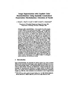
Here, the pinpoint set Π contains pixels that are hardassigned to the foreground. Note, that unlike the original NP-hard integer program (2) the new program (4) corresponds to the traditional graph cut energy that can be minimized exactly and efficiently in polynomial time using stmincut/maxflow [6, 3]. The pinpointing procedure capitalizes on this efficiency by constructing the pinpoint set Π in a way that the optimal solution of the new program (4) is a feasible solution for the original program (2). The intuition is that since the two programs share the same objective and integrality constraints, the optimal solution of (4) will be a reasonable approximation to the optimal solution of (2). To construct the pinpointing set Π, the pinpointing algorithm assumes that it is given a real-valued priority map P (p) → R, which may be e.g. the fractional solution computed using linear programming. Then, during the first stage, the pinpointing set is greedily expanded according to the priority map until the optimal solution of (4) satisfies all path constraints (2c) of the original IP. During the second stage, the pixels are greedily removed from Π until the obtained pinpointing set Π is minimal in a sense that exclusion of any of its members makes the optimal solution of (4) infeasible with respect to the path constraints (2c) of the original IP.

a) Solution with Π = ∅

b) After the 1st pixel is added to Π

c) After expansion stage

d) After shrinking stage

Figure 3. The pinpointing algorithm adjusts the set Π (pixels denoted with yellow crosses) to make the optimal solution of the graph cut program (4) satisfy all crossing path constraints. The set Π is first greedily expanded (a-c), then greedily shrunk (d). See text for further details of the algorithm.

In more detail, the first stage starts with an empty set Π (Figure 3a). At each step i, the current pinpointing set Πi is considered and the optimal solution xi of the program (4) is computed via graph cut. Then, the algorithm checks whether the crossing paths that do not intersect the foreground pixels exist. If there are no such paths, then the expansion stage is terminated as the optimal solution of (4) is the feasible solution of the original IP (2). Otherwise, the active set Ai that contains pixels belonging to any of this paths is considered (Figure 3a - red). We then chose the pixel ri ∈ Ai with the highest value of the priority map P (ri ) and add this pixel to the pinpointing set Πi+1 = Πi ∪ {ri }, after which the iterations proceed (Figure 3b) until xi satisfies all path constraints (2c) (Figure 3c). During the second stage, the algorithm goes through the pinpointing set Π in the order the pixels were added into it. It then tries to remove each of the pixels p in Π out of the set and compute the optimal solution of the program (4) with the set Π \ p. If the resulting solution remains feasible with respect to the original IP (2), then the change is accepted and the pixel is removed from the pinpointing set. As a result, the minimal set Π is obtained (Figure 3d). Note, that the energy of the solution goes down or stays the same with each exclusion step, since the optimization domain in (4) becomes larger. Two computational tricks ensure the fast performance of pinpointing. First, the st-mincut/maxflow problems corresponding to the integer programs (4) that are solved during subsequent steps of the algorithm are highly correlated (in fact, they differ by the weight of a single edge). Therefore, the dynamic reuse of the search trees and flow [8] in the maxflow algorithm [4] makes the individual stmincut/maxflow computations extremely cheap, so that the time spent on all graph cut computations is only few times larger than the time required to solve a single graph cut from scratch. Secondly, the problems of checking the feasibility of the integer solution with respect to the original IP (2) and determining the active set A can be solved extremely cheaply using the connected component analysis (floodfill operations). Pinpointing as rounding procedure. The pinpointing algorithm can be used to round the fractional solution of the

IP. To do this, one can simply use this fractional solution as a priority map. Importantly, the following theoretical guarantee about such rounding scheme can be given: Corollary 3 (pinpointing gives lower energy than thresholding): Let xf be any fractional solution of (2). Let xτ be a feasible integer solution of (2) obtained by thresholding xf with some threshold τ . Let xP P be a solution obtained by pinpointing with the priopity map xf . Then, E(xP P ) ≤ E(xτ ). (The proof is given in [10].) Pinpointing with other Priority Maps. Importantly, pinpointing does not require its priority map to be computed by solving the LP or any other approximation to the integer program. Simpler and/or cheaper to compute priority maps can be used instead. Perhaps the simplest choice for the priority map P (p) that was surprisingly efficient in our experiments, are the unary terms: P (p) = −U (p). Another possible choice that has awareness about both the unary and the pairwise terms in the objective are the min-marginals [8] (or more precisely minus 1-min-marginals). While of heuristic nature, resulting algorithms are often as efficient in terms of the energy of the obtained solution as pinpointing based on the LP solution, and are very often more efficient than thresholding the LP solution.

5. Experiments We have evaluated our methods on the GrabCut dataset of 50 natural images with ground truth segmentations [1]. In the dataset, each image comes with a bounding box that has been automatically computed from the ground truth1 . To the best of our knowledge, our work is the first to report the performance of any algorithms on this dataset with the bounding box inputs. Note that the error rates reported here are not comparable with those reported in previous works for the same dataset with the trimap input. Unary and pairwise terms. We used the 8-connected edge set E and standard ways to compute the unary and pair1 We have also modified the bounding boxes on few images, wherever the bounding box touched the boundary, while the object did not. This modification benefited all algorithms equally, and without it the baseline GrabCut algorithm [14] was not applicable to one of the images. New bounding boxes are available at [1].

Input

Unary terms

Ground truth

GraphCut

LP-Threshold LP-Pinpoint

Unary-PP.

MinMarg.-PP.

E = −0.042 E = −0.055 E = −0.039 E = −0.039 Figure 4. Results of the methods on the relatively easy (top) and one of the hardest (bottom) images from the GrabCut dataset. Note how adding the tightness prior improves the results and also enforces connectedness in the bottom row. For the second problem, we give the energy values obtained with the last 4 methods.

wise terms. Pairwise terms were computed as: V pq =

1 · exp (−α − β||C p − C q ||) , ||p − q||

(5)

where C p and C q are the pixel RGB color vectors, || · || is a Euclidean norm, and the constants were set as α = 8, β = 80/ max{p,q}∈E ||Cp − Cq ||. Following [2, 14] we used Gaussian mixtures to compute the unary terms. To do this, we first fit the Gaussian mixture model (with 5 components) to the color vectors of the strip of 10 pixels around the bounding box. We then evaluated the probability of pixels inside the bounding box under this initial background GMM. Finally, we fit the foreground Gaussian mixture model GM Mf to the 33% pixels with the smallest probability and the final background mixture model GM Mb to the 33% of the pixels with the largest probability joined together with the strip pixels. The unary terms were then defined as:
U p = λ log P (C p |GM Mb ) − log P (C p |GM Mf ) , (6) where the λ parameter was set to 10−6 . Finally, we modified the unary values for the pixels adjacent to the boundary of the bounding box in the following way. Wherever the side of the bounding box did not touch the image boundary,

the unary terms of all pixels along these side were set to +∞, ensuring that the foreground segment does not touch that side of the bounding box. Unless specified otherwise, we worked with the weak definition of tightness and we set the thickness of all four margins to d=0.06 of the largest bounding box dimension. With this choice of thickness, all ground truth segmentations were tight. Experiment 1. Relative performance. The following algorithms were run on the dataset: • Unary-Threshold: Thresholding of the unary terms (xp were set to 1 wherever U p were negative). This was included in the evaluation to give a rough idea about the quality of the unary terms. • GraphCut: Solving (1) using standard graph cut without taking the tightness prior into account. • LP-Threshold: Solving the IP (2) by solving the linear program (3) and rounding using thresholding. • LP-Pinpoint: Solving the IP (2) by solving the linear program (3) and rounding using pinpointing. • Unary-Pinpoint: Solving the IP (2) by pinpointing with the priority map based on unary terms (P (p) = −U p ). • MinMarginal-Pinpoint: Solving the IP (2) by pinpoint-

Method Error-50 Error-22 Optim.Rank Unary-Threshold 12.7 15.0 – GraphCut 6.7 8.9 – LP-Threshold 5.4 5.9 2.82 LP-Pinpoint 5.0 5.1 1.32 Unary-Pinpoint 5.2 5.6 2.77 MinMarginal-Pinpoint 5.4 6.0 3.09 Table 1. Experiment 1 results. Error rates (in %) and the optimization performance on the GrabCut dataset demonstrating an improvement gained by the enforcement of the tightness prior. See text for further discussion.

ing with minus 1-MinMarginals [7] as the priority map. After running the algorithms on the dataset, we have computed the error rates as the percentage of mislabeled pixels inside the bounding box. We then averaged these numbers over all images in the dataset (’Error-50’ column on Table 1). We have also observed that on 28 images the graph cut solution was already tight, so that all methods except Unary-Threshold returned identical result. Therefore, we have also computed the error rates over the other 22 images, where the methods performed differently (’Error-22’ column on Table 1). A considerable decrease in error rates in both columns suggested the usefulness of the tightness prior. Finally, we compared the energies of segmentations produced by the last 4 methods, which solve the same integer program (2). Qualitatively, we have observed that the differences were typically small, with Unary-Pinpoint and LP-Pinpoint methods typically obtaining the lowest energies and all 4 algorithms obtaining visually very similar results on the majority of examples (such as the top row on Figure 4). On the few hardest images (such as the bottom row on Figure 4) the LP-Pinpoint algorithm typically performed the best, while other pinpointing algorithms were pinpointing points too greedily. To get the quantitative summary of these observations, we ranked the algorithms according to the energy of obtained solutions from 1 = lowest energy (good) to 4 = highest energy (bad). When methods produced identical solutions they were ranked with the same rank. We then averaged the ranks over the 22 images, and gave the result in the 3rd column of Table 1. Interestingly, these numeric ranks based on obtained energies are in accordance with the relative performance of methods in terms of error rates, which serves as an evidence that the integer program (2) is a good model for the segmentation task. Experiment 2. Iterative process. In [14], Rother et al. suggested the GrabCut framework, which interleaved the segmentation graph cut steps with the unary terms reestimation: each time the segmentation is computed, the foreground and the background Gaussian mixtures are refitted to the new foreground and background segments, and the

Method GrabCut-GC GrabCut-GC GrabCut-Pinpoint GrabCut-Pinpoint

Initialization InitFullBox InitThirds InitFullBox InitThirds

Error

Error

λ=10−6

λ=2·10−6

8.9 5.9 8.2 3.7

7.2 5.1 7.3 4.5

Table 2. Experiment 2 results. The error rates of the results obtained by our method on the GrabCut dataset demonstrate the power of the sufficient tightness prior in the iterative GrabCut framework. We show the average error rates on the entire dataset for different algorithms (GrabCut with and without prior), different initializations, and different smoothness parameter λ. The top row thus corresponds to the algorithm in [14], and the bottom row to our best algorithm.

Figure 6. Error rates (in %) as the function of the margin thickness (as a multiple of the largest bounding box dimension) on the GrabCut dataset for GrabCut-GC and GrabCut-Pinpoint (with ’InitThirds’ initialization). A graceful degradation of GrabCutPinpoint for overly large thickness can be seen.

iterations continue. We have experimented with this procedure running it for 5 iterations. The two algorithms were compared here: • GrabCut-GC, a conventional GrabCut algorithm [14] that uses standard graph cut minimization (1) for all segmentation steps. • GrabCut-Pinpoint, a new algorithm that enforces the tightness prior on each segmentation step. For the sake of speed, the Unary-Pinpoint algorithm was used to solve the IP (2). We have also compared the two ways to initialize mixture models: as was used in the Experiment 1 (InitThirds) and as suggested in [14], where the foreground mixture is initially fitted to the whole interior of the user-provided bounding box and the background mixture is fitted to the strip outside it (InitFullBox). The results, which demonstrate the advantage of having the tightness prior, are given in Table 2 and Figure 5. As the accuracy of the conventional GrabCut (GrabCut-GC) peaked at the value of λ about twice as large as we were using for the experiments, Table 2 reports the results for double smoothness as well. As an aside, note that the new initialization heuristics (“InitThirds”) works better, no matter whether GrabCut-GC or GrabCut-Pinpoint was used. We would also like to note that the primitive error measure that

Figure 5. Results of iterated GrabCut with (right/bottom) and without (left/top) the tightness prior on the images from the GrabCut dataset, where the prior had the largest effect (more results are given in [10]). The prior improves the segmentation accuracy and predictability. Each image represents the interior of the provided bounding box with the superimposed segmentation boundary.

we used might not convey the actual improvement from our prior, e.g. it does not reflect the improvements in topology of segmentations. Finally, Figure 6 demonstrates the degree of sensitivity of our method to the choice of the thickness d of the margins. While excessively small margins result in high rates, choosing excessively large margins result in graceful degradation of the performance. Strong vs. weak tightness. In our experiments, the strong tightness led to error rates very similar to those obtained with the weak tightness. The error rate for GrabCutPinpoint, “InitThirds” was the same (3.7%). Computation speed. In our current implementation, the use of a general purpose linear solver for the program (3) makes our LP-based algorithms slow (minutes per image). However, the GPU implementation of a specially designed interior point method may bring a significant speed-up. The Unary-Pinpoint algorithm is already quite fast being only 1 to 15 (typically 1–4) times slower than a conventional GraphCut algorithm for the same image.

6. Discussion We have introduced a new bounding-box based prior for interactive image segmentation and demonstrated how segmentation tasks under this prior can be formulated as integer programs. We have also developed new optimization approaches for approximate solution of these NP-hard problems. We believe that the developed optimization techniques can find application within a broader spectrum of computer vision applications (e.g. other global constraints for image segmentation or silhouette constraints in multiview stereo).

References [1] Grabcut dataset: http://tinyurl.com/grabcut. [2] A. Blake, C. Rother, M. Brown, P. P´erez, and P. H. S. Torr. Interactive image segmentation using an adaptive gmmrf model. In ECCV (1), pages 428–441, 2004. [3] Y. Boykov and M.-P. Jolly. Interactive graph cuts for optimal boundary and region segmentation of objects in n-d images. In ICCV, pages 105–112, 2001. [4] Y. Boykov and V. Kolmogorov. An experimental comparison of mincut/max-flow algorithms for energy minimization in vision. IEEE Trans. Pattern Anal. Mach. Intell., 26(9):1124–1137, 2004. [5] V. Caselles, R. Kimmel, and G. Sapiro. Geodesic active contours. In ICCV, pages 694–699, 1995. [6] D. M. Greig, B. T. Porteous, and A. H. Seheult. Exact maximum a posteriori estimation for binary images. Journal of the Royal Statistical Society, 51(2), 1989. [7] P. Kohli and P. H. S. Torr. Effciently solving dynamic markov random fields using graph cuts. In ICCV, pages 922–929, 2005. [8] P. Kohli and P. H. S. Torr. Measuring uncertainty in graph cut solutions - efficiently computing min-marginal energies using dynamic graph cuts. In ECCV (2), 2006. [9] K. Kolev and D. Cremers. Integration of multiview stereo and silhouettes via convex functionals on convex domains. In ECCV (1), pages 752–765, 2008. [10] V. Lempitsky, P. Kohli, C. Rother, and T. Sharp. Image segmentation with a bounding box prior. In MSR-TR-2009-85. [11] M. Nikolova, S. Esedoglu, and T. F. Chan. Algorithms for finding global minimizers of image segmentation and denoising models. SIAM Journal of Applied Mathematics, 66(5):1632–1648, 2006. [12] S. Nowozin and C. Lampert. Global connectivity potentials for random field models. In CVPR, 2008. [13] C. H. Papadimitriou and K. Steiglitz. Combinatorial Optimization: Algorithms and Complexity. Prentice-Hall. [14] C. Rother, V. Kolmogorov, and A. Blake. ”GrabCut”: interactive foreground extraction using iterated graph cuts. ACM Trans. Graph., 23(3):309–314, 2004. [15] S. Vicente, V. Kolmogorov, and C. Rother. Graph cut based image segmentation with connectivity priors. In CVPR, 2008.