Image sharpening by morphological "ltering - Pattern Recognition ...

Pattern Recognition 33 (2000) 997}1012

Image sharpening by morphological "ltering J.G.M. Schavemaker!,*, M.J.T. Reinders", J.J. Gerbrands", E. Backer" !Electro-Optical Systems, TNO Physics and Electronics Laboratory, P.O. Box 96864, 2509 JG The Hague, Netherlands "Information and Communication Theory Group, Department of Electrical Engineering, Faculty of Information Technology and Systems, Delft University of Technology, P.O. Box 5031, 2600 GA Delft, Netherlands Received 10 December 1998; received in revised form 2 May 1999; accepted 23 June 1999

Abstract This paper introduces a class of iterative morphological image operators with applications to sharpen digitized gray-scale images. It is proved that all image operators using a concave structuring function have sharpening properties. By using a Laplacian property, we introduce the underlying partial di!erential equation that governs this class of iterative image operators. The parameters of the operator can be determined on the basis of an estimation of the amount of blur present in the image. For discrete implementations of the operator class it is shown that operators using a parabolic structuring function have an e$cient implementation and isotropic sharpening behavior. ( 2000 Pattern Recognition Society. Published by Elsevier Science Ltd. All rights reserved. Keywords: Image sharpening; Mathematical morphology; Flat and quadratic structuring functions; Slope transform; Partial di!erential equations; Document processing

1. Introduction Kramer et al. [1] de"ne a non-linear transformation for sharpening digitized gray-scale images. The transformation replaces the gray value at a pixel by either the minimum or the maximum of the gray values in its neighborhood, the choice depending on which one is closer in value to the original gray value. They show that after a "nite number of iterative applications, the resulting image stabilizes, that is, every pixel becomes either a local maximum or a local minimum. Osher and Rudin derive the same property for shock "lters for image enhancement [2]. They use partial di!erential equations and their discretizations and show that solutions of the equations satisfy a local maximum and minimum principle. The advantages of the above non-linear transformation for sharpening digitized gray-scale images are

* Corresponding author. Tel.: #31-70-374-0860; fax: #3170-374-0654. E-mail address: [email protected] (J.G.M. Schavemaker)

multiple. The transformation is fast, computationally e$cient, and easy to implement (local maximum and minimum operator). Furthermore, the transformation reduces the number of gray values present in the original image, and does not su!er from overshooting at edges, as opposed to methods based on the use of standard (linear) "lters. These last methods as for instance, unsharp masking [3}5] or the Laplacian operator [6], have the tendency to amplify noise and need clipping or scaling to make the resultant pixels span the interval [0, 255]. Verbeek et al., on the other hand, show in Ref. [7] that the non-linear transformation, denoted as dynamic-front operator, has edge-sharpening properties, but their dynamic front operator is not iterative. Practical applications of the sharpening transformation have been reported by Lester et al. [8], Den Hartog [9], and by Schavemaker [10]. In this paper, it is shown that the transformation introduced by Kramer et al. actually is an instance of a class of morphological image operators that all have sharpening properties, which class can be characterized by a partial di!erential equation. Based on this generalization we show that there is another kind of imagesharpening operator that outperforms the original

0031-3203/00/$20.00 ( 2000 Pattern Recognition Society. Published by Elsevier Science Ltd. All rights reserved. PII: S 0 0 3 1 - 3 2 0 3 ( 9 9 ) 0 0 1 6 0 - 0

998

J.G.M. Schavemaker et al. / Pattern Recognition 33 (2000) 997}1012

transformation introduced by Kramer et al. in both algorithm order complexity as well as isotropic sharpening behavior.

Secondly, the quadratic structuring functions (QSF) as introduced by van den Boomgaard [12]:

AB

qo(A)(x)"oq(A) 2. Introduction to mathematical morphology In mathematical morphology [11], the transformation that replaces the gray value at a pixel by the (weighted) maximum of the gray values in its neighborhood is known as the gray-scale dilation image operator: ( f = g) (x)" S [ f (u)#g(x!u)] (1) u|R2 in which function f (x), f : x3R2 C f (x)3R is the original image, and g(x), g : x3R2 C g(x)3R is the structuring function implicitly de"ning the weighted neighborhood. Similarly, the transformation that replaces the gray value at a pixel by the (weighted) minimum of the gray values in its neighborhood is known as the gray-scale erosion image operator: (2) ( f >g) (x)" R [ f (u)!g(u!x)]. 6|R2 Note that the dilation operator is extensive: ( f=g) (x)*f (x), and the erosion operator is anti-extensive: ( f>g)(x))f (x). Fig. 2(a) gives a one-dimensional example of the dilation and erosion image operator.

G

co(x)"

xTx)o2,

!R, xTx'o2.

1 qo(x)"! xTx. 2o

(3)

(5)

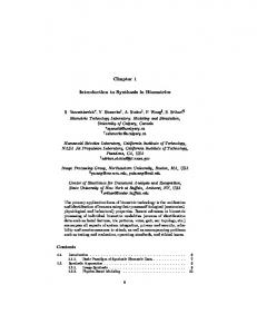
For both types of a structuring function, the parameter o determines the size (or scale) of the structuring function. Fig. 1 gives a two-dimensional example of a #at and parabolic structuring function. In practical applications of mathematical morphology, the use of a #at structuring function is widespread [1,13,14]. Its popularity stems from the fact that the gray-scale dilation and erosion operators using a #at structuring function are easy to implement (local maximum and minimum "lter) and result in fast algorithms. Van den Boomgaard et al. [15] prove for the class of quadratic structuring functions that: f Any quadratic structuring function is dimensionally decomposable with respect to dilation: ∀A : &R, a, b : ( f = qo(A)) (x)

A

In the remainder of this paper, we focus on the following two structuring functions. Firstly, the yat structuring functions as used by Kramer et al. in their original de"nition of the image-sharpening operator:

(4)

where A is a 2]2 positive-de"nite symmetric matrix. Taking the unity matrix for A yields the symmetric twodimensional parabolic structuring function:

A A BB A A B BB

" f = qo RT

3. Structuring functions

0,

x 1 "! xTA~1x, o 2o

=qo RT

a 0 0 0

0 0

0 b

R

R

(x).

(6)

f The general class of quadratic structuring functions contains the subclass of structuring functions that are rotationally symmetric: qo(x)"!(1/2o)xTx, i.e. those

Fig. 1. Parabolic and #at structuring function: (a) parabolic structuring function qo(x)"!(1/2o)xTx, and (b) #at structuring function co(x).


structuring functions for which

A B

A"

1 0 0 1

.

4. Image-sharpening operator class

(7)

These properties allow for very e$cient algorithms for implementing the parabolic dilation operator, that have been shown to be independent of the size of the structuring function [15]. Given these scalable structuring functions go(x) we rede"ne the dilation and erosion operator: F^(x, o)"( f = go) (x),

(8)

F>(x, o)"( f > go)(x),

(9)

F (x, 0)"F^(x, 0)"F>(x, 0)"f (x).

(10)

The functions F^(x, o) and F>(x, o) are the morphological scale-space notations for the gray-scale dilation and gray-scale erosion image operators with structuring function go(x) [12]. The parameter o is the scale parameter of the morphological scale space. The original function is f (x) and x is the position. The operators ( f = g) (x) and ( f > g) (x) are the dilation and erosion operators as de"ned in Eq. (1) and (2). Note that one can derive a scalable structuring function from any concave structuring function g(x) by means of umbral scaling:

AB

go(x)"og

x . o

(11)

For example, the scalable parabolic structuring function qo(x) can be derived from the structuring function q(x)"!1 xTx: 2

AB

qo(x)"oq

x o xTx 1 "! "! xTx. o 2 o2 2o

(12)

The scalable #at structuring function co(x) can be derived from structuring function,

G

c(x)"

0,

xTx)1,

(13)

!R, xTx'1

in a similar manner:

AB

G

x co(x)"oc " o

G

0,

0,

xTx )1 o2

!R,

xTx '1 o2

xTx)o2,

"

!R, xTx'o2.

999

(14)

In this section we give a de"nition of the image-sharpening operator class in terms of gray-scale dilation image operators and gray-scale erosion image operators; it is an extension of Kramer's original de"nition. Furthermore, we prove that iterative applications of the sharpening operator using a concave structuring function have sharpening properties. 4.1. Image-sharpening operator class dexnition First, we rephrase the original transformation de"ned by Kramer et al. in the framework of mathematical morphology: e[ f ](x, o)

G

F^(x, o), F^(x, o)!F(x, 0)(F(x, 0)!F>(x, o),

" F>(x, o), F^(x, o)!F(x, 0)'F(x, 0)!F>(x, o), F (x, 0), otherwise. (15)

This image-operator class is parameterized by the structuring function go(x). If we take a #at structuring function co(x) as the structuring function go(x), then the image-sharpening operator equals the original de"nition of Kramer et al. with one modi"cation: Kramer et al. did not consider the special case where F^(x, o)! F (x, 0) equals F (x, 0)!F>(x, o). In that case, the image-sharpening operator as de"ned by Kramer et al. behaves as the dilation operator (F^(x, o)). In case of a single-slope signal (∀x : +2 f"0), the application of the operator as de"ned by Kramer et al. results in a translation of the original signal, whereas this new de"nition preserves the original signal. Fig. 2(b) gives a one-dimensional example of an application of the sharpening operator. Fig. 3 gives a two-dimensional example of an application of the sharpening operator on a scanned part of a utility map. Note that Eq. (15) de"nes one application of the sharpening operator. In practical applications, however, it is generally bene"cial to use multiple iterative applications of the operator with a small structuring function. The size of the structuring function determines the sharpening speed. If we use a sharpening operator with a large structuring function, we require less iterative applications than with a small structuring function, but we lose small details in the resulting image, see for example Fig. 4. In general, this choice is a trade-o! between speed and accuracy. Repeated application of the sharpening operator for a "xed scale of the structuring function will sharpen the image until a "xed point is reached, i.e. application of the operator will no longer alter the image. In the following, we show that this repeated sharpening behavior is controlled by a partial di!erential equation

1000


Fig. 2. (a) One-dimensional example of gray-scale dilation image operator = and gray-scale erosion image operator >. (b) Imagesharpening operator E[ f ] takes values from f = g or f > g.

Fig. 3. One application of the image-sharpening operator E[ f ]. Shown are the original image f, the dilation f = g, the erosion f > g, and the sharpening result E[ f ].

Fig. 4. Choice of the size of a structuring function, i.e. speed versus accuracy. (a) Part of a scanned utility map (400 dpi). (b) Result of the image-sharpening operator with a 3]3 #at structuring function: three iterative applications were necessary to achieve a sharp image. (c) Result after one iteration of the image-sharpening operator with a 7]7 #at structuring function: the decimal dot is merged with the digit.


(PDE). By examining this PDE optimal structuring functions can be derived. 4.2. Laplacian properties for one-dimensional continuous functions In this section it is shown that the sign of the Laplacian of function f (x) at position x determines whether f (x) is going to be dilated or eroded by the sharpening operator. With this important property of the sharpening operator the PDE will be derived. For the sake of explanation, it is shown for one-dimensional continuous functions only, but it can simply be generalized to two-dimensional functions, which is shown in Section 4.3. In the remainder of this paper a concave function is de"ned as follows: a function g(x), g : x 3 R C g(x) 3 R is concave if for all x , x 3 R the line connecting the 0 1 points (x , g(x )) and (x , g(x )) is below the function 0 0 1 1 g(x). A function is convex when it is not concave. For any one-dimensional symmetric (go(x)"go(!x)) concave structuring function go(x), go : x 3 R C go(x) 3 R and o 3 R`, the following properties of the image-sharpening operator class hold: E[ f ](x, o)'f (x) if +2f (x)(0,

(16)

E[ f ](x, o)(f (x) if +2f (x)'0,

(17)

E[ f ](x, o)"f (x) if +2f (x)"0,

(18)

where +2f (x) is the Laplacian of function f (x). Before proving properties (16)}(18), we introduce the slope transform S[ f ](w). For symmetric concave structuring

1001

functions go(x), we have that for both cases x'0 and increasing x, as well as for x(0 and decreasing x, that the derivative of go(x), +go(x) is a decreasing function. This implies that the intercept of a tangent line of go(x) in x with the functional axis (y-axis) is an increasing function for increasing x'0 as well as for decreasing x(0, as depicted in Fig. 5(a). The intercept function is known as the slope transform S[go] (w) of function go(x), see Fig. 5(a). The slope transform was introduced by Dorst and Van den Boomgaard [16,17] and is closely related to the A-transform as introduced by Maragos [18]. The slope transform is a function of slope w and is set valued. Because our structuring functions are concave, the slope transform of these functions is single valued. To prove Eq. (16), we consider a function f (x) with +2f (x)(0 for a certain value of x, x . To determine the dilation and 1 erosion value of function f (x) at x , we use the 1 hit property of the dilation image operator and the hit property of the erosion image operator. The hit property of the dilation image operator can be explained with Fig. 5(b). To determine the dilation value d at 0 x (( f = go) (x )) we place the inverse structuring function 1 1 !go (x) above function f (x) in such a way that the origin of the inverse structuring function !go(x) is located at (x , #R). After that, we shift the origin downwards (i.e. 1 we translate it along the functional axis) until it hits the function f (x) (let us say in (x , f (x )). The function value a a of the thus translated origin sets the new dilation value of function f (x) at x . Now assume that we take the interval 1 [x , x ] so small that we may linearly approximate f (x) 0 1 within this interval. Note that because +f (0, +f (x )'+f (x ). Let us further assume that we have a b

Fig. 5. (a) Intercept with the functional axis (slope transform of go at +go). (b) Hit property of gray-scale dilation and gray-scale erosion image operator.

1002


taken the scale of the structuring function su$ciently small (pB0) that the hit position is within the above interval, i.e. x (x (x . Then the gradient of the struc0 a 1 turing function is equal to the gradient of function f (x) at x"x : a +f (x )"+!go(x !x )"+go(x !x ). a 1 a a 1

(19)

The dilation value d at x can now simply be derived 0 1 from the slope transform, i.e. d "S[go](+f (x )). The 0 a same applies for the hit property of the erosion image operator. In that case, we use structuring function go(x) and place its origin below function f (x), at x , i.e. 1 (x ,!R) and shift it upwards. Consequently, the ero1 sion value d at x equals d "S[go](+f (x ). Because 1 1 1 b +2f (x )(0, we have 1 +f (x )'+f (x ) a b

(20)

and S[go](+f (x ))(S[go](+f (x )), a b

(21)

we derive that d (d . This sets the image-sharpening 0 1 operator value at x to the dilation value F^(x , o) and 1 1 proves property (16). Property (17) is proved by the duality of the erosion image operator. Property (18) is proven by the fact that when +2f (x)"0, the sharpening operator equals F(x, 0)"f (x). 4.3. Laplacian properties for two-dimensional continuous functions Generalization of Eqs. (16) and (17) to the two-dimensional case is not trivial because the Laplacian is de"ned as L2f L2f +2f (x)" # . Lx2 Lx2 0 1

(22)

Now there are two cases for which +2f (x)(0: Case 1:

L2f L2f (0 and (0. Lx2 Lx2 0 1

Case 2:

L2f L2f L2f L2f (0, '0 and ' Lx2 Lx2 Lx2 Lx2 0 1 0 1

(and vice versa for x and x ) 0 1

(23)

(24)

L2f L2f '0 and '0. Lx2 Lx2 0 1

Case 4:

L2f L2f L2f L2f '0, (0 and ' Lx2 Lx2 Lx2 Lx2 0 1 0 1

(and vice versa for x and x ). 0 1

4.4. Sharpening properties for a one-dimensional edge model To demonstrate the sharpening properties of the image-sharpening operator, we construct an analytical edge model. Let the original edge be represented by function i(x), i : x 3 R C i(x) 3 R. Suppose further that the recording of the original edge can be modeled by a linear system. Hence, the recorded edge function f (x), f : x 3 R C f (x) 3 R is given by f (x)"i (x)*h (x),

i (x)" (25)

(26)

(27)

where * is the convolution operator and h (x) is the point spread function (PSF), h : x 3 R C h (x) 3 R. Function f (x) is depicted in Fig. 6(c). Let us assume a symmetrical lens, i.e. h (x)"h(!x), with "nite aperture, i.e. h (x)"0 for x!a and x'a for some a 3 N. Moreover, h(x)*0 and h(x) is a decreasing function for increasing and decreasing x. Point spread function h (x) is depicted in Fig. 6(b). Suppose the original edge is an ideal step edge, that is, i(x) is the unit step function:

G

and two cases for which +2f (x)'0: Case 3:

For case 1, f (x) is concave at position x. When we use a rotational-symmetric concave structuring function go(x) for the sharpening operator, the dilation value at position x is closer in value to the original gray value than the erosion value. Therefore, property (16) still holds for two-dimensional continuous functions; its proof is analogous to the proof for one-dimensional continuous functions. For case 3, f (x) is convex. When we again use a rotational-symmetric concave structuring function go(x) for the sharpening operator the value of the erosion at position x is closer to the original gray value than the dilation value. As a consequence, property (17) also holds for two-dimensional continuous functions; its proof is analogous to the proof for one-dimensional continuous functions. For cases 2 and 4, L2f /Lx2 and L2f /Lx2 do not have 0 1 the same sign, hence f (x) is neither convex nor concave in x. In these cases it will also depend on the values L2f /Lx2 0 and L2f /Lx2 whether the dilation value or the erosion 1 value is chosen as the resulting value after the application of the sharpening operator. The "nal choice is made on the basis of the highest partial second-order derivative value, giving the lowest slope transform value in x or x . 0 1

1,

x)0,

0,

x'0.

(28)

Function i(x) is shown in Fig. 6(a). When convolving with h(x), note that +f (x)(0 for x 3 [!a, a] and, as h(x) is decreasing and symmetric, that +2f (x)(0 for x3[!a, 0), +2f (x)'0 for x 3 (0, a], and +2f (x)"0 for x"0. The image-sharpening operator E[ f ] only changes function f (x) at points x that have +2f (x)O0.


1003

Fig. 6. (a) Original picture i(x). (b) Point spread function h(x). (c) Blurred version f (x) of original picture i(x). (d) One iteration of the image-sharpening operator.

Consider the interval [!a, 0) in which points x have +2f (x)(0, as depicted in Fig. 6(c). This interval represents a concave part of the function f (x). One application of the image-sharpening operator with a concave structuring function go(x) results in F^(x, o) at this interval, as shown in Fig. 6(d). As F^(x, o)'f (x) is true at this interval (Eq. (16)), the interval at which points x have +2F^(x, o)(0, i.e. [!b, 0), becomes smaller than the original interval [!a, 0), at which +2f (x)(0. Furthermore, because we use a concave structuring function go(x), F^(x, o) is also concave at the interval [!a, 0) (proved in Ref. [16]). As a consequence, repeated applications of the image-sharpening operator on the interval [!a, 0) result in an interval [!a, !c), with !b(c(0, at which all points x have function values equal to the maximum function value in the interval [!a, 0), i.e. f (!a). The same holds for the convex interval (0, a] with points x having +2f (x)'0. In this case, repeated applications of the image-sharpening operator result in an interval (c, a], with 0(c(b, at which all points x have function values equal to the minimum function value in the interval (0, a], i.e. f (a). After a "nite number of applications of the image-sharpening operator, the blurred function f (x) is sharpened to the original picture i (x). The exact number of needed sharpening applications is derived in Section 4.6. 4.5. Sharpening properties for a two-dimensional edge model If the structuring function go(x) is rotationally symmetric and concave, the sharpening properties of the sharpening operator also hold for edges with arbitrary orientations in two-dimensional images. For two-dimensional

oriented edges, the sharpening is perpendicular to the direction of the edge, and can be considered to be a collection of one-dimensional sharpening applications, as discussed in Section 4.4. Fig. 7(a) gives a visual example. This property can be derived using the hit property of the dilation and erosion operator and the fact that the structuring function is rotationally symmetric, (see Figs. 7(b) and (c)). The isophotes of Fig. 7(a) run parallel to the edge. As such, when we sharpen the edge, the structuring function will hit the edge in a point for which the line through the point and the origin of the structuring function is perpendicular to the direction of the edge, (see Fig. 7(b)). This implies that sharpening a point x on the edge only requires function values of points on the line that runs through x and is perpendicular to the edge. As a result, sharpening two-dimensional oriented edges can be considered to be a collection of one-dimensional sharpening applications, as shown in Fig. 7(c). Both the #at and parabolic structuring function are rotationally symmetric. However, discrete approximations of small #at structuring functions are not isotropic and can cause anisotropic sharpening behavior, as discussed in Section 8.1. 4.6. Number of iterative applications In this section we derive the number of iterative applications of the sharpening operator necessary to sharpen one edge. The number of applications depends on the PSF h(x) and the size of the structuring function. We use the one and two-dimensional edge models of Sections 4.4 and 4.5. Furthermore, we distinguish between the use of a #at structuring function and a parabolic structuring function.

1004


Fig. 7. (a) Sharpening of a two-dimensional oriented edge can be considered to be a collection of one-dimensional sharpening applications perpendicular to the direction of the edge. (b) The hit property of the dilation and erosion operator and a rotationalsymmetric structuring function imply that the sharpening is perpendicular to the direction of the edge. (c) Pro"le along vector n.

When we use a parabolic structuring function qo(x) with o"*o, the determination of the number of necessary applications of the sharpening operator to sharpen a one or two-dimensional oriented edge can be visualized with Fig. 6(c). We have to transport the maximum of (!a, f (!a)) and the minimum of (a, f (a)) towards x"0. This transport is done by consecutive applications of the sharpening operator. It can be proved that recursive applications of a parabolic dilation of function f (x) with structuring function q*o(x) can be performed by one parabolic dilation (same holds for erosion) [12]:

the number of applications is the same for one- and two-dimensional oriented edges. When we use a #at structuring function co(x) with o"1, the number of necessary applications of the sharpening operator to sharpen a one- or two-dimensional oriented edge equals a, the aperture of the point spread function h(x). Consider the visualization of a one-dimensional edge in Fig. 6(c). With each application of the image-sharpening operator, the maximum of (!a, f (!a)) and the minimum of (a, f (a)) move exactly one pixel (o"1) towards x"0 because:

f = q*o= 2 = q*o"f = qj*o.

f=c1= 2 =c1"f =cj.

(29)

As a result, we need to determine the parabola qo505 "qj*o that sets the maximum value at x"0. This equals "nding o for which qo505 (a)"0: 505 qo505 (a)"0, (30) a2 ! "0. (31) 2o 505 This is only true for o PR. In the discrete domain 505 this equals "nding o for which qo505 (a)'!1 the quant2 505 ization level: qo505 (a)'!1, (32) 2 a2 ! '!1, (33) 2 2 505 o o 'a2. (34) 505 After the determination of the value of o , we can 505 determine the number of necessary applications, denoted j, of the operator to sharpen an edge using a parabolic structuring function: o j" 505 . *o

(35)

If *o"1, the number of applications equals o . As the 505 parabolic structuring function is rotationally symmetric

(36)

For a two-dimensional oriented edge, the maximum and minimum gray value move towards the center of the edge along the perpendicular direction of the edge (see Fig. 7(b)). As a #at structuring function is rotationally symmetric, the number of necessary applications is the same for a one- and two-dimensional oriented edge. If we enlarge the size of the structuring function co(x) by increasing o, the number of applications of the imagesharpening operator decreases to a j" . o

(37)

5. Image-sharpening operator: partial di4erential equation This section introduces the partial di!erential equation (PDE) of the image-sharpening operator class. The PDE includes a partial derivative of sharpening operator E[ f ] to o, the sign of the Laplacian of function f (x), as well as the slope transform of the structuring function go(x). Given that g(x) is a concave structuring function and go(x)"og(x/o) (umbral scaling), we have: LF^ F^(x, o#*o)!F^(x, o) " lim Lo *o *o?0

(38)


" lim *o?0

( f = go`*o)(x)!F^(x, o) *o

1 lim (( f = go)=g*o)(x)!F^(x, o) " *o *o?0

(39)

Given Eqs. (44) and (45) we can derive the following partial di!erential equation for iterations of the sharpening operator with a structuring function of width o:

G

(40)

(F^(x, o)=g*o)(x)!F^(x, o) " lim *o *o?0

(41)

2 lim S[g*o](+F^) " *o *o?0

(42)

3 lim *o S[g](+F^) " *o *o?0

(43)

"S[g](+F^)

(44)

F^(x, o) "S[g](+F^), Lo

F>(x, o) LE[ f ] " "!S[g](+F>), Lo Lo F>(x, 0) "0, Lo

F^(x, o)!F(x, 0)(F(x, 0)!F>(x, o), F^(x, o)!F(x, 0)'F(x, 0)!F>(x, o), (49)

otherwise. If we use properties (16) and (17), this results in

and by duality of the dilation and erosion image operator:

LE[ f ] "!sign[+2f ]S[g](+f ), Lo

LF> "!S[g](+F>). Lo

where

(45)

Equality 1 uses the property that dilation of a function f (x) by members of a family of umbral-scaled structuring functions go(x) forms an additive semi-group in o [16]: (( f = go1 )=go2 )(x)"( f = go1 `o2 )(x).

(46)

Equality 2 stems from the property of the slope transform based upon umbral scaling of the structuring function g*o(x) [16]: g*o(x)"*o g

A B

x s % *o S[g](w). *o

(47)

Equality 3 uses the hit property of the dilation operator, as discussed in Section 4.2. For Equality 3 we want to calculate (F^(x, o)=g*o)(x)!F^(x, o) (see also Fig. 8(a)). With the slope transform of function g*o, we can set (F^(x, o)=g*o)(x)!F^(x, o)"S[g*o](+F^).

1005

(48)

G

1,

+2f (x)'0,

sign[+2f ](x)" !1,

+2f (x)(0,

(50)

(51)

0, otherwise.

In the remainder of this section, we derive the PDEs of the sharpening operator with a parabolic and a #at structuring function. For parabolic structuring functions, we have that go(x)"qo(x)"!(1/2o)x2, g(x)"!1x2, 2 and S[g](w)"1DwD2, (see Fig. 8(b)). The PDE for iter2 ations of the sharpening operator with a parabolic structuring function then becomes Le[ f ] 1 "!sign[+2f ] D+f D2. Lo 2

(52)

Eq. (52) is, apart from the term!1 sign[+2f ], equal to 2 the PDE of the morphological scale space [12] which is given by LF "D+f D2. Lo

(53)

Fig. 8. (a) Calculation of S[g*o](+F^) and !S[g*o](+F^). (b) Slope transform of structuring function g*o. (c) Slope transform of structuring function c*o.

1006


For #at structuring functions we have that go(x)"co(x) and S[c](w)"DwD (see Fig. 8(c)). The partial di!erential equation for iterations of the sharpening operator with a #at structuring function then becomes LE[ f ] "!sign[+2f ]D+f D. Lo

(54)

Eq. (54) is similar to the PDE for two-dimensional shock "lters for image enhancement, as obtained by Osher and Rudin [2]: u "!Ju2#u2F(L(u)) t x y

(55)

in which L(u) is set to L(u)"u

xx

) u2#2 ) u u u #u ) u2 x xy x y yy y

(more e$cient) mathematical morphological de"nition in this section. When using this de"nition we need to discretize the dilation and erosion operator. In Ref. [15], van den Boomgaard et al. present some very fast algorithms for the discrete dilation operator with a parabolic structuring function. The presented algorithms are independent of the size of the structuring function and are of order complexity O(n), with n the number of pixels in the original image. When using #at structuring functions, algorithms for the gray-scale dilation operator have order complexity O(o2n) and are dependent on the structuring function size o.

7. Image sharpening with a continuous approximation (56)

and where F is a Lipschitz continuous function which satis"es F(0)"0,

(57)

X(u)F(u)'0, uO0,

(58)

where X(u)"1 if u'0, X(u)"!1 if u(0, X(0)"0. Osher and Rudin use this L(u) because it contains second directional derivatives, as opposed to the Laplacian (L](u)"u #u ) which is curvature insensitive xx yy [19]. In Section 8, we experiment with the use of both structuring functions for applications of the sharpening operator in a discrete domain. We show that for small values of o, iterations of the image-sharpening operator using the gray-scale dilation and erosion image operators are a numerical di!erence scheme to solve the partial di!erential equation of the image-sharpening operator. Additionally, we show that the stability of the numerical di!erence scheme depends on the choice of the structuring function, the type of quantization, and the minimum value o that can be set for a structuring function in the discrete domain.

6. Discrete sharpening operator The above derivations of the sharpening operator are applicable to the continuous domain. In this section, we discuss its application in the discrete domain. In the previous sections we have shown that the sharpening operator can be either de"ned by the PDE de"nition (Eq. (49)), or by the mathematical morphological de"nition of Eq. (15). The PDE de"nition requires "rst- and secondorder derivatives of the discrete image, which can be obtained by convolution with Gaussian derivatives [20]. Because this implies additional blurring of the discrete image as well as two extra convolutions, we focus on the

A drawback of the discrete sharpening operator using the mathematical morphological de"nition is that there is a minimum bound on o for the parabolic and #at structuring function to ensure any sharpening e!ect. The minimum bound exists because the image and structuring function are both discrete. For a #at structuring function, the minimum value of o equals the sampling distance (one pixel): o*1. The minimum value of o for a parabolic structuring function depends on the number of quantization levels of the image. In Ref. [15], Van den Boomgaard et al. describe an implementation of the gray-scale dilation operator that operates on a continuous approximation of the original discrete image. In this approximation, each pixel of the image is represented with a continuous parabola that has a parameter o and a height equal to the gray value of the pixel. The implementation of the dilation operator with a parabolic structuring function, denoted as the unionof-translations implementation, modi"es the o values of the continuous parabolas of the image. A parabolic dilation with structuring function g*o(x) is performed by enlarging each parabola with the amount * . The resulto ing image consists of a set of parabolas with size o#*o and forms a continuous approximation of the dilation result that can be discretized again. Further research should indicate whether it is possible to use this implementation of the dilation operator to make a discrete sharpening operator in which we can choose o arbitrarily small.

8. Experiments This section presents results of applications of the sharpening operator using #at and parabolic structuring functions in the discrete domain. In Section 8.1 the isotropy of both structuring functions is tested for two quantization types. Sections 8.2 and 8.3 give results of experiments on arti"cially generated step edges and on document images.


8.1. Isotropic sharpening For accurate results of the sharpening operator in the discrete domain, where function values are given as quantized numbers on a uniform sampling grid, it is necessary to choose o of the structuring function as small as possible. This section investigates the e!ects of sampling and quantizing structuring functions. It is shown for two types of quantization that the use of a parabolic structuring function is preferred to the use of a #at structuring function in terms of isotropic sharpening behavior. The "rst quantization type that is considered is uniform and equals the gray-scale range [0, 255]. The second type is non-uniform and uses a yoating-point representation. 8.1.1. Uniform quantization with 256 gray values In this section the sharpening operator using a #at structuring function is compared with the sharpening operator using a parabolic structuring function for a uniform quantization with 256 gray values. Note that the size of a #at structuring function in this domain can only be as small as possible for o"1 (sampling problem). For that value of o, the discrete approximation of the disk So of the #at structuring function equals a diamond (4-connected) or a square (8-connected). The parabolic structuring function can be as small as possible, but in order to have any sharpening e!ect, o has to have a minimum value of o"1. For lower values of o, the sharpening operator is not able to fully sharpen the image; the operator only sharpens image edges to a maximum slope, set by the value of o.

1007

Fig. 9 shows the results of the application of the sharpening operator for di!erent numbers of iterations and di!erent structuring functions in case of uniform quantization with 256 gray values. The original image is a digitized two-dimensional Gaussian function with gray values "tted into the range [0, 255]. The desired result of the application of the sharpening operator is a cylinder. From the results we may conclude that sharpening with a parabolic structuring function better resembles the desired result than sharpening with a 4- or 8-connected #at structuring function. This stems from the fact that sampling a parabolic structuring function gives a more isotropic structuring function than sampling a #at structuring function. However, the sampled and quantized parabolic structuring function contains (repeating) quantization errors, as noted in Ref. [21], which may in#uence the stability of the sharpening operator and the correctness of the sharpening result after several iterative applications of the operator. 8.1.2. Non-uniform quantization with a yoating-point representation In case of #oating-point function values given on a grid, the o value for the parabolic structuring functions can even be lower than 1 (down to e), which is determined by the #oating-point precision. The minimal value of o for #at structuring functions remains 1. Fig. 10 shows the results of the application of the sharpening operator for di!erent numbers of iterations and di!erent structuring functions in case of #oating-point function values. The original image is again a digitized two-dimensional Gaussian function and consequently the desired result of

Fig. 9. Applications of the sharpening operator in the case of uniform quantization with 256 gray values of the input image and structuring function. Di!erent structuring functions are shown vertically and the number of iterative applications is shown horizontally. The original input image is a two-dimensional Gaussian function with p"9.0 and gray values "tted into the range [0, 255].

1008


Fig. 10. Applications of the sharpening operator in the case of non-uniform quantization with a #oating-point representation of the input image and structuring function. Di!erent structuring functions are shown vertically and the number of iterative applications is shown horizontally. The original input image is a two-dimensional Gaussian function with p"9.0 and gray values "tted into the range [0.0, 255.0].

the application of the image-sharpening operator is a cylinder. From the results, we may conclude that sharpening with a parabolic structuring function yields the desired result: a cylinder, whereas sharpening with a 4- or 8-connected #at structuring function gives cubiclike "gures, which are again due to their anisotropic behavior. 8.2. Edge sharpening This section presents results of experiments with the sharpening operator on an arti"cially generated step edge in a discrete (uniform sampled and uniform quantized with 256 gray values) image, as shown in Fig. 11(a). The image is distorted with Gaussian blur and additive Gaussian noise. The standard deviation of the blur and noise ranges between 0 and 25: p "0, 1, 3, 5, 10, 15, 25. "-63, /0*4%

(59)

The structuring functions used in the experiments are the #at structuring function and the parabolic structuring function. The choices for the size o of the #at structuring function have been: o"0, 1, 2, 4, 8, 16, 32, 64,

(60)

where 0 corresponds to a 4-connected #at structuring function and 1 to a 8-connected #at structuring function. The choices for the size o of the parabolic structuring function were: o"0.125, 0.25, 0.5, 1, 2, 4, 8, 16.

(61)

Fig. 11. (a) Arti"cially generated step-edge image. (b) Arti"cially generated image used in the experiment on document-image sharpening.

For both structuring functions, the range of iterations is chosen from 1 to 16 iterations. The error measure applied is the mean squared error (MSE) between the original image in Fig. 11(a) and the sharpening result. For each value of p and p we record the minimal MSE for "-63 /0*4% the #at and parabolic structuring function over the number of iterations and the range of structuring function size o. The error graph for the #at structuring functions is shown in Fig. 12(a); the error graph for the parabolic structuring functions is shown in Fig. 12(b). From Figs. 12(a) and (b) we may conclude that for p )5 and p )5, sharpening with a #at and para"-63 /0*4% bolic structuring function can completely (in the MSE sense) reconstruct the original image. For higher values of p and p , the error is not zero and gradually "-63 /0*4%


1009

Fig. 12. Edge-sharpening experiment. Minimal MSE for di!erent values of p and p in case of (a) #at structuring functions and "-63 /0*4% (b) parabolic structuring functions.

Fig. 13. Edge-sharpening experiment. (a) The number of times a #at structuring function of size o gives a minimal MSE as a function of o. (b) The number of times a parabolic structuring function of size o gives a minimal MSE as a function of o.

increases for increasing amounts of blur and noise. Although it is hard to compare the #at and parabolic structuring with di!erent ranges of o, the #at structuring functions perform slightly better than the parabolic structuring functions. All minimum errors were found after one iteration. Figs. 13(a) and (b) give the frequency of the di!erent sizes o of the structuring functions for which the minimum errors were found. Maximums are found at o"1 (8-connected) for the #at structuring functions and at o"1 for the parabolic structuring functions.

5 pixels on average. Two digits are at least one pixel apart. For the experiment we again distorted the image with Gaussian blur and additive Gaussian noise. The standard deviation of the blur ranges between 0 and 1.8:

8.3. Document-image sharpening

The structuring functions used are the #at and parabolic structuring with the same range of size o and the same number of iterations as in the previous experiment. The error measure applied is the number of disconnected digits after thresholding the sharpened image at threshold value t"122. For each value of p and p , we "-63 /0*4% record the number of disconnected digits closest to 200

In this section, results are shown of experiments with the sharpening operator on an arti"cially generated document image, as shown in Fig. 11(b). The image consists of the numbers 0}99, each represented with two digits in a 32-points font. The width of the digits is

p "0, 0.6, 0.8, 1.0, 1.2, 1.4, 1.6, 1.8. "-63

(62)

The standard deviation of the noise ranges between 0 and 7: p "0, 1, 2, 3, 4, 5, 6, 7. /0*4%

(63)

1010


for the #at and parabolic structuring function over the number of iterations and the range of structuring function size o. The graphs with the number of disconnected digits are depicted in Figs. 14(a) and (b). The corresponding numbers of noise objects are shown in Figs. 15(a) and (b).

From Figs. 14 and 15 we may conclude that image sharpening with a #at structuring function restores more of the original digits in the image for higher values of pblur, but it gives many noise objects. Figs. 16(a) and (b) give the frequency of the di!erent sizes o of the structuring functions for which the closest number of

Fig. 14. Experiment on document-image sharpening. (a) The number of disconnected digits closest to 200 after sharpening with a #at structuring function and thresholding for di!erent values of p and p . (b) The number of disconnected digits with a parabolic "-63 /0*4% structuring function.

Fig. 15. Experiment on document-image sharpening. The corresponding number of noise objects for (a) a #at structuring function and (b) a parabolic structuring function.

Fig. 16. Experiment on document image sharpening. (a) The number of times a #at structuring function of size o gives a number of disconnected digits closest to 200 as a function of o. (b) The number of times a parabolic structuring function of size o gives a number of disconnected digits closest to 200 as a function of o.


disconnected digits to 200 are found. Maximums are found at o"1 (8-connected) for the #at structuring functions and at o"1 for the parabolic structuring functions.

9. Conclusions In this paper we introduced a class of morphological image operators with applications to sharpen digitized gray-scale images. We de"ned the sharpening operator class in terms of the gray-scale dilation and erosion operator from the theory of mathematical morphology. Additionally, we derived the partial di!erential equation (PDE) that governs this class of operators. Furthermore, we showed with an analytical edge model that this class of image operators has sharpening properties when we use concave structuring functions. In this paper, we focused on two instances of this class of operators: one sharpening operator using a #at structuring function, and one sharpening operator using a parabolic structuring function. For two types of quantization, we showed with experiments in the discrete domain that the use of a parabolic structuring function is to be preferred to a #at structuring function in terms of isotropic sharpening behavior. On the other hand, experiments on sharpening document images revealed that #at structuring functions perform better than parabolic structuring functions if we can accept a higher number of sharpening errors.

References [1] H.P. Kramer, J.B. Bruckner, Iterations of a non-linear transformation for enhancement of digital images, Pattern Recognition 7 (1975) 53}58. [2] S. Osher, L.I. Rudin, Feature-oriented image enhancement using shock "lters, SIAM J. Numer. Anal. 27 (4) (1990) 919}940. [3] A. Rosenfeld, Picture Processing by Computer, Academic Press, New York, 1969. [4] W.F. Schreiber, Wirephoto quality improved by unsharp masking, Pattern Recognition 2 (1970) 117}121. [5] I. Scollar, B. Weidner, T.S. Huang, Image enhancement using the median and the interquartile distance, Comput. Vision, Graphics Image Process. 25 (1984) 236}251. [6] R.C. Gonzalez, R.E. Woods, Digital Image Processing, Addison-Wesley, Reading, MA, 1992.

1011

[7] P.W. Verbeek, H.A. Vrooman, L.J. van Vliet, Low-level image processing by max-min "lters, Signal Processing 15 (3) (1988) 249}258. [8] J.M. Lester, J.F. Brenner, W.D. Selles, Local transforms for biomedical image analysis, Comput. Graphics Image Process. 13 (1) (1980) 17}30. [9] J.E. den Hartog, A framework for knowledge-based map interpretation, Ph.D. Thesis, Delft University of Technology, September 1995. [10] J.G.M. Schavemaker, Document interpretation applied to public-utility maps, Ph.D. Thesis, Delft University of Technology, June 1999. [11] J. Serra, Image Analysis and Mathematical Morphology, Academic Press, New York, 1982. [12] R. van den Boomgaard, Mathematical morphology: extensions towards computer vision, Ph.D. Thesis, University of Amsterdam, March 1992. [13] F. Meyer, Iterative image transformations for an automatic screening of cervical smears, J. Histochem. Cytochem. 27 (1) (1979) 128}135. [14] B. LayK , Image processing: a key to success in industrial applications, in: J. Serra, P. Soille (Eds.), Mathematical Morphology and its Applications to Image Processing, Kluwer Academic Publishers, Dordrecht, 1994, pp. 341}352. [15] R. van den Boomgaard, L. Dorst, S. Makram-Ebeid, J.G.M. Schavemaker, Quadratic structuring functions in mathematical morphology, in: P. Maragos, R.W. Schafer, M.A. Butt (Eds.), Mathematical Morphology and its Applications to Image and Signal Processing, Kluwer Academic Publishers, Dordrecht, 1996, pp. 147}154. [16] L. Dorst, R. van den Boomgaard, Morphological signal processing and the slope transform, Signal Processing 38 (1994) 79}98. [17] L. Dorst, R. van den Boomgaard, Two dual representations of morphology based on the parallel normal transport property, in: J. Serra, P. Soille (Eds.), Mathematical Morphology and its Applications to Image Processing, Kluwer Academic Publishers, Dordrecht, 1994, pp. 161}170. [18] P. Maragos, Max-min di!erence equations and recursive morphological systems, in: J. Serra, P. Salembier (Eds.), Mathematical Morphology and its Applications to Signal Processing, Universitat Polite`cnica de Catalunya, Barcelona, Spain, May 1993, pp. 128}133. [19] R. Haralich, Digital step edges from zero crossings of second directional derivatives, IEEE Trans. Pattern Anal. Mach. Intel. 6 (1) (1984) 58}68. [20] L. Florack, Image Structure, Kluwer Academic Publishers, Dordrecht, 1997. [21] J.G.M. Schavemaker, Image segmentation in morphological scale-space, Master's thesis, University of Amsterdam, September 1994.

About the Author*JOHN SCHAVEMAKER received his M.Sc. degree in computer science from the University of Amsterdam, The Netherlands, in 1994. His thesis was entitled Segmentation in morphological scale-space. In 1999, he received his Ph.D. degree from the Delft University of Technology, The Netherlands, for a thesis on document interpretation applied to public-utility maps. He currently works at the TNO Physics and Electronics Laboratory. His research interests include image processing, document processing, and computer vision. About the Author*MARCEL REINDERS studied applied physics at the Delft University of Technology. He received his Ph.D. degree from the Delft University of Technology in 1994 for a thesis on model adaption for image coding. Currently, he works as an assistant professor at the faculty of Information Technology and Systems, Delft University of Technology.

1012


About the Author*JAN GERBRANDS (1948) holds a M.Sc. in electrical engineering and a Ph.D. from Delft University of Technology, The Netherlands. He is an associate professor in the Information and Communication Theory Group of the Department of Electrical Engineering of Delft University of Technology and focuses on image processing, in particular on model-based image segmentation and knowledge-based systems for image analysis, with particular emphasis on medical applications and remote sensing. He is the (co-)author of some one hundred publications in journals and conference proceedings. He has taught courses on random signal theory, image processing, pattern recognition and computer and robot vision. Since 1995 he serves as director of studies in electrical engineering at Delft University. About the Author*ERIC BACKER is with the Delft University of Technology, Delft, The Netherlands, Faculty of Information Technology and Systems. He got his M.Sc. and Ph.D. degrees from the same University, in 1969 and 1978, respectively. He became Full Professor in Electrical Engineering in 1982 and was Visiting Professor at Michigan State University in 1987 and 1982, and at the University of South Florida in 1993, both at Computer Science Departments. He published over hundred technical papers and books and is member of the IEEE and Fellow of the IAPR. His research interests include Information Theory, Machine Intelligence, Pattern Recognition, Applied Fuzzy Logic, Knowledge Engineering, Data Mining. He is (co)managing Editor of Pattern Recognition Letters of Elsevier Publishing. He served as Dean of the Electrical Engineering Faculty from 1989 until 1998.