Received: 18 February 2017
Revised: 5 September 2017
Accepted: 5 October 2017
DOI: 10.1002/cpe.4384
SPECIAL ISSUE PAPER
ImageCL: Language and source-to-source compiler for performance portability, load balancing, and scalability prediction on heterogeneous systems Thomas L. Falch
Anne C. Elster
Department of Computer Science, Norwegian University of Science and Technology (NTNU), Trondheim, Norway Correspondence Anne C. Elster, Department of Computer Science, Norwegian University of Science and Technology (NTNU), Trondheim, Norway. Email:
[email protected] Funding information European Union's Horizon 2020 Research and Innovation Programme, Grant/Award Number: 643946
Summary Applications written for heterogeneous CPU-GPU systems often suffer from poor performance portability. Finding good work partitions can also be challenging as different devices are suited for different applications. This article describes ImageCL, a high-level domain-specific language and source-to-source compiler, targeting single system as well as distributed heterogeneous hardware. Initially targeting image processing algorithms, our framework now also handles general stencil-based operations. It resembles OpenCL, but abstracts away performance optimization details which instead are handled by our source-to-source compiler. Machine learning-based auto-tuning is used to determine which optimizations to apply. For the distributed case, by measuring performance counters on a small input on one device, previously trained performance models are used to predict the throughput of the application on multiple different devices, making it possible to balance the load evenly. Models for the communication overhead are created in a similar fashion and used to predict the optimal number of nodes to use. ImageCL outperforms other state-of-the-art solutions on image processing benchmarks in several cases, achieving speedups of up to 4.57×. On both CPUs and GPUs we are only 3% and 2% slower than an oracle for load balancing and scalability prediction, respectively, using synthetic benchmarks. KEYWORDS
load balancing, machine learning, source-to-source compilation, performance portability, scalability prediction
1
INTRODUCTION
Heterogeneous computing, where devices with different architectures and performance characteristics are combined, are growing in popularity. For instance, modern clusters often have nodes containing both multi-core CPUs and general purpose GPUs, or other kinds of accelerators. Furthermore, the nodes might contain different combinations of devices. These systems promise increased performance combined with reductions in power consumption, but the increasing complexity and diversity results in issues with programmability. In this paper, we will primarily look at poor performance portability, and difficulties with load balancing between multiple devices. Standards like OpenCL offer functional portability for heterogeneous systems. However, performance portability, making code achieve good performance when executed unaltered on different devices, remains problematic. This is particularly true for highly different devices, such as a CPU and a GPU, but also remains the case for two GPUs from the same vendor.1,2
..............................................................................................................................................................................................................
This is an open access article under the terms of the Creative Commons Attribution License, which permits use, distribution and reproduction in any medium, provided the original work is properly cited. © 2017 The Authors. Concurrency and Computation: Practice and Experience Published by John Wiley & Sons, Ltd. Concurrency Computat: Pract Exper. 2017;e4384. https://doi.org/10.1002/cpe.4384
wileyonlinelibrary.com/journal/cpe
1 of 22
2 of 22
FALCH AND ELSTER
In addition, balancing the load for heterogeneous hardware is a nontrivial problem. The performance of an application will generally vary between different devices based on how well the architectures of the devices fit the application. Therefore, the best way to divide the work is application dependent, if a device is well suited for an application, it should have a larger share of the work. Furthermore, if one considers a cluster, the best number of nodes to use must be determined. While parallel applications generally benefit from more nodes, increasing the number of nodes can also increase the overhead, for instance, related to communication. Thus, it might be advantageous to use fewer than all available nodes. The best number of nodes to use will depend on the application and how well it scales, the input size, the runtime system used, as well as the hardware and interconnect. Determining it can therefore be challenging. To improve performance portability, auto-tuning can be used. It involves automatically evaluating different candidate implementations and selecting the best one for a given device. Thus, empirical data, rather than potentially erroneous programmer intuition or compiler machine models is used to find the best code. Performance portability is improved, since porting to a new device simply requires the auto-tuning to be re-done. While a high number of candidate implementations can lead to prohibitive search times, techniques based on machine learning, as proposed in our previous work,1,2 can be used to speed up the search. This kind of auto-tuning should also include the generation of candidate implementations, as writing these manually is tedious, time-consuming, and error prone. We propose using high-level languages and source-to-source compilers to automatically generate candidate implementations with potentially widely different source code, thus enabling an end-to-end auto-tuning approach. In this paper, we present the ImageCL language and its source-to-source compiler. ImageCL programs resemble simplified versions of OpenCL kernels. Algorithms written in ImageCL are analyzed by our compiler, and different optimizations are applied to generate a large number of different candidate implementations, covering an extensive optimization space. We then use the machine learning-based auto-tuner from our previous work1,2 to pick a good implementation for a given device. Thus, an algorithm can be written once, and our auto-tuning compiler tool-chain can be used to generate high-performing implementations for any device supporting OpenCL, thus improving performance portability. ImageCL has been designed to work with the FAST3 framework. FAST allows the user to connect filters to form image processing pipelines, which can be executed on heterogeneous systems. ImageCL can be used to write a single such filter, which can be retuned to achieve high performance if scheduled on different devices. While ImageCL can be considered a domain-specific language for image processing, it retains the generality of OpenCL. We also present an extension to the ImageCL source-to-source compiler, which allows a single data parallel kernel to be executed on multiple devices in a node, and multiple nodes of a cluster. As outlined above, for such systems we also need a way to ensure this work is balanced. We primarily consider regular applications, like stencil applications, where the execution time typically scales linearly with the input size. However, different devices will typically process at different rates, depending upon the nature of the computation. Balancing the workload and determining the best number of nodes to use therefore remain challenging, as outlined above. We propose using machine learning to create performance models to tackle these challenges. Our performance models are based on using hardware performance counters to describe and characterize the computation performed by different applications. We can therefore, by running a new, unseen application on a small input, while measuring hardware performance counter values, create a profile of the computations performed by the application. The counter values can then be given to a performance model which predicts the throughput of the application on different devices, thus making it possible to divide the load evenly. The overhead at runtime is also small, the new application must only be executed on a small input on one device while measuring performance counters. Furthermore, it does not require access to source code. The performance model is created using machine learning, by executing training benchmarks, and correlating the measured throughput on different devices with performance counter values. Models to predict the communication overhead can be created in a similar fashion and, when combined with the computation models, used to predict the optimal number of nodes to use in a cluster. The work presented here is an extended version of Falch and Elster.4 Here we additionally include: • More details of the results, related to the best configurations found. • An extension to the ImageCL compiler, capable of generating code that uses multiple devices in a node, and (the multiple devices of) multiple nodes in a cluster. • A machine learning-based performance modeling technique, which can be used to predict the throughput of an application on different types of devices based on performance counters measured on one device. • A load balancing technique, based on the performance modeling described above, capable of accurately dividing the work of an application on multiple different devices. • A technique to determine the optimal number of nodes to use in a cluster, based on the performance modeling described above. • An evaluation of these methods on different kinds of heterogeneous hardware and clusters. The remainder of this paper is structured as follows. The next section provides background information, while Section 3 reviews related work. Section 4 presents a high-level overview of how our approach can be used to achieve performance portability. In Section 5, the ImageCL language and the implementation of the source-to-source compiler are described. Sections 6 and 7 describe our work on the distributed version of ImageCL, and the performance modeling, respectively. Results are presented in Section 8 and discussed in Section 9. Finally, Section 10 concludes and outlines possible future work.
FALCH AND ELSTER
2
3 of 22
BACKGROUND
In this section, we provide background information on machine learning, heterogeneous computing, OpenCL, and the FAST framework, which our language has been designed to work with.
2.1
Heterogeneous computing and openCL
The heightened difficulty of increasing single core clock frequency have lead hardware designers to create parallel and heterogeneous architectures to increase performance. Heterogeneous hardware combines processing units with different architectures and capabilities. If an application can be partitioned such that each part is executed on the best suited processing unit, performance can be improved. One of the most widely used heterogeneous hardware platforms today is the combination of a multi-core CPU and a general purpose GPU. The main architectural difference is the number and nature of the cores. Modern GPUs consist of a large numbers of processing elements, which are combined into compute units.* The processing elements of a compute unit work in an SIMD fashion, executing instructions in lock step. Discrete GPUs have memory separate from the system's main memory, which, on newer GPUs, is often cached. In addition, they have fast, on-chip, scratch-pad memory, and texture and constant memories, with special caching behavior. For further details on GPUs, and the applications well suited for their architecture, see, e.g. Smistad et al.5 OpenCL is emerging as a standard for heterogeneous computing. Kernels are executed in parallel on devices like CPUs or GPUs by multiple threads known as work-items, which are organized into work-groups. On a GPU, work-groups are mapped to compute units, while work-items are mapped to processing elements, on a CPU they are mapped to the CPU cores. OpenCL has several logical memory spaces: local memory (mapped to the fast on-chip memory on GPUs), image memory (mapped to the GPU texture memory), and constant memory (mapped to the hardware constant memory on GPUs). On the CPU, these memory spaces are all typically mapped to main memory.
2.2
Machine learning
Here, we will provide a brief overview of machine learning, and how it can be used for performance modeling.† Machine learning algorithms can build or learn models by extracting patterns from data. These models can then later be used to make predictions or decisions, in contrast to writing an explicit program to do the same task. Machine learning algorithms can broadly be classified into supervised and unsupervised algorithms. Unsupervised algorithms try to automatically find structure in unlabeled data. Clustering algorithms will, for instance, attempt to group the input data in clusters, where the elements in the same cluster are similar. Supervised algorithms, on the other hand, are provided with both input and output data, and attempt to build a model of the relationship between the input and output. Later, the model can be used to predict the output for new, unseen, input data. Supervised machine learning can easily be used for performance modeling. The input data can, for instance, be static or dynamic code features or hardware properties. The output is often execution time or speedup, but can also be power consumption or which of a set of optimizations to apply. Training data are gathered by executing benchmark programs where the input features are varied, while recording the output. In contrast to analytical modeling, machine learning models can be built automatically. However, the resulting models are often of a black box nature, making it hard to understand the relationship between input and output variables. Furthermore, machine learning models are tied to the environment used for training (e.g. the hardware or software stack) and must be retrained if this changes. An overview of how machine learning has been used for performance modeling can be found in Falch and Elster. 2 A large number of different machine learning algorithms exist, including artificial neural networks, decision/regression trees, support vector machines, and support vector regression, as well as various forms of linear and nonlinear regression. In addition, ensemble methods, like bagging and boosting, which combine multiple models and report some kind of average as the output, exist. The best algorithm, and the best parameters for that algorithm, will often depend upon the problem to be solved, and few theoretical guidelines exist. Experimentation is therefore often required.
2.3
Image processing and FAST
FAST3 is a recent framework developed by our collaborators that allows the user to create image processing applications by connecting together pre-implemented filters to form a pipeline. Each filter take one or more images as input and produce one or more images as output. The filters are written in OpenCL for GPUs or C++ for CPUs and can, in principle, provide multiple implementations for different devices. If executed on a system with multiple devices such as GPUs and CPUs, each filter in the pipeline can be scheduled to run on any of the available devices, with memory transfers handled automatically, thus taking full advantage of the heterogeneous system to achieve good performance. FAST makes it easy to write heterogeneous image processing applications from existing filters, but writing these filters is challenging due to performance portability. Each filter may be executed on different devices depending upon the machine it is executed on and the pipeline it is a part
* Here we use OpenCL terminology. Nvidia uses the terms CUDA cores and streaming multiprocessors, AMD stream processors and compute units. † For a general introduction, see, e.g, Alpaydin.6
4 of 22
FALCH AND ELSTER
of and must therefore often provide multiple different implementations tuned for different devices to ensure optimal performance on all of them. The load balancing techniques we develop for the distributed extension of ImageCL could also be adopted by FAST, to improve the scheduling of filters, or divide the work of a single filter between different devices.
3
RELATED WORK
Auto-tuning is a well-established technique used successfully in high-performance libraries like FFTW7 for FFTs and ATLAS8 for linear algebra, as well as for bit-reversal.9 Methods to reduce the search effort of auto-tuning, such as analytical models10 or machine learning,11 have been developed. Poor OpenCL performance portability has been the subject of many works. Zhang et al12 identified important tuning parameters greatly affecting performance. Pennycook et al13 attempted to find application settings that would achieve good performance across different devices. Auto-tuning approaches have also been proposed in previous studies,1,2,14 but required the OpenCL code to be manually parameterized. Directive-based approaches, including OpenMP 4.0 and OpenACC, take the level of abstraction even higher and allow users to annotate C code with directives to offload parts to accelerators or GPUs. In contrast, our work is focused on making it simpler to write the code for a single kernel, using an implicitly data parallel language, rather than offloading and parallelizing serial CPU code. Furthermore, our approach is better suited for integration with frameworks such as FAST, which only requires the kernels to be written. High-level and domain-specific languages (DSL) have a long history.15 While primarily designed to ease programming, the domain-specific knowledge can also be used to generate optimized code. For example, the Delite16 framework has been used to develop performance-oriented DSLs for multi-core CPUs and GPUs, such as OptiML for machine learning and OptiGraph for graph processing. High-performance DSLs for image processing have also been proposed, and many of these works resemble our own. Halide17 is a DSL embedded in C++, particularly targeting graphs of stencil operations for image processing. Halide separates the algorithm, specified in a purely functional manner, from the schedule which specifies how the calculations should be carried out, including tiling, parallelization, and vectorization. Optimization is done by changing the schedule, without modifying the algorithm, or its correctness. Schedules can be hand-tuned, or auto-tuned using stochastic search. GPUs can be targeted, but important GPU optimizations, such as using specific memories, are hard or impossible to express. HIPACC18 is another DSL for image processing, also embedded in C++, but with a more traditional, imperative approach than Halide, and a larger focus on single filters rather than pipelines. A source-to-source compiler can generate code for different back-ends, including OpenCL, CUDA, and C++. Domain-specific knowledge, as well as data gathered from analyzing the input algorithm is combined with an architecture model to generate optimized code. Optimizations that can be applied include memory layout, use of the memory hierarchy, thread coarsening, and efficient handling of boundary conditions. A heuristic is used to determine work-group sizes. PolyMage,19 like Halide, focuses on complete image processing pipelines, with a functional style. It uses a model-driven, optimizing compiler that only targets multi-core CPUs. There is also a body of work on transforming naive, simplified CUDA or OpenCL kernels into optimized kernels using optimizations related to, e.g., the memory hierarchy, memory coalescing, data sharing, and thread coarsening.20-22 While bearing semblance to our work, none of these have features specifically suited for image processing, combine all the optimizations we apply, or rely on auto-tuning. Combining code generation or source-to-source compilers with auto-tuners has also been explored. Khan et al23 used a script-based auto-tuning compiler to translate serial C loop nests to CUDA. Du et al24 proposed combining a code generator for linear algebra kernels with a auto-tuner to achieve performance portability. The PATUS25 framework can generate and auto-tune code for stencil computations for heterogeneous hardware, using a separate specification for the stencil and the computation strategy, similar to Halide. It lacks the general purpose capabilities of our work and does not support all our optimizations. Several frameworks exist for making it easier to program heterogeneous clusters,26 including tools similar to ImageCL that make it possible to run single OpenCL kernels on multiple devices,27,28 or make it easier to use OpenCL on devices spread across multiple nodes.29-31 Much work have also been done on performance modeling for heterogeneous systems,32,33 including approaches using machine learning and performance counters. Wu et al34 predicted how kernels scale when GPU hardware properties change, based on performance counter values, using a machine learning model. Ardalani et al35 developed a machine learning model to predict GPU performance from CPU execution, using binary instrumentation to gather features. Determining how to distribute the load between different devices in a heterogeneous system have also received a lot of attention. Static load balancers, which divide the load of a kernel based on the throughput of each device, measured either online or offline, have been proposed.28,36,37 In contrast to these works, we only need to measure the performance on one of the devices and can accurately predict it on others. Kofler et al38 developed a compiler that could generate multi-device OpenCL from single device OpenCL input, as well as a machine learning model to predict how to partition the work of a single kernel between multiple devices based on static code features and problem size dependent features. Grewe and O'Boyle39 also used machine learning to automatically predict the optimal partitioning between a CPU and GPU based on static code features. In contrast to these works, we predict the throughput on different devices from measured performance counters on a single device. Dynamic load balancing techniques40,41 for heterogeneous systems have also been proposed. Furthermore, there are also works focusing on how to balance the load of workloads consisting of multiple kernels, 26,42-44 rather than single kernel balancing, like we consider.
FALCH AND ELSTER
5 of 22
Modeling and predicting the optimal degree of parallelism have also been investigated.45 Wang and O'Boyle46 developed a machine learning approach, which used performance counters and code features to predict the correct number of threads to use, as well as the optimal scheduling in a multi-core setting. Other works consider the distributed memory case, Barnes et al47 proposed a regression-based approach, where execution times of an application on a small number of nodes were used to predict execution times using more nodes, also considering input size. Calotoiu et al48 considered the problem from a different angle and developed models to find poorly scaling parts of the code. Clusters with heterogeneous nodes have also been considered. Pallipuram et al49 consider synchronous iterative algorithms and used regression-based models to predict execution and communication time on GPU-equipped clusters. The computation model uses algorithm characteristics like number of flops and bytes read/written as input, while the communication model uses data transfer size and number of nodes.
4
IMAGECL AND AUTO-TUNING
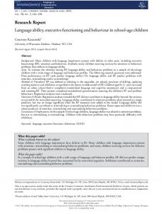
Starting with a description of the algorithm in ImageCL, our source-to-source compiler generates multiple candidate implementations in OpenCL, each with a different set of optimizations applied. The auto-tuner then picks the best implementation for a given device. One can thus easily generate multiple, high-performing versions for different devices from a single source, achieving greater performance portability. This is illustrated in Figure 1 A more detailed view of how the source-to-source compiler works together with the auto-tuner to find the best implementation for a given device can be found in Figure 2. Initially, the ImageCL code is analyzed to find the potential optimizations, that is, the tuning parameters and their possible values. Next, the auto-tuner explores the parameter space by selecting specific values for the tuning parameters, generating the corresponding OpenCL code with the source-to-source compiler, compiling it with the device compiler, and executing and timing it on the relevant device. The procedure is repeated using some arbitrary search method until the auto-tuner arrives at what it believes to be the best parameter values. Finally, the source-to-source compiler uses these parameter values to generate the final implementation. An analytical performance model or expert programmer knowledge could be used to determine parameter values directly. However, we believe the complexity and rapid development of the hardware makes auto-tuning a more robust option and therefore intend our source-to-source compiler to be used with an auto-tuner. While any general purpose auto-tuning framework can be used, our compiler was designed with the auto-tuner of our previous work1,2 in mind.
FIGURE 1
Overview of how the ImageCL source-to-source compiler would work with an auto-tuner
FIGURE 2
Detailed view of source-to-source compiler—auto-tuner interface
6 of 22
FALCH AND ELSTER
Our auto-tuner uses a machine learning-based performance model to find promising parameter configurations, to speed up the search. In particular, the auto-tuner will execute the code of several randomly selected parameter configurations and record the execution times. These data are then used to build an artificial neural network performance model, which can predict the execution time of unseen configurations. The model is then used to predict the execution time of all possible configurations, which can be done, even for large search spaces, since model evaluation is cheap. In a second step, some of the configurations with the best predicted execution times are executed, and the configuration with the best actual execution time of these is returned by the auto-tuner. We generate OpenCL since it is supported by multiple vendors and targets a broad range of devices. Compared to generating device-specific assembly, it reduces the engineering effort and allows us to leverage optimizations performed by the device OpenCL compilers.
5
THE IMAGECL LANGUAGE
The ImageCL programming language is designed to make it easy to write image processing kernels for heterogeneous hardware and be used together with the FAST framework. An example of the language is shown in Listing 1,‡ which implements a simple 3 × 3 box filter for blurring. While having features specifically designed for image processing, it can also be viewed as a simplified form of OpenCL instead of an image processing DSL. With the exception of some restrictions outlined below, ImageCL programs can contain arbitrary code with a syntax identical to OpenCL C. It can therefore be used to write general purpose programs, and can work in a standalone fashion without FAST.
ImageCL is based on the same programming models as OpenCL, where a kernel is executed in parallel by many threads, but makes the following changes: • Simplifications: – Single-level thread hierarchy. – Single memory space. • Image processing features: – Image data type with: * Parameterized pixel type. * 2D indexing. * Boundary conditions. – Pragmas to specify: * Thread defining grid. * Boundary conditions. * Force optimizations on/off. * Indicate maximum size of arrays (needed for some optimizations). In the following, we will describe these changes in more detail, starting with the simplifications. Firstly, in OpenCL, the programmer specifies a two-level thread hierarchy. This concept is abstracted away in ImageCL and replaced with a flat thread space. In particular, the user specifies an Image (described below), and a grid of logical threads, with the same size and dimensionality as the Image is created. The kernel is the work performed by one such logical thread, and it is intended to work on its corresponding pixel, although this is not a requirement. The built-in variables
‡ Further examples can be found along with the source code for the compiler at https://github.com/acelster/ImageCL.
7 of 22
FALCH AND ELSTER
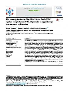
(A) Clamped: values outside are (B) Constant: values outside the set to that of the closest pixel image are set to some constant, inside the image. e.g. 0. FIGURE 3
Different boundary conditions
idx and idy store the index of the thread and can be used to index the thread grid defining Image to find the pixel of the thread. If Images are not used, the size of the logical thread grid can be specified manually. Secondly, OpenCL has a complex memory hierarchy, with multiple different logical memory spaces. These are typically mapped to different hardware memory spaces with different performance characteristics, as described in Section 2. This memory hierarchy is also abstracted away in ImageCL, and the programmer only deals with a single flat address space. In addition, ImageCL includes the Image data type, which is intended to store an image, supports 2D indexing, as shown in Listing 1, and can be templated with the pixel type. One can also specify different boundary conditions, making it possible to read outside an Image with well-defined results, a situation which frequently arises in stencil algorithms. We currently support constant and clamped boundary conditions, illustrated in Figure 3. Image comes in addition to, and does not replace, the data types supported by OpenCL, such as regular arrays. The ImageCL language also includes a small number of compiler directives. The most important is the already described grid directive, which can be used to determine which Image to base the thread grid on, as shown in Listing 1, or the size of the grid directly when no Images are used. Other directives specify boundary conditions, upper bounds on sizes of arrays, needed for some optimizations, or are used to force optimizations on or off. The present features of ImageCL are rich enough to express a wide range of parallel image processing as well as general purpose algorithms. However, some features, required for more complex algorithms, are lacking. There are currently • No work-group barriers/synchronization (because there are no work-groups). • No recursion. Since work-groups (as well as local memory) have been deliberately abstracted away, there are no work-group synchronization (e.g. barrier() [global barriers can still be achieved by returning control to the host]). We are working on addressing this issue by adding communication primitives (like reductions) as well as making it possible to optionally control the work-groups. Furthermore, due to limitations of the current implementation of the data flow analysis, the kernel must be written as a single function.
5.1
Implementation
Our ImageCL source-to-source compiler is implemented using the ROSE50 compiler framework. Before being given to the compiler proper, a few typedefs and declarations are added to the source code (e.g. declaring idx and idy, declaring an Image class), necessary to make it valid C++, which ROSE can handle directly. ROSE can generate OpenCL. Our compiler can either analyze the input code to find possible tuning parameters, or read values for the tuning parameters, and apply the relevant transformations to generate OpenCL. The analysis examines the structure of the abstract syntax tree (AST) and performs various data-flow analyses. The transformations are applied by modifying the AST. Since the ImageCL programming model is so close to that of OpenCL, generating naive, unoptimized OpenCL, is straightforward. It involves replacing idx and idy with thread index calculations, converting Images to 1D arrays as well as updating their index calculations, and adding code to implement the boundary conditions. Finally, OpenCL keywords like __kernel and __global must be added. In addition to the kernel code itself, we also generate host code to launch the kernel. We can either generate host code which can be used as a filter in FAST, or as a standalone function, callable from any C/C++ application.
5.2
Tuning parameters
Our tuning parameters are summarized in Table 1 and will be described further in this section.
8 of 22
FALCH AND ELSTER
TABLE 1
Tuning parameters
Parameter
Description
Work-group size
The size of a work-group in each dimension.
Thread coarsening
The number of logical threads processed by each real thread in each dimension.
Image memory
Whether or not to use image memory. One parameter for each applicable array.
Constant memory
Whether or not to use constant memory. One parameter for each applicable array.
Local memory
Whether or not to use local memory. One parameter for each applicable array.
Thread mapping
To use blocking or interleaved thread mapping.
Loop unrolling
Loop unroll factor for each applicable loop.
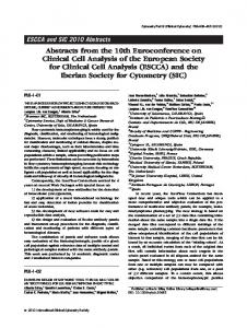
(A) Blocking FIGURE 4
(B) Interleaved
(C) Interleaved in work-group
Thread mappings. Cells correspond to logical threads, colors to real threads, and pattern to different work-groups
Some of the optimizations, in particular, the local memory optimization, are motivated by computational patterns frequently occurring in image processing, in particular stencil computations. They will therefore be most applicable and have the largest impact, for such applications. Furthermore, optimizations involving the OpenCL memory hierarchy may have little or no effect on CPUs, where this hierarchy is placed entirely in main memory. A capable auto-tuner will be able to handle such effectless parameters.
5.2.1
Work-group size
As described above, ImageCL has a flat thread space, which must be mapped to the two-level thread hierarchy in OpenCL. The size and shape of the work-groups can have significant impact on performance1,2 and are therefore added as tuning parameters.
5.2.2
Thread coarsening
ImageCL has one logical thread for each pixel of the thread grid defining Image. While good performance on GPUs requires thousands of threads to keep the device busy, using one thread per pixel can lead to millions of threads, many more than required. It may therefore be beneficial to perform thread coarsening,51 that is, let each thread perform more work, while reducing the total number of threads. In ImageCL, logical threads can be merged so that each real thread (that is, each OpenCL work-item) processes a block of pixels. The sizes of this block in each dimension then become the tuning parameters. Not only the amount of work but also the shape of the block matters, as it can affect the memory access pattern. Presently, thread coarsening is implemented by wrapping the kernel in for-loops, thus executing it multiple times.
5.2.3
Thread mapping
When a single real thread (i.e., OpenCL work-item) is used to process multiple logical threads, as described above, there are several ways to distribute the logical threads, which can affect performance. Since the logical threads are organized in an n-dimensional grid, a contiguous block of logical threads can be assigned to each real thread, as illustrated in Figure 4A. While this might give good memory locality, it may results in poor coalescing. Memory transactions made by different threads on GPUs can be merged, or coalesced, into fewer transactions if the accesses are close together. It might therefore be better to interleave the logical threads, as shown in Figure 4B. Thus, if the real threads access the pixels of their logical threads sequentially, they will access a contiguous block of pixels, leading to coalesced loads. Because of this potential performance impact, we add whether to use blocked or interleaved thread assignment as a tuning parameter. The implementation of this parameter simply requires different indexing calculations. When the local memory optimization described below is used, the interleaving is performed within each work-group, as illustrated in Figure 4C.
5.2.4
Memory spaces
In ImageCL, there is only a single address space, by default mapped to OpenCL global memory. However, using other OpenCL memory spaces can often affect performance, as described in Section 2, and is therefore included as tuning parameters. The data under consideration are either Images, or general arrays. In the following, we will refer to both as arrays, unless the distinction is necessary. Image and Constant Memory have restrictions on how they can be accessed. To determine if an array can be placed in either of them, we therefore check if it is only accessed in a read-only or write-only manner (image memory) or only read-only (constant memory). Since we disallow aliasing, this is done by checking every access to the array. For constant memory we also make sure the array is sufficiently small. Implementing these tuning parameters is straightforward and involves changing the array declaration and/or access.
FALCH AND ELSTER
9 of 22
Local Memory can be used if an Image is only read from and each thread reads from a fixed size neighborhood, or stencil, around its pixel, the size of which can be determined at compile time. In such a case, the areas read by neighboring threads will overlap, and loading the data once into local memory, and accessing it there multiple times may therefore be beneficial. To determine the size of the stencil, that is, the area around its central pixel a thread reads from, we find all the relevant Image references, and make sure they have the form image[idx + c1][idy + c2]. We then use constant propagation to determine the values of c1 and c2. Often, c1 and c2 are not constants, but depend on the iteration variable of for-loops with a fixed range, as in Listing 1. In such cases, we use a modified version of constant propagation where we allow each variable to take on a small set of constant values. If the values of c1 or c2 cannot be determined at compile time, the analysis fails, and local memory is not used. If the local memory optimization is applied, each work-group initially cooperatively loads the part of the array it will access into local memory. Loads from global memory are then replaced with loads from local memory. In general, parts of the stencil might fall outside the Image being read from, and it might also be the case that the Image read from is smaller than the thread grid. Since we restrict this transformation to Images, their boundary conditions ensures that well-defined values can be returned in these cases. Since we only consider cases where idx and idy are not multiplied, divided, taken the modulo of etc., there is a well-defined mapping from the logical threads of the thread grid to the pixels of any size array, ensuring that the real threads of a work-group work on a contiguous area, which can easily be computed. The read-only requirement is needed to ensure correctness, since we presently do not have any synchronization primitives.
5.2.5
Loop unrolling
Loop unrolling involves replacing the loop body with multiple copies of itself, while adjusting the number of iterations accordingly. As this is well known to impact performance, we add the loop unrolling factor as a tuning parameter.
6
DISTRIBUTED IMAGECL
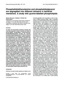
In this section, we will show how we have extended the source-to-source compiler with multi-device and multi-node support. This makes it possible to write a single ImageCL kernel, from which our compiler can generate OpenCL kernels along with orchestration code, so that the kernel can be executed on multiple devices in a node, or on the (multiple devices of) multiple nodes in a cluster. Thus, with this extension, ImageCL can seamlessly scale from a single device to an entire cluster. This is illustrated in Figure 5.
FIGURE 5 Distributed ImageCL. Input data are distributed to different devices in different nodes, where the computation is performed, before the results are gathered. For the large grid, the threads of the devices access disjoint regions, indicated by colors, and it can be scattered. For the small grid, all threads access the entire grid, and it must be broadcasted
10 of 22
FALCH AND ELSTER
The implementation of this extension is fairly straightforward and is not considered a major contribution, but instead provides us with an infrastructure for evaluating our load balancing and scalability prediction techniques, as described in Section 7. While we use ImageCL, these techniques can also be applied in other settings. ImageCL, in its current version, does not support any communication or synchronization primitives. The ImageCL and corresponding OpenCL kernels are therefore embarrassingly parallel and can easily be scaled to multiple devices, by splitting the thread space and assigning a part of it to each available device. In addition, some orchestration code is needed to split up and distribute the input data as appropriate, as well as gather and combine the results. The orchestration code is implemented using a combination of OpenMP and MPI. OpenMP is used within each node, with one thread for each device, while MPI is used between nodes, with one process per node. After having divided the thread space among the available devices, we must determine how the input and output data should be distributed and gathered. In ImageCL, it is typically the case that a thread works on a single element, or a small neighborhood, of an ImageCL Image (e.g. a pixel or its neighborhood in an image). If this is the case, we only distribute the part of the Image which is accessed by the threads running on one device, to that device. On the other hand, if it cannot be determined that the threads of a device will only access a specific region of an Image, or we deal with general arrays, the entire array is sent to every device. For output Images, on the other hand, we currently only support the case where the threads of a device writes to a specific region (disjoint from the corresponding regions of other devices) which can be determined at compile time. ImageCL already contains functionality for determining the areas of Images accessed by different threads, as described in Section 5.2.4. On a single node, the shared memory nature of OpenMP makes the process of distributing and gathering the inputs and outputs straightforward. For the distributed case, MPIs broadcast, scatter and gather functions are used. The internal boundaries of Images present some additional challenges. For many applications, like stencil applications, each thread will access a neighborhood around its central data point. In such cases, we must distribute overlapping regions to the different devices, that is, the region of each device gets padded with a layer of “ghost” cells. Furthermore, ImageCL can implement different global boundary conditions for Images, where threads along the global boundary of the array executes special code. When multiple devices are used, the threads along the boundaries might be part of the global border, or an internal border. We must therefore also distribute information to each device about what region of the global Image it is processing, so that it can handle this appropriately.
7
PERFORMANCE MODELING
The goal of our performance model is to predict the performance of new, unseen, applications as a function of the problem size, on different devices. We restrict our performance modeling to regularapp lications, like stencil applications. For such applications, the execution time typically scales linearly with the problem size, that is, the throughput, measured in input data points (e.g. pixels) per time, is constant. To predict the execution time for a given application on a single device, one could therefore run it on a small input, measure the throughput, and extrapolate to the desired problem size. The throughput will, however, typically vary on different devices. This is because the nature of the work performed by the application will be more or less suited to different kinds of architectures. For instance, a memory bound application will have a higher throughput on a device with higher memory bandwidth, and a application with a lot of double precision computation will have higher throughput on a device with good support for this. Thus, to predict the performance on multiple different devices, one would need to execute the relevant application on all of them to measure the throughput. Our method avoids this by executing the application on a small input on a single device and measuring performance counters. Hardware performance counters are special registers which count hardware events, such as the number of different kinds of instructions, branch mispredictions, or cache misses. The performance counter values measured during the execution of an application can therefore capture and describe the nature of the computations performed. For this reason, they can be used as a sort of application profile, from which it is possible to predict the throughput on multiple different devices, without ever executing the application on all of them. We do this prediction using machine learning. In an offline phase we collect training data, which we use to build a model that later can be used to predict throughput. In particular, we take a large number of benchmarks and run them with small inputs on one device, where we record the performance counter values. We then run the same training applications on multiple other devices and measure the throughput. We then give all these data to a machine learning algorithm, which builds one performance model for each device. Later, we can predict the throughput of a new, unseen application on multiple different devices, by collecting the performance counters on one device and using one or more such models. An overview of our approach can be found in Figure 6. While gathering the training data, and training the models can take some time, this is a one time cost for a given class of applications and set of devices. Our method has low overhead at runtime, since performance counter measurements can be done cheaply. Furthermore, it does in principle not require access to source code, but can be used on unmodified binaries. While several different kinds of devices support performance counters, we measure performance counters on the CPU, as we found this to be faster and more flexible than doing it, e.g., on the GPU. As will be described in further detail below, we use ImageCL to generate our benchmarks. This allows us to generate both C and OpenCL versions of the same benchmarks. For simplicity, we measure the performance counters when executing the C version of the code, while predicting the throughput of the OpenCL version on different devices. We used the PAPI API52 on an Intel i7 3770K for performance counter measurements. This gave us access to 44 different performance counters. Of these, 28 are related to cache misses (for various levels of instruction and data caches), 7 are related to branching and branch prediction, 4 to
FALCH AND ELSTER
FIGURE 6
11 of 22
Overview of performance modeling method
floating point operations, 2 to TLB misses, and 3 to cycle and instruction counts. Using a different tool or a different CPU can result in a different set of counters. As described in Section 2, a large number of different machine learning algorithms exist, but few well-founded guidelines on which to use for different situations. We therefore experimented extensively with different algorithms, before we found that AdaBoosted regression trees gave the best performance of the methods we evaluated. However, further experimentation, including a more thorough search of the parameter space of the different algorithms, could potentially reveal even better methods.
7.1
Synthetic benchmarks
Machine learning methods, like our approach, can require a significant amount of training data. For this reason, we used synthetic benchmarks, which we could easily generate as many of as needed. Furthermore, it gave us the ability to control the computations performed by the benchmarks, so that they matched, and therefore could be sufficiently described by, the available performance counters. The benchmarks are all 2D stencil computations, which read from a stencil of a 2D array, perform computations with these values, and finally write back a single value to a different 2D array. To create different benchmarks, we varied the computation as well as memory access pattern, covering the space of possible implementations. In particular, we varied the following aspects of the benchmarks: • The size and shape of the stencil. • The amount of computation relative to memory accesses. • The ratio of single to double precision floating point operations. • The ratio of divisions to other arithmetic operations. • The ratio of unpredictable to predictable branches. Thus, although the benchmarks are synthetic, they represent, and can be used as realistic proxies for, a broad class of stencil applications. We implemented our benchmark generator as a Python script, which generated ImageCL output. We then used our ImageCL compiler to generate OpenCL kernels and orchestration code for a single device, as well as multiple devices in a node, or multiple nodes, in addition to the C code used to measure the performance counters. The generated orchestration code allowed us to control the amount of work assigned to each device, enabling the experiments outlined below.
7.2
Single node load balancing
In the previous section, we described our performance modeling scheme. One use case for this scheme is to divide the work of a new, unseen, kernel between multiple different devices in the same node. This would be done by executing the kernel on a small input on one device, and recording
12 of 22
FALCH AND ELSTER
performance counters. The counter values would then be fed to multiple, previously trained models, to predict the throughput on each of the available devices. The devices would then be given a share of the work based on their throughput, so that the faster devices would be given more work, making them all finish at the same time. If needed, it is also possible to incorporate host-to-device transfer times. The bandwidth is generally independent of the application and can be measured once for each device. Thus, if the throughput on device i is Ti , the bandwidth is Bi , and the fraction of the work ri , the (normalized) execution time becomes ( t i = ri
2 1 + Ti Bi
)
The execution time for all the devices is minimized when the work is divided so that all of the devices finish at the same time. If we have n devices, we can therefore find the amount of work for each device by solving the n equations: ti = ti+1 ∀i ∈ 1, 2, … , n − 1 n ∑ ri = 1 i=1
Where the first n − 1 equations ensures that the execution times are equal, and the last that the normalized amount of work sums to 1.
7.3
Multinode scaling prediction
Another potential use of our performance modeling scheme is to determine the number of nodes to use in a heterogeneous cluster. In general, the total execution time for an application on a cluster will be the sum of the computation time and the communication time (minus any overlap), where both can be application dependent. While the computation time (on each node) will generally decrease as the number of nodes are increased, the communication time, as well as other overhead, may increase. It might therefore be ideal to use fewer than all available nodes. In the following, we will simplify the analysis by restricting ourselves to ImaceCL-like applications, as described in Section 6. These applications follow the bulk synchronous parallel (BSP) model,32,53 consisting of stages of parallel computation on local data, interleaved with global communication and synchronization. Our method is, however, not tied to ImageCL and can also be generalized to other models than BSP. For BSP-like applications, the total execution time on a cluster can be modeled as m
j Tcluster = Tscatter + maxTcomp + Tgather j=0
j where Tscatter and Tgather are the time required to distribute the input and gather the results, respectively, and Tcomp is the computation time on node j.
That is, the total execution time is the sum of the time for scattering and gathering the data, and the computation time on the slowest node. Clearly, we should ensure that Tcomp is equal on all the nodes to minimize this expression. To find the best number of nodes to use, we use our performance modeling method to predict the throughput on all the devices of the cluster, as described previously. Then, the amount of work for each device can be determined with the same calculation used for a single node, described in the previous subsection, but modified to include all the devices of the cluster. The amount of work for each node is then the sum of the work of its devices. This naturally handles the situation where each node consists of different devices. Furthermore, none of the devices of the compute nodes have to be available on the root node, where the performance prediction is taking place. Next, since Tscatter and Tgather are largely application independent, they can be measured for different problem sizes and number of nodes for a single application. These data can then be used to train a predictive model. Finally, given a new application and input size, we can use the computation and communication models to predict the execution time using from 1 node to all the available nodes, and then pick the number of nodes with the minimum predicted execution time.
8
RESULTS
In this section we will present the results of an evaluation of our approach. We will first consider generating and auto-tuning ImageCL code for a single device. Next, we will consider load balancing for the multi-device extension to ImageCL. We will first look at the accuracy of the performance models in isolation, before evaluating their ability to balance load in a single node, and finally their ability to pick the best number of nodes in a cluster. For the single device case, the benchmarks we use will be described further in that section. For the multi-device case, we will use the benchmarks described in Section 7.1, as well as the multi-device extension to ImageCL as an infrastructure to distribute the work.
8.1
Single device
To evaluate ImageCL we implemented three image processing benchmarks and compared performance with other state-of-the-art solutions. To evaluate performance portability, we tested on a range of different hardware devices.
13 of 22
FALCH AND ELSTER
TABLE 2
Device specifications Nvidia GTX 960
Nvidia K40
AMD 7970
Intel i7 4771
Memory bandwidth (GB/s)
112
288
264
25.6
TFlop/s
2.3
4.29
3.79
0.45
The benchmarks used were separable convolution, non-separable convolution, and Harris corner detection. Convolution was chosen because it is extensively used in image processing, e.g., for the ubiquitous Gaussian blurring. It also serves as a proxy for other stencil computations. Harris corner detection was chosen as an example of a more complex algorithm. For evaluation, we used three different GPUs, an Nvidia GeForce GTX 960, an Nvidia Tesla K40, and an AMD Radeon HD 7970, as well as a Intel i7 4771 CPU. Some pertinent details of the hardware can be found in Table 2. We compared our performance against Halide,17 HIPACC,18 and OpenCV.54 Halide and HIPACC, described in Section 2, are domain-specific languages for image processing and can generate high-performance CPU and GPU implementations. OpenCV is a widely used library for image processing. It is highly optimized and contains implementations for both CPUs and GPUs. We used OpenCV 3.0, the 2015/10/22 release of Halide and HIPACC 0.8.1. HIPACC allows the target device and architecture to be specified, so that appropriate optimizations can be applied. The version of HIPACC we used does not support the AMD 7970. We therefore used the latest generation of AMD devices it supports instead. While Halide claims that its code can be auto-tuned, no auto-tuner or auto-tuning interface is distributed with the source code. We therefore performed extensive manual tuning. As described in Section 3, Halide code is divided into a functional description of the algorithm, and a schedule, describing parallelization, tiling, vectorization, etc. The manual tuning was therefore carried out by systematically trying out different possible Halide schedules for each device/benchmark combination. The ImageCL implementations were auto-tuned with the machine learning-based auto-tuner from our previous work,1,2 which is described in Section 4. Both HIPACC and Halide can generate either OpenCL or CUDA when targeting Nvidia devices. For HIPACC, we used the CUDA version, and for Halide the OpenCL version, since these performed best. Similarly, HIPACC can generate OpenCL and C++ code for the CPU. Since the OpenCL versions performed better, we report those results. Both Halide and HIPACC can generate specialised code if the values of the filters are known at code generation time. We evaluated both options, for the separable convolution, the filter values are known at code generation time, while they are only known at run time for the non-separable convolution. The execution times reported does not include CPU-GPU memory transfers, preparing inputs, etc., as this will be the same for all alternatives. Due to time constraints, we only compared against OpenCV for the Harris corner detection. Figure 7 shows the results. For separable convolution, we used a 4096×4096 image with pixels of type float, a 5×5 filter, and a constant boundary condition. ImageCL was faster than the alternatives on the GPUs, achieving speedups between 1.06 and 2.25, with the sole exception of Halide on the GTX 960, which was 9.1% faster than ImageCL. On the CPU, ImageCL was 1.05 and 1.11 times slower than Halide and OpenCV, but was 1.23 times faster than HIPACC. For non-separable convolution, we used a 8192×8192 image with pixels of type unsigned char, a 5×5 filter, and a clamped boundary condition. ImageCL was faster than the alternatives on the GPUs, achieving speedups between 1.17 and 2.82, with the sole exception of OpenCV on the AMD 7970, which was 43.4% faster than ImageCL. On the CPU, ImageCL performed worst, only 1.06 times slower than OpenCV, but 4.24 times slower than Halide. For Harris corner detection, we used a 5120×5120 image with pixels of type float, and a block size of 2×2. ImageCL significantly outperformed OpenCV on the AMD 7970, K40, and Intel i7, achieving speedups of 3.15, 2.11, and 4.57 respectively. On the GTX 960, the performance was more similar, with ImageCL achieving a speedup of 1.08. In all cases, the GPUs outperform the CPU. This is caused by the significantly higher memory bandwidth of the GPUs, as shown in Table 2. For this reason, it is interesting to look at how close the results are to the theoretical peak performance of each device. Since stencil benchmarks are memory bound, we can do this by comparing the achieved bandwidth with the maximum bandwidth of the devices. If we, to get at theoretical lower bound, assume perfect caching, we only need to read the entire image once, and write it once. The achieved bandwidth then becomes two times the size of the image, divided by the execution time. In Figure 8 we show the achieved bandwidth, as a percentage of the theoretical peak bandwidth, for separable convolution. The relative performance of the different languages/frameworks is the same as in Figure 7A. ImageCL achieves between 30% and 40% of peak for the GPUs, and around 20% for the CPU. This might indicate that support for CPU-specific features, notably vectorization, might need to be improved. While the percentage of peak is relatively low in all cases, it should be kept in mind that the peak is a theoretical minimum, based on the assumption of perfect caching, and is not attainable in practice. ImageCL performs comparatively well in the single device case because it is able to apply a wide range of optimizations and use auto-tuning to pick the correct optimizations for a given device and benchmark. For example, the good performance compared to Halide on the K40 is caused in part by ImageCL using image memory, an optimization Halide does not expose and therefore cannot be applied even if the programmer suspects it might help. The varying and sometimes poor performance of OpenCV illustrates the problem of performance portability. It has separate implementations
14 of 22
FALCH AND ELSTER
(A) Separable convolution
(B) Non-separable convolution
(C) Harris corner detection FIGURE 7
Execution times on different hardware with different benchmarks
FIGURE 8
Percentage of peak bandwidth
for the CPU and GPUs, a solution that requires extra work and scales poorly. For the GPUs, it is increasingly difficult to write a single implementation that performs well on all of them. ImageCL's use of auto-tuning represents a more robust and scalable solution. However, some optimizations cannot be applied in the current version of ImageCL. Halide achieves good performance, in particular on the GTX 690 by merging the two separable convolution kernels, caching the intermediary result in local memory. Due to the lack of synchronization and communication primitives, this optimization can currently not be applied in ImageCL. We suspect that the poor results for non-separable convolution on the CPU is caused by lack of vectorization. Our compiler does currently not perform vectorization, instead relying on the vectorization capabilities of the OpenCL runtime, which performed better for the separable convolution and corner detection, than the non-separable convolution. The poor performance for non-separable convolution on the CPU is also caused by the implementation of the clamped boundary condition. If the constant boundary condition is used, the execution time is reduced by a factor of 2. As such, it is not a fundamental flaw of our approach, and using auto-tuning to pick different implementations of the boundary condition for different devices could overcome this issue. Despite good results, the time required for auto-tuning, even using our machine learning-based auto-tuner, 1,2 can be a significant drawback. For the cases presented, the auto-tuner executed around 1700 valid candidate implementations during its search for each device/benchmark
15 of 22
FALCH AND ELSTER
Configurations found by auto-tuner for the row (R) and column (C) kernels of the separable convolution
TABLE 3
Device
AMD 7970 GTX 960
K40
Intel i7
Kernel
R
C
R
C
R
C
R
C
Px./thread X
4
2
1
1
2
2
128
32
Px./thread Y
1
2
1
2
1
2
1
1
Work-group X
64
16
16
64
16
16
8
16
Work-group Y
4
16
16
4
16
16
1
2
Interleaved
1
1
0
0
0
0
1
1
Image mem.
0
1
1
0
1
1
0
0
Local mem.
1
1
0
0
0
0
0
0
Constant mem.
1
1
1
1
1
1
1
1
Unroll loop 1
0
1
0
0
1
0
1
0
TABLE 4 Configurations found by auto-tuner for the non-separable convolution
Device
AMD 7970
GTX 960
K40
Intel i7
Px/thread X
4
4
4
256
Px/thread Y
16
4
8
2
Work-group X
64
8
32
2
Work-group Y
4
32
4
8
Interleaved
0
1
0
1
Image mem
0
0
1
0
Local mem
0
1
0
0
Constant mem
1
1
1
1
Unroll loop 1
1
1
1
1
Unroll loop 2
0
1
1
1
TABLE 5 Configurations found by auto-tuner for the Sobel kernel of the Harris corner detection
Device
AMD 7970
GTX 960
K40
Intel i7
Px/thread X
1
4
1
32
Px/thread Y
1
2
4
4
Work-group X
128
32
32
64
Work-group Y
1
2
4
1
Interleaved
0
1
0
0
Image mem
0
0
1
0
Local mem
0
1
0
0
combination. This required around 2 hours in total. For each candidate implementation, running the actual kernel takes milliseconds, additional time is required to prepare inputs and transfer data to and from the GPU. More significantly, each candidate implementation must be compiled by our compiler and the OpenCL compiler which can take up to 1-3 seconds. In comparison, OpenCV and HIPACC have no tuning overhead, while the manual tuning for Halide required several hours. Because of the overhead, this kind of auto-tuning will be most useful for code that is executed many times, like library functions. The good results achieved here, as well as in our previous work1,2 gives us some confidence in our auto-tuners abilities, but it does not give any guarantees about how close the solution found is to the globally best one, which can only be found by time-consuming exhaustive search. Auto-tuning might be more challenging for larger applications with more complex search spaces. Table 3 shows the parameters, and the values found, by the auto-tuner for separable convolution. Tables 4, 5, and 6 show the same data for the non-separable convolution, and the Sobel and Harris kernels of the Harris corner detection, respectively.
8.2
Accuracy of the performance model
Figure 9 shows the accuracy of the performance model we developed for load balancing, for different CPU and GPU devices, as we vary the amount of training data. We drew the training samples randomly from a pool of 3000 benchmarks, generated as described in Section 7.1, and measured the predictive accuracy using 200 separate benchmarks (i.e. not a subset of those used for training). Since the performance of the model depends on
16 of 22
FALCH AND ELSTER
TABLE 6 Configurations found by auto-tuner for the Harris kernel of the Harris corner detection
FIGURE 9
Device
AMD 7970
GTX 960
K40
Intel i7
Px/thread X
1
1
32
8
Px/thread Y
1
2
2
2
Work-group X
32
128
64
32
Work-group Y
8
2
16
2
Interleaved
0
0
1
0
Image mem dx
1
1
1
0
Image mem dy
1
1
1
0
Local mem dx
1
1
0
0
Local mem dy
1
1
0
0
Loop 1
1
0
0
1
Loop 2
0
1
0
0
Predictive accuracy as training data are increased
which benchmarks were used for training we report the average of 10 runs. The metric we use is mean relative error, that is, the mean (across all the benchmarks used for evaluation) of the (absolute value of the) relative error when comparing the predicted throughput to the actual throughput. As we can see, the accuracy improves as more training data are used, but levels off after about 500 training benchmarks. We also note that the accuracy differs significantly between devices, for 1000 training benchmarks, the mean relative error for the Nvidia GTX 980 is 8.3%, while it is only 2.4% for the AMD Radeon 7970. The results shown in Figure 10 demonstrate the need for multiple performance counters, by comparing it to two simpler approaches, using just CPU time or CPU instructions. For these two simpler approaches, we train a machine learning model to predict the device throughput using just the measured CPU execution time, or just the number of CPU instructions, rather than the full set of performance counters, when executing a small problem set on the CPU. Here, we use 1000 benchmarks for training and report the average of 10 runs. As we can see, if we use just CPU time or CPU instructions, the resulting accuracy is significantly worse than if all the counters are used. This is especially pronounced on the GTX 980 and GTX 780, where using just CPU time or instructions give mean relative errors between 60% and 102%, for the other devices the corresponding numbers are 15% and 30%. When all counters are used, the mean relative error is less than 10% for all devices. It might seem counterintuitive that we cannot predict the CPU throughput perfectly using just the CPU time. However, keep in mind that we are trying to predict the throughput of the full problem set executed with OpenCL, based on the throughput of a small input using C. The ability of the OpenCL compiler to parallelize and optimize the code depends on the executions performed, and the OpenCL throughput is therefore not proportional to the C throughput. If we had used OpenCL when measuring the performance counters, the situation would be different. The great difference in accuracy of the performance model we see between the different devices can be explained by considering the variation in throughput of the benchmarks, and how well this variation can be explained by the available performance counters. If we compare the GTX 760 and GTX 980 on one hand with the K40 on the other, the better accuracy achieved for the latter can in part be explained by the fact the throughput varies less on this device, making it easier to build a predictive model. This is consistent with the results in Figure 10, which shows how the accuracy when using just CPU time or instructions is particularly bad for the GTX devices, due to the large variance in their execution times. Furthermore, while the variance matters, the degree to which the performance counters can explain this variance is also important. For instance, the variance is larger for the AMD GPU than the K40, but the accuracy is better, because the throughput depends heavily on the ratio of double precision to single
FALCH AND ELSTER
FIGURE 10
Accuracy when all performance counters are used for prediction, compared to using just CPU time or CPU instructions
FIGURE 11
Boxplot, showing distribution of ratio of slowest to fastest execution time
17 of 22
precision computation, which can be measured directly. On the other hand, we theorize that the memory access pattern have a larger impact on the K40. Since we can only measure the nature of the memory access pattern indirectly (e.g. using cache misses), the predictive accuracy is worse.
8.3
Load balance
In this section we will look at how well we are able to balance the load of a single kernel between different devices in a single node, based on the predicted throughput, as described in Section 7.2. We evaluated this by using nodes with multiple devices. For each node, we took 100 benchmarks, and divided the load between the devices in the node based on performance models trained using 1000 separate benchmarks (i.e. the benchmarks used for evaluation were not a subset of those used for training). The benchmarks were generated as described in Section 7.1. For our experiments, we used two different nodes, one consisting of an Intel i7 3770 CPU and an Nvidia GTX 980 GPU, while the other combined Nvidia GTX 760 and K40 GPUs. On the second node, the CPU was not used. We compared our method to a simpler, fixed scheme, that is, a load balancing scheme which assigns a fixed ratio of the work to the different devices in the same way for every benchmark. Such a scheme can work well if all the benchmarks are similar, but may perform poorly for diverse benchmarks, since their throughput on the different devices will vary. The fixed work ratios were the best found using exhaustive search (with 1% granularity) based on recorded execution times. Figure 11 shows the imbalance distribution for the 100 benchmarks. When work is divided between multiple devices, we get one execution time for each device. We calculated the imbalance by dividing the longest of these by the shortest. Ideally, with perfect load balancing, the execution times are equal, and this value will be 1. With poor load balancing, too much work will be assigned to one device, making the execution times more different, and the ratio of the longest to the shortest execution time will be higher. We achieve good results, with mean values between 1.07 and 1.08, and a standard deviation between 0.09 and 0.11. There are however a few outliers, where the imbalance is up to 1.65. We also see the limitations of the static scheme, which where the mean imbalances are between 1.53 and 2.15.
18 of 22
FALCH AND ELSTER
Another way to measure the quality of the load balancing scheme is to look at the total slowdown of all the benchmarks, compared to an oracle, which is able to perfectly divide the load. We compute this by taking the sum of the execution times of all the benchmarks. If the load is unevenly balanced, the execution time will be longer, and we get a slowdown compared to the oracle. The oracle results were created by measuring the throughputs of the benchmarks directly on each device, and using this as the basis for dividing the load, rather than the predicted throughputs. We also compare with the naive, fixed approach described above. Figure 12 shows the results. As we can see, our scheme achieves good results, with slowdowns between 1.03 and 1.04. The fixed scheme, on the other hand, gets slowdowns between 1.11 and 1.22, because it is unable to adapt to the variation in the different benchmarks.
8.4
Multinode scalability prediction
In this section, we look at how well our performance modeling scheme is able to pick the correct number of nodes to use in a cluster. We evaluated this by running 100 benchmarks, generated as described in Section 7.1, and for each benchmark, use the method described in Section 7.3 to determine the number of nodes to use. We then calculated the slowdown of this approach compared to that of an oracle, which would always know the best number of nodes to use. We also compared against two naive techniques, always using just one node, and always using all available nodes. The oracle was developed by simply trying all possible numbers of nodes, and picking the best one, for each benchmark. We used two different clusters, clrocks, consisting of 7 off-the-shelf desktop computers as nodes, each equipped with an Nvidia GTX 480 card, connected with Gigabit Ethernet, and numascale, a Numascale cluster consisting of 5 nodes, each with a Nvidia GTX 980 card, and a custom interconnect, whith a theoretical bandwith of 19.2 GB/s per link.55,56 Given the relatively small size of the clusters used for evaluation, we deliberately generated benchmarks with poor scaling behavior, so that the best number of nodes to use would be between 1 and all the nodes. The poor scalability was primarily achieved by increasing the stencil size (and thus, the amount of communication). The results are shown in Figure 13. As we can see, our scheme achieves performance close to that of the oracle with slowdowns of 1.02 in both cases. We significantly outperform the naive schemes, where the slowdowns are between 1.11 and 1.27.
FIGURE 12
Slowdown compared to perfect load balancing
FIGURE 13
Slowdown compared to using best number of nodes
FALCH AND ELSTER
9
19 of 22
DISCUSSION
The intuitive idea behind our performance modeling method is that measured performance counters can be used to describe an application (i.e. the number and type of floating point calculations, the number of memory accesses), and that this description can be used to predict performance on a different device (where, i.e., the relative performance of floating point and memory accesses might be different). While performance counters can give detailed information about the nature of an application, they do not give a complete view, which may cause predictions made based on them to be less accurate. This can be caused by two different problems. Firstly, there might not be a relevant counter on the measuring device. For instance, there might not be a counter to distinguish between add and multiply operations on the measuring device, when the relative rates of these have great impact on performance on the target device. Secondly, there might be some factors greatly affecting performance on the target device, which does not exist or have any counterpart on the measuring device, due to architectural differences. As an example, branch divergence can impact performance on GPUs, but cannot be measured on CPUs with performance counters, not because the counter is missing, but because the event never occurs. Similarly, if counters measured during a serial run are used to measure parallel performance for general applications, there will be no way to account for, e.g., synchronization. Both these effects can to a certain degree be mitigated by using several other counters. For instance, the number of cache misses on a CPU might indirectly capture the memory access pattern, which is important on GPUs. As the preceding paragraph should make clear, the applicability of our method depends heavily on the devices used and their relative architectural differences, the counters available, and the benchmarks used. In this work we used synthetic benchmarks to train the performance model used for load balancing. This allowed us to achieve good results, because we could tailor the benchmarks to the performance counters available on the particular CPU we used. That is, we constructed the benchmarks in such a way that we could be sure that the variation in them to a large degree would be picked up by the available performance counters, by primarily varying things for which a corresponding counter existed. Clearly, this allows the performance counters to describe the benchmarks in a good way, making it possible to build highly accurate models. No machine learning method will work unless the features can describe the variation of the data. Having access to performance counters with sufficient richness to capture the nature of the class of applications under consideration is therefore necessary. However, while our benchmarks are synthetic, they are quite general and can serve as proxies for a broad class of real-life applications, in particular regular, highly data parallel applications. Furthermore, as mentioned in the previous paragraph, there is not a one-to-one relationship between the counters and what is varied in the benchmarks. We therefore believe our method could work well for real benchmarks in a more general setting. Finally, our method is not intrinsically tied to the particular CPU we used, or to CPUs as such. Any CPU, GPU, or other device with a reasonable set of performance counters could be used, subject to the caveats discussed above. In particular, we believe that we could have reversed our experiments and used counters measured on the GPUs to predict performance on the CPU, with reasonable accuracy. In our evaluation, we used our ImageCL compiler to generate the final OpenCL, as well as C code used for measuring the performance counters. However, our method is not tied to ImageCL, or, strictly speaking, OpenCL, but can work for any application which needs to balance load between different devices. Not even source code access is required, it is only necessary to be able to measure performance counters on one device for a small input. For the load balancing and scalability prediction, we used ImageCL primarily as an infrastructure. The underlying problems, dividing load evenly, and predicting the best number of nodes to use, are not tied to ImageCL and would arise for any language or framework using different devices or multiple nodes. The performance modeling methods are also not tied to ImageCL and can be generalized to other applications. An important assumption for the performance modeling part of this work is that the throughput of an application on a device is constant and does not depend on the problem size. This is mostly true for the benchmarks we consider, as our good results show. However, we did observe some variation, in particular for very small problem sizes, and this might be more pronounced for other devices and classes of applications. In such cases, it must be considered in the load balancing calculations. We also observed that the throughput of CPU devices was reduced when they were used together with GPUs on the same node. This difference was small and constant, making it easy to correct for in our case, but is also something which could be included in the modeling or calculations if it is found to have a larger and more varying impact.
10
CONCLUSION AND FUTURE WORK
The increasing popularity of heterogeneous computing has made performance portability, making code execute with good performance when moved between different devices, harder to achieve. Furthermore, determining the best way to partition work on heterogeneous hardware to minimize execution time can be difficult, since the suitability of the different devices to the application at hand must be taken into account. In this paper, we have introduced the ImageCL language and its source-to-source compiler. ImageCL is a simplified form of OpenCL with features for image processing and is translated to optimized OpenCL. Our source-to-source compiler can apply various optimizations to generate multiple candidate implementations. An auto-tuner can then pick the best implementation for a given device. We also propose an extension to our ImageCL source-to-source compiler, which allows single data parallel kernels to be executed on one device, multiple devices in a node, or on multiple nodes of a cluster. Our performance modeling approach can be used to predict the correct way to partition the work. It works by running an application on a small input on one device, and measuring performance counters. The counters are then fed to performance models which predicts the throughput of the application on multiple different devices, making it possible to partition work evenly. The models are built using machine learning by correlating performance counters and execution times on different devices for training benchmarks.
20 of 22
FALCH AND ELSTER
We have evaluated the performance of ImageCL with three image processing benchmarks and are able outperform state of the art solutions in several cases, achieving speedups of up to 4.57×. Our proposed solution therefore shows promise as a way to come closer to the goal of heterogeneous performance portability. For the distributed case, we evaluated our method on a range of different hardware devices. When balancing the load between devices in a single node, our method is only 3% slower, and when picking the correct number of nodes to use in a cluster only 2% slower, than an oracle, using synthetic benchmarks. Future work may include adding additional features, such as synchronization and communication primitives, and increased support for vectorization. Another possibility is to evaluate ImageCL with more diverse benchmarks, on a broader range of hardware, including CPUs and accelerators. For the distributed case, it would also be interesting to test our methodology with real benchmarks, and to see if our methodology could be used for more irregular applications as well. Finally, investigating how these methods could be used for one or more of the use cases in the CloudLightning EU project57 we are a part of is a possibility for further investigation.
ACKNOWLEDGMENTS The authors would like to thank NTNU IME and NTNU MedTech for their support of the Medical Computing & Visualization project, Nvidia's GPU Research Center program and NTNU for hardware donations to our NTNU/IDI HPC-Lab, and Drs. Malik M. Z. Khan and Erik Smistad for their helpful discussions. Parts of this work were funded by the European Union's Horizon 2020 Research and Innovation Programme through the CloudLightning project (http://www.cloudlightning.eu) under Grant Agreement Number 643946. The authors would also like to thank Dr. Keshav Pingali and ICES at the University of Texas at Austin for hosting us during the parts of the work for this article.
ORCID Thomas L. Falch
http://orcid.org/0000-0001-8498-4825
REFERENCES 1. Falch TL, Elster AC. Machine learning based auto-tuning for enhanced OpenCL performance portability. In: 2015 IEEE International Parallel and Distributed Processing Symposium Workshop (IPDPSW), Hyderabad, India; 2015:1231-1240. 2. Falch TL, Elster AC. Machine learning-based auto-tuning for enhanced performance portability of OpenCL applications. Concurr Comput Pract Exper. 2016;29. https://doi.org/10.1002/cpe.4029 3. Smistad E, Bozorgi M, Lindseth F. FAST: framework for heterogeneous medical image computing and visualization. Int J Comput Assisted Radiol Surg. 2015;10(11):1-12. https://doi.org/10.1007/s11548-015-1158-5 4. Falch TL, Elster AC. ImageCL: an image processing language for performance portability on heterogeneous systems. In: 2016 International Conference on High Performance Computing Simulation (HPCS), Innsbruk, Austria; 2016:562-569. 5. Smistad E, Falch TL, Bozorgi M, Elster AC, Lindseth F. Medical image segmentation on GPUs—a comprehensive review. Med Image Anal. 2015;20(1):1-18. 6. Alpaydin E. Introduction to Machine Learning. Cambridge, MA, USA: MIT Press; 2010. 7. Frigo M, Johnson SG. The design and implementation of FFTW3. Proc IEEE. 2005;93(2):216-231. Special issue on “Program Generation, Optimization, and Platform Adaptation”. 8. Whaley RC, Petitet A. Minimizing development and maintenance costs in supporting persistently optimized BLAS. Software Pract Exper. 2005;35(2):101-121. 9. Elster AC, Meyer JC. A super-efficient adaptable bit-reversal algorithm for multithreaded architectures. In: IEEE International Symposium on Parallel Distributed Processing, IPDPS 2009, Rome, Italy; 2009:1-8. 10. Yotov K, Li X, Ren G, et al. A comparison of empirical and model-driven optimization. SIGPLAN Not. 2003;38(5):63-76. 11. Bergstra J, Pinto N, Cox D. Machine learning for predictive auto-tuning with boosted regression trees. In: Innovative Parallel Computing (InPar), 2012, San Jose, CA, USA; 2012:1-9. 12. Zhang Y, Sinclair M, Chien AA. Improving performance portability in OpenCL programs. Supercomputing, Lecture Notes in Computer Science, vol. 7905. Leipzig, Germany: Springer Berlin Heidelberg; 2013:136-150. 13. Pennycook SJ, Hammond SD, Wright SA, Herdman JA, Miller I, Jarvis SA. An investigation of the performance portability of OpenCL. J Parallel Distrib Comput. 2013;73(11):1439-1450. 14. Nugteren C, Codreanu V. CLTune: a generic auto-tuner for OpenCL kernels. In: IEEE 9th International Symposium on Embedded Multicore/Manycore Systems-on-Chip (MCSoC-15), IEEE, Turin, Italy; 2015:195-202. 15. Van Deursen A, Klint P, Visser J. Domain-specific languages: an annotated bibliography. Sigplan Not. 2000;35(6):26-36. 16. Sujeeth AK, Brown KJ, Lee H, et al. Delite: a compiler architecture for performance-oriented embedded domain-specific languages. ACM Trans Embed Comput Syst. 2014;13(4s):134:1-134:25. 17. Ragan-Kelley J, Barnes C, Adams A, Paris S, Durand F, Amarasinghe S. Halide: a language and compiler for optimizing parallelism, locality, and recomputation in image processing pipelines. ACM SIGPLAN Not. 2013;48(6):519-530. 18. Membarth R, Reiche O, Hannig F, Teich J, Korner M, Eckert W. HIPAcc: a domain-specific language and compiler for image processing. IEEE Trans Parallel Distrib Syst. 2016;27(1):210-224. 19. Mullapudi RT, Vasista V, Bondhugula U. PolyMage: automatic optimization for image processing pipelines. In: Proceedings of the Twentieth International Conference on Architectural Support for Programming Languages and Operating Systems, ASPLOS '15. New York, NY, USA: ACM; 2015:429-443.
FALCH AND ELSTER
21 of 22
20. Ueng SZ, Lathara M, Baghsorkhi SS, Wen-mei WH. CUDA-lite: reducing GPU programming complexity. Languages and Compilers for Parallel Computing. Edmonton, AB, Canada: Springer; 2008:1-15. 21. Lin Z, Gao X, Wan H, Jiang B. GLES: a practical GPGPU optimizing compiler using data sharing and thread coarsening. Languages and Compilers for Parallel Computing. Hillsboro, OR, USA: Springer; 2014:36-50. 22. Yang Y, Zhou H. The implementation of a high performance GPGPU compiler. Int J Parallel Program. 2013;41(6):768-781. 23. Khan M, Basu P, Rudy G, Hall M, Chen C, Chame J. A script-based autotuning compiler system to generate high-performance CUDA code. ACM Trans Archit Code Optim. 2013;9(4):31:1-31:25. 24. Du P, Weber R, Luszczek P, Tomov S, Peterson G, Dongarra J. From CUDA to OpenCL: towards a performance-portable solution for multi-platform GPU programming. Parallel Comput. 2012;38(8):391-407. 25. Christen M, Schenk O, Burkhart H. Patus: a code generation and autotuning framework for parallel iterative stencil computations on modern microarchitectures. In: 2011 IEEE International Parallel Distributed Processing Symposium (IPDPS), Anchorage, AK, USA; 2011:676-687. 26. Augonnet, Thibault S, Namyst R, Wacrenier PA. StarPU: a unified platform for task scheduling on heterogeneous multicore architectures. Concurr Comput Pract Exper. 2011;23(2):187-198. 27. Grasso I, Kofler K, Cosenza B, Fahringer T. Automatic problem size sensitive task partitioning on heterogeneous parallel systems. In: Proceedings of the 18th ACM SIGPLAN Symposium on Principles and Practice of Parallel Programming, PPoPP '13. New York, NY, USA: ACM; 2013:281-282. 28. de la Lama CS, Toharia P, Bosque JL, Robles OD. Static multi-device load balancing for OpenCL. In: 2012 IEEE 10th International Symposium on Parallel and Distributed Processing with Applications, Leganes, Spain; 2012:675-682. 29. Grasso I, Pellegrini S, Cosenza B, Fahringer T. libWater: heterogeneous distributed computing made easy. In: Proceedings of the 27th International ACM Conference on International Conference on Supercomputing, ICS '13. New York, NY, USA: ACM; 2013:161-172. 30. Kim J, Seo S, Lee J, Nah J, Jo G, Lee J. SnuCL: an opencl framework for heterogeneous CPU/GPU clusters. In: Proceedings of the 26th ACM International Conference on Supercomputing, ICS '12. New York, NY, USA: ACM; 2012:341-352. 31. Barak A, Ben-Nun T, Levy E, Shiloh A. A package for opencl based heterogeneous computing on clusters with many GPU devices. In: 2010 IEEE International Conference on Cluster Computing Workshops and Posters (Cluster Workshops), Heraklion, Crete, Greece; 2010:1-7. 32. Meyer JC. Perfromance modeling of heterogeneous systems. Ph.D. Thesis, Trondheim, Norway: Norwegian University of Science and Technology; 2012. 33. Madougou S, Varbanescu A, de Laat C, van Nieuwpoort R. The landscape of GPGPU performance modeling tools. Parallel Comput. 2016;56:18-33. 34. Wu G, Greathouse JL, Lyashevsky A, Jayasena N, Chiou D. GPGPU performance and power estimation using machine learning. In: 2015 IEEE 21st International Symposium on High Performance Computer Architecture (HPCA), Burlingame, CA, USA; 2015:564-576. 35. Ardalani N, Lestourgeon C, Sankaralingam K, Zhu X. Cross-architecture performance prediction (XAPP) using CPU code to predict GPU performance. In: Proceedings of the 48th International Symposium on Microarchitecture, MICRO-48. New York, NY, USA: ACM; 2015:725-737. 36. Shen J, Varbanescu AL, Lu Y, Zou P, Sips H. Workload partitioning for accelerating applications on heterogeneous platforms. IEEE Trans Parallel Distrib Syst. 2016;27(9):2766-2780. 37. Luk CK, Hong S, Kim H. Qilin: Exploiting parallelism on heterogeneous multiprocessors with adaptive mapping. In: 2009 42nd Annual IEEE/ACM International Symposium on Microarchitecture (MICRO), New York, NY, USA; 2009:45-55. 38. Kofler K, Grasso I, Cosenza B, Fahringer T. An automatic input-sensitive approach for heterogeneous task partitioning. In: Proceedings of the 27th International ACM Conference on International Conference on Supercomputing, ICS '13. New York, NY, USA: ACM; 2013:149-160. 39. Grewe D, O'Boyle MFP. A Static Task Partitioning Approach for Heterogeneous Systems using OpenCL. Berlin, Heidelberg: Springer Berlin Heidelberg; 2011. 286–305. 40. Boyer M, Skadron K, Che S, Jayasena N. Load balancing in a changing world: dealing with heterogeneity and performance variability. In: Proceedings of the ACM International Conference on Computing Frontiers, CF '13. New York, NY, USA: ACM; 2013:21:1-21:10. 41. Chen L, Villa O, Krishnamoorthy S, Gao GR. Dynamic load balancing on single- and multi-GPU systems. In: 2010 IEEE International Symposium on Parallel Distributed Processing (IPDPS), Atlanta, GA, USA; 2010:1-12. 42. Becchi M, Byna S, Cadambi S, Chakradhar S. Data-aware scheduling of legacy kernels on heterogeneous platforms with distributed memory. In: Proceedings of the Twenty-Second Annual ACM Symposium on Parallelism in Algorithms and Architectures, SPAA '10. New York, NY, USA: ACM; 2010:82-91. 43. Ayguadé E, Badia RM, Igual FD, Labarta J, Mayo R, Quintana-Ortí ES. An extension of the starss programming model for platforms with multiple gpus. European Conference on Parallel Processing. Delft, The Netherlands: Springer; 2009:851-862. 44. Hijma P, Jacobs CJH, v Nieuwpoort RV, Bal HE. Cashmere: heterogeneous many-core computing. In: 2015 IEEE International Parallel and Distributed Processing Symposium, Hyderabad, India; 2015:135-145. 45. Pusukuri KK, Gupta R, Bhuyan LN. Thread reinforcer: dynamically determining number of threads via OS level monitoring. In: 2011 IEEE International Symposium on Workload characterization (IISWC), Austin, TX, USA; 2011:116-125. 46. Wang Z, O'Boyle MF. Mapping parallelism to multi-cores: a machine learning based approach. In: Proceedings of the 14th ACM SIGPLAN Symposium on Principles and Practice of Parallel Programming, PPoPP '09. New York, NY, USA: ACM; 2009:75-84. 47. Barnes BJ, Rountree B, Lowenthal DK, Reeves J, de Supinski B, Schulz M. A regression-based approach to scalability prediction. In: Proceedings of the 22nd Annual International Conference on Supercomputing, ICS '08. New York, NY, USA: ACM; 2008:368-377. 48. Calotoiu A, Hoefler T, Poke M, Wolf F. Using automated performance modeling to find scalability bugs in complex codes. In: Proceedings of the International Conference on High Performance Computing, Networking, Storage and Analysis, SC '13. New York, NY, USA: ACM; 2013:45:1-45:12. 49. Pallipuram VK, Smith MC, Raut N, Ren X. A regression-based performance prediction framework for synchronous iterative algorithms on general purpose graphical processing unit clusters. Concurr Comput Pract Exper. 2014;26(2):532-560. 50. Quinlan D, Liao C. The ROSE source-to-source compiler infrastructure. In: Cetus Users and Compiler Infrastructure Workshop, in Conjunction with Pact, Vol. 2011, Galveston, TX, USA; 2011:1-3. 51. Magni A, Dubach C, O'Boyle MF. A large-scale cross-architecture evaluation of thread-coarsening. In: Proceedings of the International Conference on High Performance Computing, Networking, Storage and Analysis. Denver, CO, USA: ACM; 2013:1-11.
22 of 22
FALCH AND ELSTER
52. Browne S, Dongarra J, Garner N, Ho G, Mucci P. A portable programming interface for performance evaluation on modern processors. Int J High Perform Comput Appl. 2000;14(3):189-204. 53. Valiant LG. A bridging model for parallel computation. Commun ACM. 1990;33(8):103-111. 54. OpenCV Developers team. 2015. OpenCV. http://www.opencv.org/. Accessed December 31, 2015. 55. Khan MM, Elster AC. Characterizing numascale clusters with GPUs: MPI-based and GPU interconnect benchmarks. In: 2016 International Conference on High Performance Computing Simulation (HPCS), Innsbruck, Austria; 2016:840-847. 56. Numascale. Numaconnect adapter N323. 2014. https://www.numascale.com/numa_pdfs/NumaConnect-2D.pdf. Acessed September 1, 2017. 57. Lynn T, Xiong H, Dong D, et al. Cloudlightning: a framework for a self-organising and self-managing heterogeneous cloud. In: Proceedings of the 6th International Conference on Cloud Computing and Services Science, Rome, Italy; 2016:333-338.
How to cite this article:
Falch TL, Elster AC. ImageCL: Language and source-to-source compiler for performance portability, load balanc-
ing, and scalability prediction on heterogeneous systems. Concurrency Computat: Pract Exper. 2017;e4384. https://doi.org/10.1002/cpe.4384