Images with Uncertainty: Efficient Algorithms for Shift ... - UTEP CS

Images with Uncertainty: Efficient Algorithms for Shift, Rotation, Scaling, and Registration, and Their Applications to Geosciences C. G. Schiek1 , R. Araiza1 , J. M. Hurtado1 , A. A. Velasco1 , V. Kreinovich1 , and V. Sinyansky2 1

2

University of Texas at El Paso, USA [email protected], [email protected], [email protected], [email protected], [email protected] (contact author) Raytheon Victor [email protected]

1 General Motivation and Goals of the Paper In geosciences, we often need to combine two (or more) images of the same area: •

•

different images bring different information; so, to get a better understanding, we must fuse the corresponding data; e.g., we must combine a satellite image with a radar image; comparison of two images – e.g., images made at different moments of time – can also give us information about the changes: e.g., by comparing preand post-earthquake images, we can determine the effect of the earthquake.

Compared images are often obtained from slightly different angles, from slightly different positions. Therefore, in order to compare these images, we must first register them, i.e., find the shift, rotation, and scaling after which these images match as much as possible, and then apply these transformations to the original images. There exist efficient algorithms for registration and for the corresponding transformations. However, these algorithms are only effective when we know these images with high accuracy. In many real-life situations – e.g., when comparing pre- and post-earthquake images – the accuracy with which we know these images is of the same order of magnitude as the desired difference between the compared images. In this paper, we describe how the existing image registration algorithms can be extended to such low-accuracy (high uncertainty) situations. Specifically, we describe a new algorithm, and we show how this new algorithm can be efficiently applied in geosciences.

2

C. Schiek, R. Araiza, J. Hurtado, A. Velasco, V. Kreinovich, V. Sinyanski

2 Structure of the Paper Since our new algorithm is an extension of the existing image registration algorithms, we first briefly overview these existing algorithms, with a special emphasis on image registration algorithms that we will be using to process low accuracy images. These existing algorithms are described in Section 3. In Section 4, we provide an example of low accuracy geoscience-related images, an example for which the existing image registration algorithms (originally designed for high accuracy images) do not work. In Section 5, we explain how to modify the existing image registration algorithm so that it can be applicable to low accuracy images as well. The results of applying the new algorithm to the selected images are described in Section 6. Finally, Section 7 contains conclusions and future work.

3 Registering Images Known With High Accuracy Motivation In order to adequately process satellite and radar information, it is necessary to find the exact correspondence between different types of images and between these images and the existing maps. In other words, we need to register these images. There exist several efficient algorithms for image registration; see, e.g., [5, 33] and references therein. Most of these algorithms work well for images known with high accuracy. The main objective of this paper is to extend these algorithms to images which are only known with low accuracy. To describe the needed extensions, let us first provide a brief overview of the existing algorithms for registering high-accuracy images, with a special emphasis on algorithms based on the ideas that can be extended to low accuracy images as well. Image registration algorithms: brief overview There exist many methods for image registration. Among the most widely used methods are methods of point matching, where we find the matching points in the two images, and then the most appropriate transformation (rotation and/or shift) which maps the points from one image into the corresponding points from the other image. Point matching methods work well when the images have clearly identifiable matching points, and when we know the images with a high accuracy – so that we can identify and match these matching points with a reasonable accuracy. For example, in satellite images, we often have clear matching points representing special landmarks such as landmark city areas, landmark bridges, or tips of peninsulas. Such landmarks can usually be easily found

Images with Uncertainty: Registration, Applications to Geosciences

3

in highly populated areas or in special terrains in which the area is highly non-homogeneous: e.g., there may be a clear shore line with a clear landmark point, or there may be a large clearly distinguishable river with a clear landmark turn. However, there are many homogenous areas where it is not easy to find landmarks. For example, in the desert areas of the U.S. Southwest, the only visible landmarks are road intersections, and there are usually several similarlooking road intersections in the same image, so it is difficult to find the matching points between the two images. Similarly, in the mountain areas, there many landmarks like summits and ridges, but usually, there are several similar-looking summits and ridges in each image, so it is difficult to match points in the two images. For images known with very low accuracy, we may still find landmarks. However, since we only know the images with a very low accuracy, we may only be able to locate these landmarks with a very low accuracy, too low to enable us to adequately register the two images. Sometimes, instead of landmark points, we have landmark features. For example, we may not have a landmark bridge, but we may have a clearly distinguishable river. In such situations, instead of matching points, we can match features. Such feature-matching algorithms are also efficiently used in image registration. However, in homogenous terrains and/or in situations when we only know the images with low accuracy, we may only be able to locate these features with a very low accuracy, too low to enable us to adequately register the two images. In some cases, e.g., in many astronomical images, we have an image surrounded by an empty space. In this case, even when we cannot find the landmark points in the two images, we can match these images by comparing, e.g., the centers of gravity of these images. Alas, this is not the case in images like satellite images or radar images. As an example of low accuracy images for which registration is practically important, we will actually consider low accuracy satellite images. So, in order to come up with an algorithm for registering low accuracy images, an algorithm which should be applicable for satellite images, we must place our emphasis on image registration techniques which go beyond point matching, feature matching, or simple geometric transformations in the image domain. We will see that many such algorithms are based on the use of the Fast Fourier Transform (FFT). Before we start describing these methods, let us provide a motivation for using FFT in image registration. Why Fourier-based methods in image registration Let us consider the simplest case when the two images have the same orientation, and they differ only by shift. Each image is naturally described as a function I(x) which assigns to every pixel x = (x1 , x2 ) the intensity I(x) at

4


this pixel. The fact that the two images I(x) and I 0 (x) differ only by shift means that I 0 (x) ≈ I(x + a) for some (unknown) shift a = (a1 , a2 ). In this case, the problem is as follows: we have two images I(x) and I 0 (x), and we must find the shift a for which the image I 0 (x) will be, in some reasonable sense, the closest to the shifted image I(x+a). A reasonable way to describe the closeness between the two images is to require that for every pixel x, the corresponding intensities are close to each other. We can use, e.g., the squared difference (I(x + a)) − I 0 (x))2 between these Rvalues as the measure of the similarity at x, and we can use the sum (integral) (I(x+a)−I 0 (x))2 dx of these square differences over all locations x as the measure of overall similarity between the two images. For two similarly oriented 2-dimensional images I(x) and I 0 (x), the problem of finding the shift a which minimizes R the above integral takes the following form: find a for which the integral (I 0 (x) − I(x + a))2 dx attains the smallest possible value. By representing the square of the difference (I 0 − I)2 as the sum of three terms (I 0 )2 + I 2 − 2 · I 0 · I, we can represent the above scoring function as Z Z Z (I 0 (x))2 dx + I(x + a)2 dx − 2 I 0 (x) · I(x + a) dx. The first integral in the sum does not depend on the shift at all. By using the y = x + a, we can show that the second integral is equal to Rnew coordinates I(x)2 dx and thus, also does not depend on the shift. So, finding the shift for which the sum is the smallest possible is equivalent to finding the shift R for which the cross-correlation term I 0 (x) · I(x + a) dx attains the largest possible value. For images defined on an n × n grid, a straightforward approach would require that we compute the value of the scoring function for all n2 shifts a. Computing each integral requires time O(n2 ), so overall, we need time O(n2 ) · O(n2 ) = O(n4 ). This computation can be performed much faster if we take into account that the cross-correlation term is a convolution between the images I(x) and I 0 (x). Convolution is one of the main techniques in signal processing, and it is well known that we can compute convolution faster (in time O(n2 · log(n))) by using Fast Fourier Transform (FFT); see, e.g., [7]. Specifically, to compute the convolution, we need the following steps: • first, we apply FFT to the original images, resulting in functions F (ω) and F 0 (ω); • then, for each frequency ω, we compute the product def

R(ω) = F (ω) · (F 0 )∗ (ω) (where F ∗ means complex conjugation); • finally, we apply the inverse Fourier transform to the resulting function R(ω), and get the desired auto-correlation function.


5

We can now find the shift as the vector a for which the cross-correlation attains the largest possible value. FFT of an image of size N requires N ·log(N ) steps, so for a 2-dimensional image of size N = n2 , we need O(n2 · log(n)) steps. Multiplication of the two Fourier transforms and the final search for the largest value both require processing each pixel once, so both require time O(n2 ). As a result, we can find the desired shift a in time O(n2 · log(n)) + O(n2 ) = O(n2 · log(n)). The existing FFT-based registration algorithms The main purpose of the above simple algorithm is to explain why FFT is used in image registration. This simple algorithm only detects the shift, and even for shift estimation, it is not the best possible algorithm; see, e.g., [5, 33]. The best of known FFT-based registration algorithms are presented in [3, 4, 5, 11, 12, 13, 21, 24, 25, 30, 31, 33]. The main ideas behind these FFT-based image registration algorithms are as follows. The simplest case: shift detection in the absence of noise Let us first consider the above case when two images differ only by shift. It is known that if two images I(x) and I 0 (x) differ only by shift, i.e., if I 0 (x) = I(x + a) for some (unknown) shift a = (a1 , a2 ), then their Fourier transforms Z Z 1 F (ω) = · I(x) · e−2π·i·(x·ω) dx1 dx2 , 2π Z Z 1 F 0 (ω) = · I 0 (x) · e−2π·i·(x·ω) dx1 dx2 , 2π def √ def where i = −1 and (x · ω) = x1 · ω1 + x2 · ω2 , are related by the following formula: F 0 (ω) = e2π·i·(ω·a) · F (ω). (1) Indeed, since I 0 (x) = I(x + a), the Fourier transform F 0 (ω) of the image I 0 (x) takes the form Z 1 0 F (ω) = · I(x + a) · e−2π·i·(x·ω) dx, 2π def

where we denoted dx = dx1 dx2 . def We can simplify this expression if we introduce a new vector variable y = x + a, so that x = y − a. Here, dx = dy, so Z 1 · I(y) · e−2π·i·((y−a)·ω) dy. F 0 (ω) = 2π Here, ((y − a) · ω) = (y · ω) − (a · ω), hence e−2π·i·((y−a)·ω) = e−2π·i·(y·ω) · e2π·i·(a·ω) .

6


The second factor does not depend on y, so we can move it outside the integral and conclude that ¶ µ Z 1 F 0 (ω) = e2π·i·(a·ω) · · I(y) · e−2π·i·(y·ω) dy . 2π The expression in parentheses is exactly F (ω), so indeed the formula (1) is true. It is known that the magnitude |e2π·i·(ω·a) | (also known as the modulus or the absolute value) of the complex value e2π·i·(ω·a) = cos(2π · (ω · a)) + i · sin(2π · (ω · a)) is equal to 1. Therefore, if the images are indeed obtained from each other by shift, then their Fourier transforms have the same magnitude: M 0 (ω) = M (ω),

(2)

where we denoted M (ω) = |F (ω)|,

M 0 (ω) = |F 0 (ω)|.

(3)

The actual value of the shift a can be obtained if we use the formula (1) to compute the value of the following ratio: R0 (ω) =

F 0 (ω) . F (ω)

(4)

Substituting (1) into (4), we get R0 (ω) = e2π·i·(ω·a) .

(5)

Therefore, the inverse Fourier transform P0 (x) of this ratio is equal to the delta-function δ(x − a). In other words, in the ideal no-noise situation, this inverse Fourier transform P0 (x) is equal to 0 everywhere except for the point x = a; so, from P0 (x), we can easily determine the desired shift by using the following algorithm: • first, we apply FFT to the original images I(x) and I 0 (x) and compute their Fourier transforms F (ω) and F 0 (ω); • on the second step, we compute the ratio (4); • on the third step, we apply the inverse FFT to the ratio R0 (ω) and compute its inverse Fourier transform P0 (x); • finally, on the fourth step, we determine the desired shift a as the only value a for which P0 (a) 6= 0.


7

Shift detection in the presence of noise The above algorithm assumes that the images I(x) and I 0 (x) are exactly the same image, differing only by a shift: I 0 (x) = I(x+a). In real life, the measured intensity values have some noise in them. For example, I(x) and I 0 (x) may be two satellite images obtained during two different satellite overflights over the same area. The lighting conditions may slightly change from one overflight to another, which can be represented as the fact that a “noise” was added to the actual image. Due to the noise, even after the shift, the intensity values will be only approximately equal: I 0 (x) ≈ I(x + a). In the ideal non-noise case, the inverse Fourier transform P0 (x) of the ratio (4) is equal to the delta-function δ(x−a), i.e., equal to 0 everywhere except for the point x = a. In the presence of noise, the values of P0 (x) will be slightly different from the delta-function. It seems reasonable to expect that still, the value |P0 (a)| should be much larger than all the other values of this function. Thus, in principle, it may seem that the value of the shift can be determined as the value at which |P0 (a)| is the largest. In practice, however, due to noise, for some spatial frequencies ω, the value of the Fourier transform F (ω) corresponding to the image I(x) may be close to 0, while the value of the Fourier transform F 0 (ω) corresponding to the image I 0 (x) may be non-zero. For such frequencies, the ratio (4) can be very high. These high values dominate the ratio R0 (ω) and thus, distort the inverse Fourier transform P0 (x). To avoid this distortion, it is desirable to replace the formula (4) with a more noise-resistance one. In general, one of the general techniques for making a data processing algorithm more noise-resistant is to take into account constraints on the input data. In the ideal case, the magnitude |R0 (ω)| of the complex ratio R0 (ω) (as described by the expression (4)) is equal to 1. In the presence of noise, the observed values of the intensities may differ from the actual values; as a result, their Fourier transforms also differ from the values and hence, the magnitude of the ratio (4) may be different from 1. Let us therefore describe how we can improve the accuracy of this method if, instead of simply processing the measurement results, we take into consideration the additional knowledge that the magnitude of the actual ratio (4) is exactly equal to 1. Let us denote the actual (unknown) value of the value e2π·i·(ω·a) by r. Then, in the absence of noise, the equation (1) takes the form F 0 (ω) = r · F (ω).

(5)

In the presence of noise, the computed values F (ω) and F 0 (ω) of the Fourier transforms can be slightly different from the actual values, and therefore, the equality (5) is only approximately true: F 0 (ω) ≈ r · F (ω).

(6)

8


In addition to the equation (6), we know that the magnitude of r is equal to 1, i.e., that |r|2 = r · r∗ = 1, (7) where r∗ denotes a complex conjugate to r. As a result, we know two things about the unknown value r: • •

that r satisfies the approximate equation (6), and that r satisfies the additional constraint (7).

We would like to get the best estimate for r among all estimates which satisfy the condition (7). To get the optimal estimate, we can use the Least Squares Method (LSM). According to this method, for each estimate r, we define the error E = F 0 (ω) − r · F (ω) (8) with which the condition (6) is satisfied. Then, we find among all estimates which satisfy the additional condition (7), a value r for which the square |E|2 = E · E ∗ of this error is the smallest possible. The square |E|2 of the error E can be reformulated as follows: ¡ ∗ ¢ E · E ∗ = (F 0 (ω) − r · F (ω)) · F 0 (ω) − r∗ · F ∗ (ω) = ∗

∗

F 0 (ω)·F 0 (ω)−r∗ ·F ∗ (ω)·F 0 (ω)−r ·F (ω)·F 0 (ω)+r ·r∗ ·F (ω)·F ∗ (ω). (9) We need to minimize this expression under the condition (7). For conditional minimization, there is a known technique of Lagrange multipliers, according to which the minimum of a function f (x) under the condition g(x) = 0 is attained when for some real number λ, the auxiliary function f (x) + λ · g(x) attains its unconditional minimum; this value λ is called a Lagrange multiplier. For our problem, the Lagrange multiplier technique leads to the following unconditional minimization problem: ∗

F 0 (ω) · F 0 (ω) − r∗ · F ∗ (ω) · F 0 (ω)− ∗

r · F (ω) · F 0 (ω) + r · r∗ · F (ω) · F ∗ (ω) + λ · (r · r∗ − 1) → min .

(10)

We want to find the value of the complex variable r for which this expression takes the smallest possible value. A complex variable is, in effect, a pair of two real variables, so the minimum can be found as a point at which the partial derivatives with respect to each of these variables are both equal to 0. Alternatively, we can represent this equality by computing the partial derivative of the expression (10) relative to r and r∗ . If we differentiate (10) relative to r∗ , we get the following linear equation: −F ∗ (ω) · F 0 (ω) + r · F (ω) · F ∗ (ω) + λ · r = 0. From this equation, we conclude that

(11)

Images with Uncertainty: Registration, Applications to Geosciences ∗

r=

9

0

F (ω) · F (ω) . F (ω) · F ∗ (ω) + λ

(12)

The coefficient λ can be now determined from the condition that the resulting value r should satisfy the equation (7). In other words, we must have |F ∗ (ω) · F 0 (ω)| = 1, |F (ω) · F ∗ (ω) + λ| i.e., equivalently, that |F ∗ (ω) · F 0 (ω)| = |F (ω) · F ∗ (ω) + λ|.

(13)

The expression F (ω) · F ∗ (ω) + λ is a real number, so – depending on the sign – its magnitude (absolute value) is equal either to this same number or to its opposite, i.e., F (ω) · F ∗ (ω) + λ = ±|F (ω) · F ∗ (ω) + λ|.

(14)

Due to (13) and (14), we thus have F (ω) · F ∗ (ω) + λ = ±|F ∗ (ω)| · |F 0 (ω)|.

(15)

Substituting the expression (15) into the formula (11), we conclude that r=±

F ∗ (ω) · F 0 (ω) . |F ∗ (ω)| · |F 0 (ω)|

In principle, the sign can depend on the spatial frequency ω. However, since the observed images I(x) and I 0 (x) are functions which are different from 0 only in a bounded area, their Fourier transforms are continuous. It is therefore reasonable to consider expressions which are continuously depending on the frequency ω. To make the above expression continuous, we must use the same sign for all frequencies. If we use the positive sign for all the frequencies, then we arrive at the following ratio: r=

F ∗ (ω) · F 0 (ω) . |F ∗ (ω)| · |F 0 (ω)|

(16)

(One can check that if we select a negative sign for all the spatial frequencies, we will end up with the exact same algorithm.) So, in the presence of noise, instead of using the ratio (4), we should compute, for every ω, the optimal approximation R(ω) =

F ∗ (ω) · F 0 (ω) . |F ∗ (ω)| · |F 0 (ω)|

(17)

This expression is known in signal and image processing; it is called a “crosscorrelation power spectrum” (see, e.g., [5, 33]). What we have just shown

10


is that this expression provides an optimal estimate for the desired value e2π·i·(ω·a) . How can we use this ratio in registration? In the ideal non-noise case, when I 0 (x) = I(x + a), the ratio (17) also equals to e2π·i·(ω·a) , Hence, in the ideal no-noise case, the inverse Fourier transform P (x) of this ratio is equal to the delta-function δ(x − a), i.e., it is equal to 0 everywhere except for the point x = a. In the presence of noise, we expect the values of P (x) to be slightly different from the delta-function, but still, the value |P (a)| should be much larger than all the other values of this function. Thus, the value of the shift can be determined as the value at which |P (a)| is the largest. Thus, we arrive at the following algorithm: • first, we apply FFT to the original images I(x) and I 0 (x) and compute their Fourier transforms F (ω) and F 0 (ω); • on the second step, we compute the ratio (17); • on the third step, we apply the inverse FFT to the ratio R(ω) and compute its inverse Fourier transform P (x); • finally, on the fourth step, we determine the desired shift a as the vector a for which the magnitude |P (a)| attains the largest possible value. The role of soft computing: a comment In the above explanation of why FFT-based techniques are useful in image registration, we started with the need to describe the degree with which the I 0 (x) and I(x+a) are similar, and ended up with an integral expression Rimages 0 (I (x) − I(x + a))2 dx. To come up with this expression, we simply made a heuristic transition. A more justified way would be to use a formalism which is specifically designed to translate natural-language expressions like “close” and “similar” to explicit expressions – the formalism of fuzzy logic. For example, to describe the function “similar”, we can use a Gaussian membership function µ(I 0 − I) = exp(−c · (I 0 − I)2 ), for some real number c > 0. In this case, for each pixel x, the degree with which the corresponding values I 0 (x) and I(x + a) are similar is equal to exp(−c · (I 0 (x) − I(x + a))2 ). We want to find the degree to which them corresponding values are similar for the first pixel x(1) , and the corresponding values are similar for the second pixel x(2) , etc. If we use the algebraic product a · b to describe “and” – one of the choices proposed in Zadeh’s original papers – then the resulting degree that the images I 0 (x) and I(x + a) are similar is equal to the product Y exp(−c · (I 0 (x) − I(x + a))2 ). x

Since the product of the exponents is equal to the exponent of the sum, def P 0 this degree is equal to exp(−c · S), where S = (I (x) − I(x + a))2 . Since x

the degree of similarity exp(−c · S) is a monotonically decreasing function of


11

S, to find the shift a for which the degree of similarity between the image I 0 (x) and the shifted image I(x + a) is the largest, we must find the shift for which R 0 the sum S is2 the smallest. This sum is, in effect, the desired integral (I (x) − I(x + a)) dx. We have selected this quadratic expression simply to explain that even in this simple setting, we need to use FFT to make image registration more efficient. If this quadratic integral was the most adequate expression of the degree of similarity between the two images, then we would be able to argue that, since this expression is an example of least square expressions used in statistical data processing, we could probably use the traditional statistical techniques to derive this expression. However, it is known that in many practical problems, the above more sophisticated FFT-based algorithm works much better than the minimization of the quadratic integral (see, e.g., [5]) – which shows that the quadratic integral is, in general, not necessarily the most adequate description of image matching. Intuitively, it is reasonably clear why the more sophisticated algorithm is often better: in the ideal case of the exact shift, this algorithm returns an impulse function, which has 0 values everywhere except for the desired shift point a, and which has a high value at a. In contrast, the value of the crosscorrelation function is slowly decreasing around x = a. Not surprisingly, in the presence of a reasonable noise, the new algorithm leads to a more more accurate reconstruction of the shift than the method based on the minimization of the quadratic integral. The fact that a more sophisticated expression for the degree of similarity is needed is a good indication that soft computing techniques are needed here: for soft computing, if we select more complex membership functions and more complex “and” operations (t-norms), we would end up with more complex expression for the degree of similarity between the two images. Finding the shift with subpixel accuracy By finding the vector a for which the value |P (a)| attains the largest possible value, we end up with a shift which is proportional to the grid step. In other words, by using this method, we can only determine this shift with an accuracy of 1 pixel. For images on a computer screen, 1 pixel accuracy may sound like a very high accuracy. However, for satellite images, 1 pixel is about 15 m. By using GPS, we can locate objects with higher accuracy; it is therefore desirable to register images with higher (subpixel) accuracy as well. In the ideal case – when the actual shift is exactly proportional to the grid step, and the noise level is very low – the function |P (x)| attains the exact maximum when x is equal to the desired shift a, and |P (x)| is equal to practically 0 when x 6= a. When the actual shift is not proportional to the grid step, then the corresponding “ideal” continuous function |P (x)| still has the same property, with a sharp maximum at a value a which does not coincide

12


with one of the grid points; however, the actually computed function |P (x)| is based on the extrapolation of that function to the grid. As a result, instead of a single maximum at a and 0 in all other points, we will have non-zero values at the grid points close to a. The closer the actual maximum a to the grid point, the higher the value of |P (x)| at this grid point. Thus, to estimate the actual shift, we can find the grid points where the function |P (x)| attains its largest values, and then locate a as a weighted combination of these points, with a weight monotonically depending on the value of |P (x)|. In the 1-dimensional case, if the largest values of |P (x)| are attained at two neighboring points x and x0 , then this idea leads to the following estimate for the shift: w(|P (x)|) · x + w(|P (x0 )|) · x0 a= , w(|P (x)|) + w(|P (x0 )|) for some monotonically increasing weight function w(z). It can be theoretically proven that the optimal image registration is attained when w(z) = z α for some α > 0, and the empirically optimal value of α is 0.65; see [13]. Similarly, in the 2-dimensional case, to get a subpixel accuracy, we arrive at the following algorithm [13]: •

we find the point x = (x1 , x2 ) for which |P (x)| takes the largest possible value; • then, among 4 points (x1 ± 1, x2 ± 1), we select a point (x01 , x02 ) for which the value |P (x01 , x02 )| is the largest; • after that, we apply the formulas a1 =

w2 · x2 + w20 · x02 w1 · x1 + w10 · x01 ; a2 = , 0 w1 + w1 w2 + w20

(18)

where w1 = |P (x1 , x2 )|α + |P (x1 , x02 )|α ; w10 = |P (x01 , x2 )|α + |P (x01 , x02 )|α ; w2 = |P (x1 , x2 )|α + |P (x01 , x2 )|α ; w20 = |P (x1 , x02 )|α + |P (x01 , x02 )|α ; (19) with α = 0.65, to find the coordinates (a1 , a2 ) of the shift. Resulting algorithm So, we arrive at the following algorithm for determining the shift a: first, we apply FFT to the original images I(x) and I 0 (x) and compute their Fourier transforms F (ω) and F 0 (ω); • on the second step, we compute the ratio (17); • on the third step, we apply the inverse FFT to the ratio R(ω) and compute its inverse Fourier transform P (x); • finally, on the fourth step, we do the following: • we find the point x = (x1 , x2 ) for which |P (x)| takes the largest possible value; •


13

then, among 4 points (x1 ± 1, x2 ± 1), we select a point (x01 , x02 ) for which the value |P (x01 , x02 )| is the largest; • after that, we apply the formulas (18) and (19) to find the coordinates (a1 , a2 ) of the shift.

•

Reducing rotation and scaling to shift If, in addition to shift, we also have rotation and scaling, then the magnitudes Mi (ω) of the corresponding Fourier transforms are not equal, but differ from each by the corresponding rotation and scaling. If we go from Cartesian to polar coordinates (r, θ) in the ω-plane, then rotation by an angle θ0 is described by a simple shift-like formula θ → θ + θ0 . In these same coordinates, scaling is also simple, but not shift-like: r → λ·r. If we go to log-polar coordinates (ρ, θ), where ρ = log(r), then scaling also becomes shift-like: ρ → ρ + b, where b = log(λ). So, in log-polar coordinates, both rotation and scaling are described by a shift. How to determine rotation and scaling In view of the above reduction, in order to determine the rotation and scaling between M and M 0 , we can do the following: • • •

transform both images from the original Cartesian coordinates to log-polar coordinates; use the above FFT-based algorithm to determine the corresponding shift (θ0 , log(λ)); from the corresponding “shift” values, reconstruct the rotation angle θ0 and the scaling coefficient λ.

Comment. The main computational problem with the transformation to logpolar coordinates is that we need values M (ξ, η) on a rectangular grid in logpolar space (log(ρ), θ), but computing (log(ρ), θ) for the original grid points leads to points outside that grid. So, we need interpolation to find the values M (ξ, η) on the desired grid. One possibility is to use bilinear interpolation. Let (x, y) be a rectangular point corresponding to the desired grid point (log(ρ), θ), i.e., x = elog(ρ) · cos(θ), y = elog(ρ) · sin(θ). To find the value M (x, y), we look at the intensities Mjk , Mj+1,k , Mj,k+1 , and Mj+1,k+1 of the four grid points (j, k), (j + 1, k), (j, k + 1), and (j + 1, k + 1) surrounding (x, y). Then, we can interpolate M (x, y) as follows: M (x, y) = (1 − t) · (1 − u) · Mjk + t · (1 − u) · Mj+1,k + (1 − t) · u · Mj,k+1 + t · u · Mj+1,k+1 , where t is a fractional part of x and u is a fractional part of y.

14


Final algorithm: determining shift, rotation, and scaling First, we apply FFT to the original images I(x) and I 0 (x) and compute their Fourier transforms F (ω) and F 0 (ω). • Then, we compute the magnitudes M (ω) = |F (ω)| and M 0 (ω) = |F 0 (ω)| of these Fourier transforms. • By applying the above rotation and scaling detection algorithm to the functions M (ω) and M 0 (ω), we can determine the rotation angle θ0 and the scaling coefficient λ. • Now, we can apply the corresponding rotation and scaling to one of the original images, e.g., to the first image I(x). As a result, we get a new e image I(x). e • Since we rotated and re-scaled one of the images, the images I(x) and 0 I (x) are already aligned in terms of rotation and scaling, and the only difference between them is in an (unknown) shift. So, we can again apply the above described FFT-based algorithm for determining shift: this time, actually to determine shift. •

As a result, we get the desired values of shift, rotation, and scaling; hence, we get the desired registration. Comment. Similar techniques can be applied to images in other applications areas; see, e.g., [19]; in particular, applications to pavement engineering are described in [2, 26].

4 Images Known with Low Accuracy: Case Study Introduction In the previous section, we described algorithms for registering images which are known with high accuracy. In this section, we will give examples of images that need to be registered but which are only known with low accuracy. It turns out that for these images, the existing high-accuracy image registration techniques do not work, so new methods are needed. These images are related to terrain changes. In this section, we will describe types of terrain change, explain why detecting terrain change is important, explain why image registration is needed for detecting this change, and select a specific image registration problem related to terrain change. Terrain changes, and why it is important to measure these changes Different natural phenomena can cause the change in the terrain, such as: • • •

earthquakes, via interseismic and coseismic slip along a fault, glacier advance and retreat, soil creep, and


•

15

landslide processes.

For all these phenomena, it is important to be able to estimate the actual terrain change. This estimation is important because it enable us to gauge the hazards associating with these phenomena and to predict the future landscape evolution caused by these phenomena. Vertical terrain changes can be detected by radar techniques, without the need for image registration Some terrain changes can be detected and measured without image registration: by analyzing the radar data. In the past decade, interferometric synthetic aperture radar (InSAR) has become a powerful tool for monitoring such deformation and surface changes [6]. Because this tool detects displacements along the line of sight of the radar system, it is most sensitive to terrain changes due to vertical deformation, such as those associated with thrust faulting, and less sensitive to lateral deformation [29]. To detect lateral terrain changes, we need to register satellite images While InSAR has been used for studying lateral displacements, such as those due to strike-slip earthquakes [20], decorrelation problems in the near-field commonly arise. Moreover, appropriate radar data is not widely available due to the lack of synthetic aperture radar (SAR) satellites in orbit. Currently, the two best SAR satellites in operation are Radarsat and ERS-2. The cost per scene for data from these satellites can range from $950 to $3000, with Radarsat data being the most expensive. Considering the high cost and scarcity of SAR data, the scientific community has looked to other data sets with wider availability, such as the satellite images. Terrain changes can be monitored with optical remote sensing data using image processing algorithms that measure apparent offsets in the geographic locations of the corresponding pixels in two (or more) images of the same portion of the Earth’s surface taken at different times. These inter-image pixel offsets define vectors whose orientations indicate the direction of terrain displacement and whose lengths denote the magnitude of that displacement. Different types of satellite images At present, most lateral terrain changes have been detected by using the Satellite Pour l’Observation de la Terre (SPOT) optical imaging instrument [8, 10, 17, 22, 29]. Previous work with SPOT images has shown the feasibility of using optical imagery for lateral displacement change detection using Fourierbased cross-correlation (17) [8, 29]. For example, Dominguez et al. [9] were able to resolve coseismic displacement along a major thrust fault associated with the 1999 Chi Chi earthquake in the Central Range of Taiwan from SPOT images using the Fourier approach. These results have shown optical imagery

16


to optimally work in the proximal area of lateral terrain changes, which is the regime where InSAR techniques are weakest [29]. In [23], we have shown that a similar change detection can be obtained with Advanced Spaceborne Thermal Emission and Reflection Radiometer (ASTER) imagery; see, e.g., [1]. The benefits of using ASTER are: • • •

its dramatically lower cost compared to SPOT, the capability of generating Digital Elevation Maps (DEMs) from ASTER imagery [15], and the redundancy afforded by ASTERs stereo capability.

The latter may aid in increasing the precision of terrain change measurements made using optical image processing techniques. Test case: the November 14, 2001 Kokoxili earthquake

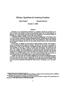
The left-lateral Kunlun fault, located in northern Tibet, was chosen for this study because it experienced a large earthquake during a time period for which ASTER imagery is available. On November 14, 2001, an Ms = 8.1 earthquake occurred causing a 400 km-long surface rupture and as much as 16.3 m of left-lateral strike-slip [16]. This slip is most evident as offset of, and fault scarps developed on, alluvial terraces. Three time separation window cases were considered. These three test cases focus on three different segments of fault. •

•

•

Test Case 1 spans a two-year time window from March 2000 to July 2002. The image pair for this case exhibits extensive erosion due to the long time span of two years. The image pair for this case also has vastly different pointing angles. Test Case 2 has a time separation of two-months, from November 4, 2001 to December 22, 2001. The imagery used in this test case has 13% cloud cover, and one of the images contains snow, both of which caused decorrelation. Test Case 3 has a time separation of thirteen months, between October 2000 and December 2001. The image pair for this case has the least amount of preprocessing problems and the smallest pointing angle difference. Although there is some snow cover and changes in water level along the Kusai Hu lake next to the fault, decorrelation problems were minor. This test case is the only one with a well-defined fault scarp.

For each case, the accuracy of the change detection methods was assessed by comparing the geodetic image processing results to field measurements ([16], Table 2; [14, 28]).


17

Site 1

~3 m

Site 2 ~10 m

Site 3 ~5 m

= Inferred surface Rupture

Before we start registering the corresponding satellite images, we must apply topographic corrections Our objective is to detect the shift between the images with a subpixel accuracy. To achieve this accuracy, we must first apply the corrections that will lead to an exact alignment of the images. One distortion that e need to correct is parallax, which is defined as the apparent shift in the location of an object due to changes in the observers position and, as a result, the relative geometry between the observer and the target. This concept is the same principle on which human stereoscopic vision

18


is based: our right and left eyes view the same scene from slightly different angles, resulting in parallax that we perceive as depth. Thus, topographic parallax is created by the change in the position of a satellite as it scans the uneven surface of the Earth. It results in an apparent shift in the position of terrain features between two overlapping images taken from different angles; see, e.g., [18]. Topography can also impart apparent pixel offsets due to scale changes within the image. In an area of high relief, those parts of the image within valleys will be a greater distance from the observer than those parts on ridge tops. The variable distance between target and observer results in mountaintops having a larger map scale than the valley bottoms, an effect that nonlinearly distorts images. If left uncorrected, this distortion can create apparent pixel shifts when comparing two images. Another apparent pixel offset due to topography stems from the calculation of geographic coordinates. The geographic coordinates of a pixel in an image are calculated from orbital and attitude data and lie on the Earths ellipsoid. Due to the fact the Earth has topography, however, the true latitude and longitude coordinates of a point on the Earths surface will be displaced from its ellipsoidal coordinates. Of the three apparent pixel offsets produced by topography, this last type can cause the greatest apparent shift [29]. All three topographic apparent pixel offsets can be minimized by orthorectifying the image with a DEM. The ortho-rectification process uses the DEM to remove topographic distortions and will re-project the ellipsoidal position of a given pixel to one that better approximates its true coordinates on the Earths surface. In our work, we have applied ortho-rectification techniques to pre-process the images before registering them. All images used in the Kunlun fault test cases are VNIR band 3n images from ASTER level 1B scenes, which has already been through pre-process for sensor artifacts by the ASTER corporation. This band was chosen for two reasons: • •

because it has the highest resolution, and because a sensor model is available [32], which describes the interior and exterior orientations of the image ([18]).

The sensor model is required for the orthorectification process done using the Leica Photogrammetry Suite in 19 ERDAS IMAGINE 8.7 [32]. ASTER VNIR 3b bands were not considered in the test cases due to registration problems. Orthorectification of the 3b images in ERDAS IMAGINE was poor, and there were residual geometric pixel shifts of at least 20 pixels (210 m). The poor orthorectification can be due to either excessive pointing angle differences, or excessive variation in the viewing geometry. The DEM used for orthorectification was the 90-m Shuttle Radar Topography Mission (SRTM; www.jpl.nasa.gov/srtm) DEM. ENVI 4.0 software was used to register the before and after images, and check the orthorectification process done in ERDAS IMAGINE.


19

5 How to Extend the Existing Image Registration Techniques to Images Known with Low Accuracy Problem When we applied the above algorithm to detect the earthquake-caused shift between the pre- and post-earthquake images, we did not get any meaningful shift value. Specifically, the inverse Fourier transform P (x) of the crosscorrelation power spectrum looks random, and its maximum a was attained at values which are very different from the actual shift. Analysis of the problem In the above algorithm, for every frequency ω, we compute the complex-valued product F (ω) · F 0 (ω) and then consider only the phase of this complex value – i.e., equivalently, the value R(ω) – in the further computations. Due to the uncertainty in the satellite geometry and the wobble of the satellite, we only know the images with low accuracy. As a result, the corresponding Fourier transforms F (ω) and F 0 (ω) can also be only determined with low accuracy. So, for every spatial frequency ω, the product F (ω) · F 0 (ω) can also be only determined with low accuracy. How does this low accuracy translate into the accuracy with which we know R(ω)? Let ε be the accuracy with which we know the value of the product. In general, if we multiply a value x known with accuracy ∆x ≈ ε by a number λ, the resulting new value y = λ · x is known with accuracy ∆y = λ · ∆x = λ · ε. Similarly, if we divide the value x by a number λ, then the resulting new value z = x/λ is known with accuracy ∆z = ∆x/λ ≈ ε/λ. In our algorithm, the cross-correlation power spectrum R(ω) is obtained by dividing the product F (ω) · F 0 (ω) by its magnitude |F (ω)| · |F 0 (ω)|. Since we know the product with accuracy ε, we thus know the value R(ω) with accuracy ε/(|F (ω)| · |F 0 (ω)|). As a result: •

for the frequencies ω for which the magnitude is high, we know the corresponding value R(ω) with a reasonable accuracy; • however, for the frequencies ω for which the magnitude is low, the the corresponding value R(ω) is really inaccurate – all noise.

In the above algorithm, when we compute P (x) as the Fourier transform of the function R(ω), we take all the values R(ω) with the same weight. In effect, we are taking the average of several values, some known with reasonable accuracy and some very inaccurate. Not surprisingly, the resulting average is very inaccurate. For example, if we have two measurements of the same quantity whose actual value is 1.0, • •

the first measurement is very accurate and results in 1.05, and the second measurement is way off and results in 5.61,

20


then when we take the average, we get (1.05 + 5.61)/2 = 3.33 in which the noisy values dominated the accurate ones. How to make resulting estimate more accurate: an idea In view of the above analysis, to make the measurements more accurate, we should: assign less weight to less accurate values R(ω), i.e., values for which the magnitude |F (ω)| · |F 0 (ω)| is small, and • assign more weight to more accurate values R(ω), i.e., values for which the magnitude |F (ω)| · |F 0 (ω)| is large. •

The simplest way is to assign weight 0 to less accurate measurements and weight 1 to more accurate measurements. In other words, the simplest way to implement this idea is: • •

to fix some threshold, and for all the frequencies for which the magnitude |F (ω)| · |F 0 (ω)| is below this threshold, set R(ω) to 0.

A natural idea is to select, as a threshold, a certain portion of the largest (or mean) value of |F (ω)| · |F 0 (ω)|. As a result, we arrive at the following algorithm. Registration algorithm for images that are known with low accuracy: first attempt To find the shift a between the two images: first, we apply FFT to the original images I(x) and I 0 (x) and compute their Fourier transforms F (ω) and F 0 (ω); • on the second step, we do the following: – we find the mean value m of the product |F (ω)| · |F 0 (ω)|; – we set the threshold to be a certain portion of the mean, i.e., to α · m for some α > 0; – for those frequencies for which |F (ω)| · |F 0 (ω)| ≥ α · m, we compute the value R(ω) by using the formula (17); – for other frequencies, we set R(ω) = 0; • on the third step, we apply the inverse FFT to the function R(ω) and compute its inverse Fourier transform P (x); • finally, on the fourth step, we determine the first approximation to the desired shift a as the point for which |P (x)| takes the largest possible value, and then do the interpolation by using formulas (18)–(19). •

Empirically, the best value for the parameter α turned out to be 10−3 .


21

How to improve the above algorithm We have mentioned that due to the inaccuracy, it is very difficult to detect the lateral shift. In general, when measurements are not very accurate, a natural way to increase the accuracy is to perform repeated measurements and then average the measurement results. With respect to images, this means that we have to consider more pixels, i.e., large parts of the compared image, corresponding to larger sliding window size. However, the problem is that the lateral shift differs from location to location: its value decreases as we get farther away from the fault. So, when we increase the window size, instead of processing several pixels with the same shift (which would have helped), we instead bring together pixels corresponding to different values of lateral shift. Good news is that while the magnitude of the lateral shift is different at different pixels, the direction of this shift remains largely the same. So, at the first stage of our analysis, we take a large sliding window (larger that 75 × 75 pixels, where 1 pixel is ≈ 15 m), and use the above algorithm to determine the direction of the lateral shift. Once the direction at different locations is determined, we can now take smaller sliding windows (40 × 40 pixels), and determine the magnitudes of the lateral shift. The directions can also be obtained from these smaller windows, but these direction are determined from he analysis of fewer pixels and are, thus, much less accurate than the directions obtained form the analysis of a larger window. Thus, to get the best results, we combine the direction obtained form the analysis of a larger window with the magnitude obtained from the smaller window. In other words, we need to apply the above algorithm twice: • •

first, with a larger sliding window, to find the direction of the lateral shift; then, with a smaller sliding window, to find the shift’s magnitude.

Finally, we combine the direction obtained from a larger window with the magnitude obtained from a smaller window. Thus, we arrive at the following algorithm: Registration algorithm for images that are known with low accuracy: final description To find the shift a between the two images at a given location x = (x1 , x2 ), we select the two window sizes δ < ∆. Then: • First, we apply the above “first attempt” algorithm to subimages corresponding to a larger box (window) [x1 − ∆, x1 + ∆] × [x2 − ∆, x2 + ∆] def a around x. Based on the resulting shift a, we find the direction e = kak def p 2 2 of the actual (unknown) lateral shift (here kak = a1 + a2 ).

22

•


Then, we apply the above “first attempt” algorithm to subimages corresponding to a smaller box (window) [x1 − δ, x1 + δ] × [x2 − δ, x2 + δ] around def

x. Based on the resulting shift a, we find the shift’s magnitude M = kak. • Finally, we combine the direction e obtained from a larger window with the magnitude m obtained from a smaller window into the estimate M · e for the desired shift. This is the new FFT-based algorithm that we propose to use for registering images know with low accuracy.

6 Results of Applying the New Image Registration Algorithm To test our new algorithm, we applied it to all three test zones. All test cases display good results in the near field of the faulted area; the accuracy with which we can determine the shift decreases as we move to distal areas. Test Case 2 gives the best results, with a measured lateral displacement of 4.5 ± 0.4 m with left-lateral slip and an average slip direction of 270◦ . This magnitude is similar to the 4.6-4.8 m displacement of a gulley measured by Lin et al. [16] (site 2 in Table 2 from [16]), and the sense and slip direction are consistent with the known trace and kinematics of the Kunlun fault. Test Case 3 is fairly consistent in direction, with left lateral movement and an average slip direction of 265◦ . However, the magnitude obtained from this analysis, ≈ 8.4 m, is a much cruder approximation to the 5.7 m of displacement measured by Lin et al. [16] (site 3 in Table 2). This could be attributed to the long 13-month time separation window during which non-earthquake terrain change occurred, such as changes in the water level in Kusai Hu lake. Test Case 1 results in left-lateral slip with an azimuth of 268◦ in the nearfield of the fault and a magnitude of ≈ 8.3 m. The sense of slip and azimuth are consistent with field observations, but assessing the accuracy of the resulting magnitude is less straightforward. The closest of the Lin et al. [16] field sites is site 7. Several offset features were measured here, with displacements ranging from 3.3 m on a road to 6.8 m on a stream channel. The latter is similar, as is the field measurement at another nearby locality, site 6, where Lin et al. [16] report 7.2 m of displacement on a stream channel.

7 Conclusions and Future Work Main conclusion Our results have shown that the new algorithm provides a good reconstruction of shift between the two images.


23

Using better DEM Future work needed includes improving the pre-processing protocol. This improvement is needed in order to fully remove any residual apparent pixel offsets and to optimize the true pixel offsets. This can be accomplished by using a 30-m DEM instead of a 90-m DEM in the ortho-rectification process. A higher-resolution DEM can be obtained from aerial photographs or LIDAR, among other sources, but will require an investment of time and resources. By using a DEM with a higher resolution, the elevation uncertainty can be improved, thus lowering the apparent pixel offsets caused by parallax. Comparing images of different type Future work should also include applying the change detection procedures developed in this thesis to heterogenous input imagery, for instance, a combination of an ASTER “after” image with a Landsat TM scene or aerial photographs as “before” images. By using a heterogonous pair of input imagery, a greater number of possible image candidates can be used to do change detection. In addition, since Landsat images and aerial photographs are available for times prior to the beginning of ASTER image acquisition, using heterogeneous datasets can also lengthen the time separation windows that can be considered. This can be especially useful for monitoring terrain change due to slow processes such as glacier movement. It can also make possible the study of events that occurred before ASTER was launched. Comparing images with gridded data sets The algorithms desscribed in this paper should be able to detect lateral movements in any kind of registered imagery. Thus, the possibility exists to apply these methods to gridded gravity and other geophysical data. Use redundancy of ASTER images As an effort to improve our knowledge of ASTER attitude parameters and to minimize residual apparent pixel offsets during ortho-rectification, as well as improve the performance of the change detection techniques with ASTER data, it may be possible to exploit the redundancy in the ASTER VNIR imagery [29]. The redundancy provided by the ASTER is possible due to its stereo capability, a feature which, given two ASTER scenes, essentially provides four independent sets of images to process for terrain displacement. Given a single “before” scene and a single “after” scene, there are a total of four unique permutations of image pairs that can be used as input to a terrain change detection algorithm. All else being equal, each permutation should result in identical terrain change measurements. Differences in the estimates, however, can be reconciled by optimization of poorly-constrained parameters such as the satellite attitude (e.g., roll, pitch, and yaw). We can also use the fact that the images are multi-spectra [3, 4] (see also Appendix).

24


Towards more accurate shift, rotation, and scaling It is important to find the lateral shift between pre- and post-earthquake images. Once this relative shift is determined, it is desirable to shift one of the images to see what changes occurred. The difficulty is that the shift is subpixel, so when we shift, we move away from the original rectangular grid: the brightness values of the first image were given on a grid, but the values of the shifted image are on the shifted points, which are in between the points of the original grid. Thus, to adequately compare the two images pixel-by-pixel, we must interpolate the brightness values from the shifted grid points (at which we know the brightnesses of the shifted first image) to the original grid point (at which we know the brightnesses of the second image). In the above text, we used bilinear interpolation to actually perform the corresponding geometric transformation (shift, rotation, or scaling). This methods is efficient – it requires only a few computations per pixel – but because of its localized character, it is not always accurate. It is well known that the more points we use for interpolation, the better results we can achieve. Ideally, interpolation should use all the available points. Such methods have indeed been developed based on efficient FFT-based implementations of socalled chirp-z transform – a generalization of Fourier transform [27]. It is desirable to apply these methods to geosciences-related images. Methods from [27] can perform shifts and scalings in an arbitrary rectangular grid, but efficient rotation techniques are only available for the case when we have a rectangular grid with exactly the same step sizes in two dimensions, i.e., when the grid is actually a square grid. For satellite images, it is often not the case. To handle such situations, we must thus: • • •

first, interpolate from the original rectangular grid to the square grid; then, perform the rotation in the square grid, and finally, interpolate the rotated image back into the original rectangular grid.

Towards explicit representation of interval and fuzzy uncertainty in images In the current image processing, an image is represented as follows: for each e pixel x, we describe the approximate value I(x) of the brightness at this pixel. It is desirable to describe not only this approximate value, but also the accuracy with which we know this value. For example, if for each pixel, we know the guaranteed upper bound ∆(x) for the inaccuracy of the corresponding brightness value, this means that at each pixel x, the actual (unknown) value of the brightness I(x) belongs to the interval def e e + ∆(x)]. I(x) = [I(x), I(x)] = [I(x) − ∆(x), I(x) In a more realistic situation, instead of the guaranteed bound, we may have def e with different different values which bound the difference ∆I(x) = I(x)− I(x)


25

degrees of certainty. In other words, for every pixel x, we have nested intervals corresponding to different degrees of certainty – i.e., in effect, a fuzzy value I(x). A fuzzy-valued image is thus simply a nested (layered) family of intervalvalued images. How can we process such interval and fuzzy images? To transform (shift, rotate, scale) an interval image [I(x), I(x)], it is sufficient to rotate the corresponding endpoint images I(x) and I(x). To transform a fuzzy image, it is sufficient to rotate the corresponding interval images layer-by-layer.

Acknowledgments This work was supported in part by NASA under cooperative agreement NCC5-209, NSF grants EAR-0225670 and DMS-0532645, by Army Research Lab grant DATM-05-02-C-0046, by the Star Award from the University of Texas System, and by the Texas Department of Transportation grant No. 0-5453. The authors are very thankful to the anonymous referees for their thorough analysis and valuable suggestions.

References 1. Abrams M, Hook S, Ramachandran B (2002) Aster User Handbook, NASA Jet Propulsion Laboratory, Pasadena, California 2. Adidhela JE (2004) Using FFT-based Data Processing Techniques to Characterize Asphaltic Concrete Mixtures, Master Thesis, Department of Computer Science, University of Texas at El Paso 3. Araiza R (2003) Optimal FFT-Based Algorithms for Referencing MultiSpectral Images, Master Thesis, Department of Computer Science, University of Texas at El Paso 4. Araiza R, Xie H, Starks SA, Kreinovich V (2002) Automatic Referencing of Multi-Spectral Images. In: Proceedings of the IEEE Southwest Symposium on Image Analysis and Interpretation, Santa Fe, New Mexico, USA, April 7–9, 2002, pp. 21–25 5. Brown LG (1992) A Survey of Image Registration Techniques. ACM Computing Surveys 24(4):325–376 6. Burgmann R, Rosen PA, Fielding EJ (2000) Synthetic Aperture Radar Interferometry to Measure Earth’s Surface Topography and Its Deformation. Annu. Rev. Earth Planet. Sci. 28:169–209 7. Cormen TH, Leiserson CE, Rivest RV, Stein C (2001) Introduction to Algorithms. MIT Press, Cambridge, Massachusetts 8. Crippen RE, Blom RG (1991) Measurement of Subresolution Terrain Displacements using SPOT Panchromatic Imagery. In: Proceedings of the 1991 International Geoscience and Remote Sensing Symposium IGARSS’91 “Remote Sensing: Global Monitoring for Earth Management”, June 3–6, 1991, Vol. 3, pp. 1667–1670

26


9. Dominguez S, Avouac JP, Michel R (2003) Horizontal coseismic deformation of the 1999 Chi-Chi earthquake measured from SPOT satellite images: Implications for the seismic cycle along the western foothills of central Taiwan. Journal of Geophysical Research 108(B2):2083 10. Feigl KL, Sarti F, Vadon H, McClusky S, Ergintav S, Durand P, Burgmann R, Rigo A, Massonnet D, Reilinger R (2002) Estimating Slip Distribution for the Izmit Mainshock from Coeseismic GPS, ERS-1, RADARSAT, and SPOT Measurements. Bulletin of the Seismological Society of America 92(1) 138–160 11. Garcia F, Araiza R, Rzycki B (2000) Towards optimal mosaicking of multispectral images. In: Proc. 2nd Nat’l NASA Student Conference, Nashville, Tennessee, April 7–10, 2000. 12. Gibson S (1999) An optimal FFT-based algorithm for mosaicking images, Master Thesis, Department of Computer Science, University of Texas at El Paso 13. Gibson S, Kreinovich V, Longpr´e L, Penn B, Starks SA (2001) Intelligent Mining in Image Databases, With Applications to Satellite Imaging and to Web Search. In: Kandel A, Bunke H, Last M (eds.), Data Mining and Computational Intelligence, Springer-Verlag, Berlin, 309–336 14. King G, Klinger Y, Bowman D, Tapponnier P (2005) Slip-Partitioned Surface Breaks for the Mw = 7.8 2001 Kokoxili Earthquake, China. Bulletin of the Seismological Society of America 95:731–738 15. Lang HR (1999) Algorithm Theoretical Basis Document for ASTER Digital Elevation Models (Standard Product AST14), Version 3.0: NASA Jet Propulsion Laboratory 16. Lin A, Fu B, Guo J, Qingli Z, Guangming D, He W, Zhao Y (2002) Coseismic strike-slip and rupture length produced by the 2001 Ms = 8.1 central Kunlun earthquake. Science 296(5575):2015–2017 17. Michel R, Avouac JP (2002) Deformation due to the 17 August 1999 Izmit, Turkey, earthquake measured from SPOT images. Journal of Geophysical Research 107(B4) 18. Mikhail EM, Bethel JS, McGlone JM (2001) Introduction to Modern Photogrammetry. New York, John Wiley & Sons, Inc. 19. Osegueda R, Keller GR, Starks SA, Araiza R, Bizyaev D, Kreinovich V (2004) Towards a General Methodology for Designing Sub-Noise Measurement Procedures. In: Proceedings of the 10th IMEKO TC7 International Symposium on Advances of Measurement Science, St. Petersburg, Russia, June 30–July 2, 2004, Vol. 1, pp. 59–64 20. Peltzer G, Crampe F, Rosen P (200) The Mw = 7.1, Hector Mine, California earthquake: surface rupture, surface displacement, and fault slip solution from ERS SAR data. Earth and Planetary Sciences 333:545–555 21. Reddy BS, Chatterji BN (1996) An FFT-based technique for translation, rotation, and scale-invariant image registration. IEEE Transactions on Image Processing 5(8):1266–1271 22. Riazanoff S (2002) SPOT Satellite Geometry Handbook. SPOT Image 23. Schiek CG (2004) Terrain change detection using aster optical satellite imagery along the Kunlun fault, Tibet, Master Thesis, Department of Geological Sciences, University of Texas at El Paso 24. Srikrishnan S (2002) Referencing noisy images: complexity of the problem, analysis and efficient implementation of the Fast Fourier approach, Master Thesis, Department of Computer Science, University of Texas at El Paso


27

25. Srikrishnan S, Araiza R, Xie H, Starks SA, Kreinovich V (2001) Automatic referencing of satellite and radar images. In: Proceedings of the 2001 IEEE Systems, Man, and Cybernetics Conference, Tucson, Arizona, October 7–10, 2001, pp. 2176–2181 26. Starks SA, Nazarian S, Kreinovich V, Adidhela J, Araiza R (2004) Using FFTBased Data Processing Techniques to Characterize Asphaltic Concrete Mixtures. In: Proceedings of the 11th IEEE Digital Signal Processing Workshop DSP’04, Taos Ski Valley, New Mexico, August 1–4, 2004, pp. 241–245 27. Tong R, Cox RW (1999) Rotation of NMR images using the 2D chirp-z transform. Magnetic Resonance in Medicine 41:253–256 28. Van der Woerd J, Meriaux AS, Klinger Y, Ryerson FJ, Gaudemer Y, Tapponnier P (2002) The 14 November 2001, Mw = 7.8 Kokoxili Earthquake in Northern Tibet (Qinghai Province, China). Seismological Research Letters 73(2):125–135 29. Van Puymbroeck N, Michel R, Binet R, Avouac JP, Taboury J (2000) Measuring earthquakes from optical satellite images. Applied Optics 39(20):3486–3494 30. Xie H, Hicks N, Keller GR, Huang H, Kreinovich V (2000) Automatic image registration based on a FFT algorithm and IDL/ENVI. In: Proceedings of the ICORG-2000 International Conference on Remote Sensing and GIS/GPS, Hyderabad, India, December 1–4, 2000, Vol. 1, pp. 397–402 31. Xie H, Hicks N, Keller GR, Huang H, Kreinovich V (2003) Implementation, test, and analysis of an automatic image registration algorithm based on FFT and IDL/ENVI. Computers and Geosciences 29(8):1045–1055 32. Yu J, Cowgill E, Healy S (2003) Digital Stereomapping in Imagine Orthobase, California Institute of Technology, pp. 1–10 33. Zitov´ a B, Flusser J (2003) Image registration methods: a survey. Image and Vision Computing 21:977–1000.

Appendix: Registration of Multi-Spectral Satellite Images Formulation of the problem With the new generation of multi-spectral satellites, for each area, we have several hundred images which correspond to different wavelengths. At present, when we register two images, we only use one of the wavelengths and ignore the information from the other wavelengths. It is reasonable to decrease the registration error by using images corresponding to all possible wavelengths in registration. Similarly, in detecting the known text in colored web images, we would like to take into consideration all color components. In this appendix, we present an algorithm for such optimal registration. Derivation of the new algorithm For multi-spectral imaging, instead of a single image I(ω), we get several images Ii (ω), 1 ≤ i ≤ n, which correspond to different wavelengths. So, we have two groups of images:

28

• •


the images Ii (ω) which correspond to one area, and the images Ii0 (ω) which correspond to an overlapping area.

Let us first consider the case when two images differ only by some (unknown) shift a. For every wavelength i, the corresponding two images Ii (x) and Ii0 (x) differ only by shift, i.e., Ii0 (x) = Ii (x + a). Therefore, for every wavelength i, their Fourier transforms Z Z 1 Fi (ω) = · Ii (x) · e−2π·i·(x·ω) dx1 dx2 , 2π Z Z 1 · Ii0 (x) · e−2π·i·(x·ω) dx1 dx2 , Fi0 (ω) = 2π are related by the formula: Fi0 (ω) = e2π·i·(ω·a) · Fi (ω).

(20)

In the ideal no-noise situation, all these equations are true, and we can determine the value r = e2π·i·(ω·a) from any of these equations. In the real-life situations, where noise is present, these equations (20) are only approximately true, so we have the following problem instead: find r for which, for all i, Fi0 (ω) ≈ r · Fi (ω).

(21)

and which satisfies the condition (7). We would like to get the best estimate for r among all estimates which satisfy the condition (7). To get the optimal estimate, we can use the Least Squares Method, according to which, for each estimate r and for each i, we define the error Ei = Fi0 (ω) − r · Fi (ω) (22) with which the condition (21) is satisfied. Then, we find among all estimates which satisfy the additional condition (7), a value r for which the sum of the squares |E1 |2 + . . . + |En |2 = E1 · E1∗ + . . . + En · En∗ of these errors is the smallest possible. The square |Ei |2 of each error Ei can be reformulated as follows: ¢ ¡ ∗ Ei · Ei∗ = (Fi0 (ω) − r · Fi (ω)) · F 0 i (ω) − r∗ · Fi∗ (ω) = ∗

∗

Fi0 (ω)·F 0 i (ω)−r∗ ·Fi∗ (ω)·Fi0 (ω)−r·Fi (ω)·F 0 i (ω)+r·r∗ ·Fi (ω)·Fi∗ (ω). (23) We need to minimize the sum of these expressions under the condition (7). For this conditional minimization, we will use the Lagrange multipliers technique, which leads to the following unconditional minimization problem: n X ¡ 0 ∗ Fi (ω) · F 0 i (ω) − r∗ · Fi∗ (ω) · Fi0 (ω)− i=1


29

¢ ∗ r · Fi (ω) · F 0 i (ω) + r · r∗ · Fi (ω) · Fi∗ (ω) + λ · (r · r∗ − 1) → min .

(24)

Differentiating (24) relative to r∗ , we get the following linear equation: −

n X

Fi∗ (ω) · Fi0 (ω) + r ·

i=1

n X

Fi (ω) · Fi∗ (ω) + λ · r = 0.

(25)

i=1

From this equation, we conclude that n X

r=

Fi∗ (ω) · Fi0 (ω)

i=1 n X

.

(26)

Fi (ω) · Fi∗ (ω) + λ

i=1

The coefficient λ can be now determined from the condition that the resulting n X value r should satisfy the equation (7). The denominator Fi (ω)·Fi∗ (ω)+λ i=1

of the equation (26) is a real number, so instead of finding λ, it is sufficient to find a value of this denominator for which |r|2 = 1. One can easily see that to achieve this goal, we should take, as this denominator, the magnitude of the numerator, i.e., the value ¯ ¯ n ¯X ¯ ¯ ¯ ∗ 0 Fi (ω) · Fi (ω)¯ . (27) ¯ ¯ ¯ i=1

For this choice of a denominator, the formula (25) takes the following final form: n X Fi∗ (ω) · Fi0 (ω) def ¯. r = R(ω) = ¯¯ i=1 n ¯ ¯X ∗ ¯ Fi (ω) · Fi0 (ω)¯ ¯ ¯ ¯

(28)

i=1

So, for multi-spectral images, in the presence of noise, instead of using the exact ratio (4), we should compute, for every ω, the optimal approximation (28). Hence, we arrive at the following algorithm: A new algorithm for determining the shift between two multi-spectral images If we have images Ii (ω) and Ii0 (ω) which correspond to different wavelengths, then, to determine the shift a between these two multi-spectral images, we do the following: •

first, we apply FFT to the original images Ii (x) and Ii0 (x) and compute their Fourier transforms Fi (ω) and Fi0 (ω);

30


•

on the second step, we compute the ratio (28) – setting the value to 0 if the denominator is below the threshold; • on the third step, we apply the inverse FFT to the ratio R(ω) and compute its inverse Fourier transform P (x); • finally, on the fourth step, we determine the first approximation to the desired shift a as the point for which |P (x)| takes the largest possible value, and perform the interpolation (18)–(19) to find the actual shift with subpixel accuracy. For rotation and scaling, we can use the same reduction to shift as for mono-spectral images. As a result, we get the desired values of shift, rotation, and scaling; hence, we get the desired registration.

Images with Uncertainty: Efficient Algorithms for Shift ... - UTEP CS

Images with Uncertainty: Efficient Algorithms for Shift ... - UTEP CS

Suggest Documents