Imaging and computational considerations for image ...

Advances in Water Resources 116 (2018) 127–144

Contents lists available at ScienceDirect

Advances in Water Resources journal homepage: www.elsevier.com/locate/advwatres

Imaging and computational considerations for image computed permeability: Operating envelope of Digital Rock Physics Nishank Saxena∗, Amie Hows, Ronny Hofmann, Faruk O. Alpak, Justin Freeman, Sander Hunter, Matthias Appel Shell International Exploration & Production, Houston, TX, USA

a r t i c l e Keywords: Digital rock Permeability Petrology Numerical solutions REV

i n f o

a b s t r a c t This study defines the optimal operating envelope of the Digital Rock technology from the perspective of imaging and numerical simulations of transport properties. Imaging larger volumes of rocks for Digital Rock Physics (DRP) analysis improves the chances of achieving a Representative Elementary Volume (REV) at which flowbased simulations (1) do not vary with change in rock volume, and (2) is insensitive to the choice of boundary conditions. However, this often comes at the expense of image resolution. This trade-off exists due to the finiteness of current state-of-the-art imaging detectors. Imaging and analyzing digital rocks that sample the REV and still sufficiently resolve pore throats is critical to ensure simulation quality and robustness of rock property trends for further analysis. We find that at least 10 voxels are needed to sufficiently resolve pore throats for single phase fluid flow simulations. If this condition is not met, additional analyses and corrections may allow for meaningful comparisons between simulation results and laboratory measurements of permeability, but some cases may fall outside the current technical feasibility of DRP. On the other hand, we find that the ratio of field of view and effective grain size provides a reliable measure of the REV for siliciclastic rocks. If this ratio is greater than 5, the coefficient of variation for single-phase permeability simulations drops below 15%. These imaging considerations are crucial when comparing digitally computed rock flow properties with those measured in the laboratory. We find that the current imaging methods are sufficient to achieve both REV (with respect to numerical boundary conditions) and required image resolution to perform digital core analysis for coarse to fine-grained sandstones.

1. Introduction Digital Rock Physics (DRP) analyses include image-based computation of flow properties of reservoir rocks, subsurface hydrogeological properties, mechanical properties such as elastic moduli, electromagnetic properties, thermal properties, and other averaged quantities of porous media. DRP also aims to improve our understanding of how multiphysics evolves from pore-scale to meso‑scale. DRP complements, and in some cases, replaces, the need for relatively slow laboratorybased measurements and empirical rock property models. DRP can lead to more, faster and cheaper core analysis, and generate early data for project acceleration. Furthermore, in the last decade or so, DRP has evolved into an active field of multidisciplinary research (Adler et al., 1990; Andrä et al., 2013a,b; Arns et al., 2005, 2002; Berryman and Blair, 1986; Blunt et al., 2013; Dvorkin et al., 2011, 2008; Kanckstedt et al., 2001; Knackstedt et al., 2008; Knackstedt et al., 2009; Øren et al., 2006; Saenger, 2008; Saenger et al., 2011; Sain et al., 2014; Saxena and Mavko, 2016; Saxena et al., 2017b; Saxena et al., 2017c).

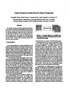
We discuss imaging considerations of rocks to compute transport properties in terms of two fundamental quantities (1) the ratio of dominant pore throat size to voxel size, and (2) the ratio of field of view of the acquired image and a measure of grain size. The first constraint is linked to quality of image resolution whereas the second constraint is related to achieving the Representative Elementary Volume (REV) for numerical simulations of flow properties. Due to the finiteness of modern imaging detectors (e.g., X-ray micro computed tomography), there exists a tradeoff between achieving REV and resolving pore throats. As an illustration of this tradeoff, consider the example in Fig. 1. The same rock is imaged with different voxel sizes (e.g., 0.3, 2.4, and 9.80 μm) such that all acquired images have 1024 voxels on each side. These are transmitted light optical microscope from a thin section that has 30 μm thickness. Also shown are the corresponding segmented images. We note that the pores in the fine resolution (i.e., smaller voxel size) image are very well resolved but the image is unlikely to be large enough (physically) to achieve the REV, on the other hand, the coarse resolution image is probably the REV but the pores are not resolved.

∗

Corresponding author. E-mail addresses: [email protected] (N. Saxena), [email protected] (A. Hows), [email protected] (R. Hofmann), [email protected] (F. O. Alpak), [email protected] (J. Freeman), [email protected] (S. Hunter), [email protected] (M. Appel). https://doi.org/10.1016/j.advwatres.2018.04.001 Received 28 December 2017; Received in revised form 22 March 2018; Accepted 2 April 2018 Available online 4 April 2018 0309-1708/© 2018 Elsevier Ltd. All rights reserved.

N. Saxena et al.

Advances in Water Resources 116 (2018) 127–144

Fig. 1. Top: Two-dimensional images of size 10242 acquired at three different voxel sizes (as shown in the legend). Middle: segmented images corresponding to images (top) of different voxel sizes. Bottom: same segmented area from the three images of different voxel sizes are shown in the orange box. (For interpretation of the references to color in this figure legend, the reader is referred to the web version of this article.)

To this end, we first analyze imaging considerations to sufficiently resolve pore throats. Subsequently, we establish constraints for the REV by analyzing the variation in various rock properties calculated using pore morphology-based methods with increasing rock volume. Furthermore, we analyze the variation in computed permeability for volumes of various sizes using four different numerical flow simulation approaches with multiple boundary conditions. Based on our findings, we discuss the minimum considerations for imaging rocks to calculate reliable digital rock properties estimations.

2. Limits imposed due to imaging Image quality, voxel size, and limited field of view, all put constraints on flow properties that can be calculated using the Digital Rock technology. Two dimensionless parameters that describe these effects are (1) the ratio of dominant pore throat size to voxel size (NI ), and (2) the ratio of field of view of the acquired image and effective grain size (NREV ). We define these two parameters as follows: 𝑁𝐼 =

Fig. 2. Grain and pore size (diameter) ratio versus porosity. Data from petrographic interpretation for many siliciclastic rocks are shown in gray circles. The area above the red line corresponds to Deff /DD > 40. (For interpretation of the references to color in this figure, the reader is referred to the web version of this article.)

𝐷𝐷 , Δ𝑥

𝑁𝑅𝐸𝑉 = 128

𝐿 𝐷𝑒𝑓 𝑓

(1)

(2)

N. Saxena et al.

Advances in Water Resources 116 (2018) 127–144

(where 𝜎 is mercury-air surface tension ≈ 480 [dyne/cm] and 𝜃 is the contact angle ≈ 40°; if PD is expressed in psi and DD is expressed μm then 2𝜎cos 𝜃 ≈ 213). The entry pressure PD can be directly measured in a mercury injection capillary pressure (MICP) experiment (Swanson, 1981a; Thomeer, 1983, 1960). Alternatively, PD and DD can also be inferred using image-based simulations (Hilpert and Miller, 2001). Many rocks exhibit dual pore structures (Desbois et al., 2011; Hemes et al., 2015; Houben et al., 2013) and cannot be sufficiently described by a single dominant pore throat, in such cases multiple NI parameters must be used. Deff is the effective grain diameter for permeability (Rumpf and Gupte, 1971) defined as ∫ 𝐷 𝑛(𝐷)𝑑𝐷 2

𝐷𝑒𝑓 𝑓 =

∫ 𝐷 𝑛(𝐷)𝑑𝐷 3

,

(3)

where, n(D) is the number distribution of each grain diameter. The effective grain diameter Deff can be calculated using grain size distribution measured in a laboratory (e.g., sieve analysis) and can also be inferred using image-based algorithms. Therefore, both parameters NI and NREV can be estimated directly using a 3D digital rock image. The effective grain diameter (Deff ) is a complicated function of the entry pore throat size (DD ). Such a relationship also depends on many other textural parameters, including porosity, coordination number, rock type, and grain shape. The parameter NI describes the quality of image resolution whereas the parameter NREV describes the number of grains captured in an image to sample the desired heterogeneity. In an ideal scenario, we would like to image as fine and as large as possible (i.e., NI → ∞ and NREV → ∞) but this is simply not possible due to limitations of imaging techniques. Most imaging devices (e.g., X-ray micro computed tomography (micro-CT)) can accommodate only a predefined number of voxels (M3 ). Even through the micro-CT detectors are rapidly improving, the current

Fig. 3. Region of reliable permeability that can be computed using the DRP technology using images of voxel sizes 1 μm, 2 μm, and 4 μm are shown in cyan, green, and blue, respectively. Region for 2D thin sections (0.1 μm voxel size) is shown in red. Laboratory data from an internal Shell database for many siliciclastic rocks are shown in gray circles. (For interpretation of the references to color in this figure legend, the reader is referred to the web version of this article.)

In Eqs. (1) and (2), Δx is image voxel size, L is the field of view or length of the digital rock (in any direction), DD is the pore throat size corresponding to the so-called mercury “entry pressure” denoted here by PD . Parameters PD and DD are related by PD = 2𝜎cos 𝜃/DD

Fig. 4. Variation of permeability with changes in voxel size. 129

N. Saxena et al.

Advances in Water Resources 116 (2018) 127–144

psi), and G is a dimensionless pore shape parameter (G varies between 0.1–0.2 for siliciclastic rocks and 0.2–0.3 for carbonates rocks). Eq. (4) can also be written in terms of diameter of the entry pore throat DD (in μm) as ( ) 𝜙𝐷𝐷 2 𝑘 = 38, 068G−4∕3 . (5) 213 Substituting Eq. (1) in Eq. (5) we obtain ( ) 𝜙Δ𝑥𝑁𝐼 2 𝑘 = 38068G−4∕3 . 213

(6)

The smallest possible value of parameter NI is simply 1 (when pore throat size is same as the voxel size). Such a case would correspond to a heavily pixelated digital rock image. Substituting NI = 1 in Eq. (6), 2 μm voxel size (i.e., Δx= 2 μm), and 20% porosity (i.e., 𝜙 = 0.2), we calculate a permeability of 1 mDarcy, that is the smallest permeability that can be calculated for such a digital image which still somehow contains a network of connected pores. For this analysis we assume G = 0.2. Assuming a minimum value of NI = 10, an image of voxel size Δx = 2 μm and 𝜙 = 0.2, yields k = 100 mDarcy as the smallest permeability that can be reliably calculated using an image of 2 μm voxel size. If the actual permeability of the rock in question is lower than 100 mDarcy, then an image of higher resolution should be acquired. Any computation carried out on an image or below the total porosity and permeability trend defined by Eq. (6) will need to be corrected. Here we assumed a minimum value of NI = 10. However, in practice, the required minimum value of NI will increase with complexity of the pore shape; this will be addressed in a future study. We must note that although Thomeer’s permeability relation in Eq. (4) is an empirical relation, this relation has been extensively calibrated using laboratory-measured data (MICP and brine permeability) and petrographic interpretations from many reservoir sandstone rocks it yields results that agree with laboratory-measured brine permeability within a factor of 2. Similar analysis can be performed using other empirical models (e.g., Swanson, 1981b). Similar to the analysis above, the minimum required value of parameter NREV imposes a loose upper bound on image-computed permeability. This is because there is an upper limit on the size of grains that can be fit in an image which naturally translates to an upper bound on permeability. To illustrate this, we again use Thomeer’s permeability relation. In order to use the same permeability relation in Eq. (5), for convenience, we consider the following relation between DD and Deff :

Fig. 5. Computed permeability for a rock scanned at two different resolutions (voxel size: 4 and 8 μm). The computed value is normalized with the laboratorymeasured brine permeability.

detectors capture fewer than 20003 voxels (i.e., M < 2000) in the lateral direction. Therefore, the REV can be achieved by sampling larger rock volumes but only at the expense of coarser image resolution. One can choose to image a larger field of view (i.e., physical dimension) at coarse resolution or image a smaller piece of rock at higher resolution. Thus, there is a tradeoff between sampling sufficiently many grains/pores to achieve the REV and still resolve pore throats to maintain quality of numerical simulations on images. Given this trade off, we will now illustrate how the two imaging parameters NI and NREV impact the computed permeability using simple empirical permeability relation. The minimum value of parameter NI that is needed to capture sufficient structural complexity of rock microstructure and maintain simulation quality puts a loose lower bound on permeability that can be reliably calculated using an image. This is because permeability depends on physical dimensions of pore throat, which must be larger than the voxel size to be visible in an image. Using an empirical relation between pore throat size and permeability, we will now illustrate how the parameter NI (that depends on both voxel size Δx and pore throat size DD ) controls the lowest permeability that can be reliably calculated using a digital rock image. Thomeer (1983) proposed the following empirical relation that relates brine permeability to entry pressure PD (from a MICP measurement): ( )2 𝑘 = 38, 068G−4∕3 𝜙∕𝑃𝐷 . (4)

𝐷𝑒𝑓 𝑓 ∕𝐷𝐷 = 𝑎𝜙𝑏

(7)

The relation in Eq. (7) is motivated by observations from analyzing an internal Shell database of laboratory measurements of MICP and laboratory-measured effective grain size in siliciclastic rocks (Fig. 2). The relevance of the red line corresponding to Deff /DD > 40 is discussed in a later section. It is important to note that the empirical relation in Eq. (7) is not universal and is only used here for the sake of illustration. Substituting Eq. (7) into Eq. (5), we obtain a loose upper bound on permeability ( )2 𝜙𝑀Δ𝑥 𝑘 = 38068G−4∕3 . (8) 𝑏 213𝑎𝜙 𝑁𝑅𝐸𝑉 Assuming NREV = 5, M = 1400, G = 0.2, a = 0.5, b = −2, Δx = 2 μm, and 𝜙 = 0.2, yields k = 570 mDarcy as the largest permeability that can be reliably calculated using an image of 2 μm voxel size so that REV requirements are satisfied. Therefore, the range of reliable permeability that can be calculated using an image of 2 μm voxel size for a 20% porosity rock is 100–570 mDarcy, assuming the parameters described above. This range is only a rough guide but represents the optimum working range for DRP simulations. Fig. 3 shows the region (defined by Eqs. (6) and (8)) of permeability that can be calculated using images of voxel sizes 1, 2, and 4 μm as a function of porosity, assuming M = 1400, NREV = 5, and NI = 10. Also, shown in Fig. 3 is the region spanned by high

In Eq. (4), k is absolute permeability (in mDarcy), 𝜙 is total rock porosity (in fraction), PD is the entry pressure for mercury injection (in 130

N. Saxena et al.

Advances in Water Resources 116 (2018) 127–144

Fig. 6. Gray-scale micro-CT images of digital rocks.

Fig. 7. Segmented rocks (10,243 ) and sphere pack.

131

N. Saxena et al.

Advances in Water Resources 116 (2018) 127–144

Fig. 8. 2D slices of watershed segmented micro-CT images of rocks. Grain size distributions are also shown.

3. Resolving pore throats We now estimate the minimum value of NI needed to resolve pore throats and compute properties that are nearly independent of how an image is discretized. To establish the variation of porosity and permeability for rocks with a change in voxel size, we down sample a high-resolution rock, originally acquired with voxel size of 0.3 μm, using bi-cubic interpolation. All images were then segmented using a thresholding method (Saxena et al., 2017b). Next, we simulate flow using a Lattice Boltzmann (LBM) solver (described in Alpak et al., 2018; Saxena et al., 2017b) and also simulate MICP curve (Hilpert and Miller, 2001) to calculate PD , DD , and NI . We subsequently normalize all permeability values with that computed for the original high-resolution image (Fig. 4). We note that coarsening of the voxel size leads to an increase in permeability (up to ∼ 30–40%), and at least 10 voxels (i.e., NI = 10) are needed to divide the pore diameter finely enough to achieve a stable solution of permeability. For a more quantitative analysis, we imaged a rock at two different resolutions (voxel size of 4 μm and 8 μm) using a state-of-the-art micro-CT detector. The two images were processed for noise removal and then segmented with a thresholding algorithm. Next, permeability was computed for the same field of view using the two images (acquired at two resolutions). We find that computed permeability systematically increases with coarsening of voxels, and conclude that at least 10 voxels are needed to achieve numerical solutions that are accurate up to a factor of 2 (Fig. 5).

Fig. 9. Distribution of rock properties computed using sub-cubes.

resolution 2-Dimensional colored thin sections that often have a voxel size of 0.1 μm and M = 30,000. In the subsequent sections, we seek to establish the minimum requirements for parameters NREV and NI .

132

N. Saxena et al.

Advances in Water Resources 116 (2018) 127–144

Fig. 10. COV (%) of various properties (shown in the legend) versus sample length. These properties were calculated using morphology-based pore-scale methods.

Fig. 11. COV (%) of various properties (shown in the legend) versus sample length that is normalized by effective grain diameter (Deff ). These properties were calculated using morphology-based pore-scale methods.

133

N. Saxena et al.

Advances in Water Resources 116 (2018) 127–144

Fig. 12. Left: COV (%) of various properties (shown in the legend) versus sample length for all microstructures. These properties were calculated using morphologybased pore-scale methods. Right: COV (%) of various properties (shown in the legend) versus sample length that is normalized by grain size for all microstructures.

4. Representative Elementary Volume (REV) One of the most important steps in DRP is to identify the smallest field of view, at random, that can be used for a morphology-based or physics-based simulation so as to be representative of the whole rock for a given property (Bear, 1975; Hill, 1963; Torquato, 1991). REV is a function of parameter NREV . This volume is also commonly referred to as the Representative Elementary Volume (REV) or the representative volume element (RVE). A reliable estimate of the REV can help optimize imaging and computational effort, as well as help mitigate situations where erroneous computational findings are overanalyzed as actual macroscale physics. The REV of periodic materials, e.g., cubic packing, is relatively straightforward as one can simply analyze a periodic unit cell, which can be defined only if one is supplied with prior knowledge of the type of periodicity involved, to simulate properties for the entire me-

Fig. 13. Concentric sub-cubes of a rock with sample volume shown in the legend.

Fig. 14. Flow-based simulation permeability for concentric sub-cubes for various rocks and the sphere pack as a function of sample length. 134

N. Saxena et al.

Advances in Water Resources 116 (2018) 127–144

Fig. 15. Extracted velocity field for a 2563 center sub-cube such that flow-based simulations were computed for 10243 and 2563 size concentric sub-cubes from which central 2563 sub-cube velocity fields were extracted, as shown in the legend. Shown results are for B1 computed using the LBM-1 solver with open boundary (top) and closed boundary (bottom) conditions.

dia with appropriate boundary conditions (e.g., periodic, symmetric). However, when dealing with random heterogenous media, e.g., natural rocks, defining the REV is considerably more complicated (Kanit et al., 2003; Gitman et al., 2007; Pelissou et al., 2009; Costanza-Robinson et al., 2011). In treatment of elasticity problems, Hill (1963) proposed two somewhat interrelated measures of the REV: (1) volume that is entirely typical of the whole mixture on average, and (2) volume that contains enough inclusions for the apparent properties to be independent of the surface values of traction and displacement, so long as these values are macroscopically uniform (Huet, 1990; Sab, 1992). Both statements (1) and (2) are also applicable for other properties and not just elasticity, and it is well known that such a measure of the REV depends on the effective property in question (Kanit et al., 2003). Statement (1) refers to homogeneity of a material’s statistics for a specific property, while statement (2) alludes to the independence of the effective constitutive response with respect to the applied boundary conditions. Rock porosity at the grain-scale fluctuates between 0 (i.e., 100% grain) and 1 (i.e., 100% pore), but as the rock volume approaches the REV, porosity attains a stable value until the lithology changes. Therefore, numerical calculation of porosity does not involve any boundary conditions because it is simply the ratio between the number of pore voxels and the total number of voxels (the term voxel size refers to physical dimensions of image pixel). Similarly, the REV of other rock properties that are calculated using pore morphology-based methods (e.g.,

estimating pore size distribution using inscribed spheres) is also independent of boundary conditions. However, rock properties calculated using a physics-based simulation (e.g., Stokes flow) depend not only on pore morphology but also on the choice of boundary conditions, and thus must satisfy both statements (1) and (2). This naturally implies larger REV for a specific rock property calculated using physics-based simulations then those estimated using morphology-based methods. For rocks, Arns et al., (2002) defined the REV of a digital sample as the smallest volume that has minimal variability in the geometric descriptors such as porosity and specific surface area. Kanit et al., (2003) provide a comprehensive study of statistical measures of REV. Keehm (2003) and Richa (2010) used the length scale associated with autocorrelation and variograms to define the REV. Mu et al., (2016) discussed pore morphology-based method to estimate REV. Although there are many definitions of REV for natural rocks, the issue of REV is still very much in dispute. For analysis of the REV, we consider a sphere pack and five rock samples discussed in Saxena et al., (2017a,b). These rocks span a range of grain sizes from 0.05 to 0.5 mm and range in porosity from 5 to 25%. These rocks are named B1, B5, FB24, FB33, and CG1. Mini-plugs of 5 mm diameter cylindrical cores were extracted from these formations and were subsequently imaged using the micro-CT technique (computerized tomography) (Fig. 6). The acquired image size for each micro-CT gray-scale image is 1992 × 2032 × 1992 voxels. From each gray scale image, a digital rock cube of 14003 voxels was 135

N. Saxena et al.

Advances in Water Resources 116 (2018) 127–144

Fig. 16. Extracted velocity field for a 2563 center sub-cube such that flow-based simulations were computed for 10243 and 2563 size concentric sub-cubes from which central 2563 sub-cube velocity fields were extracted, as shown in the legend. Shown results are for B5 computed using the LBM-1 solver with open boundary (top) and closed boundary (bottom) conditions. Table 1 Microstruture names, image size, voxel size, porosity, autocorrelation length, effective grain diameter, pore throat diameter, NI as imaged, and recommneded range for voxel size to meet resolution and REV constraints (assuming NI ≥ 10, NREV ≥ 5, M = 700 for sphere pack and 1400 for rock samples). Microstructures

Size

Resolution (voxel size, μm)

Porosity (v/v)

ACL (μm)

Deff (μm)

DD (μm)

NI

Sphere pack (synthetic) B1 (micro-CT) B5 (micro-CT) FB24 (micro-CT) FB33 (micro-CT) CG1 (micro-CT)

788 × 791 × 793 1992 × 2032 × 1992 1992 × 2032 × 1992 1992 × 2032 × 1992 1992 × 2032 × 1992 1992 × 2032 × 1992

7 2.114 2.114 2.072 2.072 2.072

0.35 0.15 0.21 0.08 0.03 0.22

287 36 51 39 37 44

700 355 367 400 515 308

19 23 18 4 27

9 11 9 2 13

extracted. These samples were selected because they cover a range of compositions and textures that might be encountered in siliciclastic reservoirs. The sphere packs and rock images segmented using Otsu’s method (Otsu, 1979) are shown in Fig. 7. These segmented images were further subjected to watershed segmentation that separates individual grains so that the grain size distribution for each microstructure can be calculated (Fig. 8). For these microstructures, image size, voxel size, porosity, autocorrelation length (ACL; equation A-1), and effective grain diameter are listed in Table 1. For these samples, Deff is slightly less the mean grain size shown in the histograms in Fig. 8. More detailed descriptions of these samples are included in Appendix A.

Recommended voxel size (μm) 5+ 1.3–1.9 1.3–2.3 1.4–1.8 – 1.1–2.7

4.1. REV analysis using morphology-based pore-scale methods We first apply a morphology-based pore-scale method (Hilpert and Miller, 2001; Mu et al., 2016) to analyze the REV. We define the REV as the smallest sample volume at which statistical variation of a specific rock property drops sharply. Morphology-based methods analyze pore shapes and sizes instead of results from complete physics simulations. Using this approach, we can analyze entrapment of a wetting phase during drainage and a non-wetting phase during imbibition without simulation of multiphase flow. Therefore, morphology-based methods operate directly on the microstructures and are not impacted by boundary conditions. Using this methodology, we can also analyze, within a reason136

N. Saxena et al.

Advances in Water Resources 116 (2018) 127–144

Fig. 17. Extracted velocity field for a 2563 center sub-cube such that flow-based simulations were computed for 10,243 and 2563 size concentric sub-cubes from which central 2563 sub-cube velocity fields were extracted, as shown in the legend. Shown results are for FB24 computed using the LBM-1 solver with open boundary (top) and closed boundary (bottom) conditions.

able time-frame, the evolution of various rock properties with increasing sample length (physical length of a digital cube in one dimension). To perform the REV analysis, we begin by calculating a given rock property (e.g., total porosity) for sub-cubes extracted from a digital rock (Fig. 9). Next, using the property value distribution we calculate the coefficient of variation (COV = 100x standard deviation/mean). A sharp decline in the COV allows us to analyze the REV for a given rock property. The same approach is implemented to analyze the REV of various rock properties, including total porosity, connected porosity, Swanson permeability (Swanson, 1981a), trapped water saturation, saturation of oil at breakthrough during drainage, trapped oil and water saturations, and surface to volume ratio. We find that Swanson permeability exhibits much larger variations (or COV values) when compared to total porosity (Fig. 10) for all microstructures. The COV for connected porosity is also generally larger than that for total porosity indicating a larger REV for the percolation threshold. The COVs for different rock properties decline at different rates with increasing sample length, indicating a complex behavior for the determination of the REV for different rock properties. Therefore, realistically no single threshold of the COV can be used to describe all rock properties. The most complicated behavior is exhibited by oil saturation at breakthrough during drainage indicating that for relative permeability simulation even larger REV sizes are needed. These observations are consistent with the findings of Mu et al. (2016). Interestingly, at a spe-

cific sample length, the sphere pack shows the largest variations for any property (Fig. 10). Clearly, physical sample length (in mm or μm) is not a good indicator of stability in rock properties or REV. This is not surprising because the sphere pack has a much larger grain size. Plotting the variations with NREV (sample length normalized with Deff ) leads to a better indicator of rock property fluctuations (i.e., COV); moreover, the trends for various rocks and sphere pack overlay (Fig. 11). This allows us to describe property fluctuations (or COV) with a single trend for a specific rock property (Fig. 12).

4.2. REV analysis for flow-based permeability We calculate single phase absolute permeability of the microstructures using various numerical solvers that simulate disparate boundary conditions in a flow unit. The details of the numerical engines are presented separately in Appendix B. These numerical approaches can be broadly grouped into two categories. The first category is of LatticeBoltzmann Method (LBM) solvers which are fast and efficient (Ladd, 1994; Ladd and Verberg, 2001). The solvers in the second category are the so-called Voxel Based Solvers (VBS) that solve the Stokes equation using the so-called finite volume approach (Patankar, 1980; Van Doormaal and Raithby, 1984; Wiegmann, 2007). A comprehensive review of 137

N. Saxena et al.

Advances in Water Resources 116 (2018) 127–144

Fig. 18. Extracted velocity field for a 2563 center sub-cube such that flow-based simulations were computed for 10243 and 2563 size concentric sub-cubes from which central 2563 sub-cube velocity fields were extracted, as shown in the legend. Shown results are for CG1 computed using the LBM-1 solver with open boundary (top) and closed boundary (bottom) conditions.

these numerical solvers for Digital Rock analysis can be found in Saxena et al. (2017a). Using the simulated fluid flow results we now analyze the evolution of REV for the same digital rocks studied in the previous sections. However, unlike our analysis of the REV for rock properties calculated using morphology-based methods, it is not feasible to calculate permeability using flow simulations for every rock sub-cube to analyze the associated statistical distribution. Instead, we analyze the evolution of permeability computed for concentric rock sub-cubes that have increasing volume (Fig. 13). We begin with segmented rock images of volume 14003 (i.e., M = 1400) and subsequently remove the outer layers by 50 voxels (from each side) to reduce the cube length by 100 voxels, such that the generated sub-cubes share the same center. We use five numerical approaches:

Consistent with our findings of variations in rock properties calculated using the morphology-based method, permeability computed for rocks B1 and FB24 show somewhat more complicated behavior among all microstructures (Fig. 14). For all rocks, the numerically computed permeability using the five approaches disagree by up to 200% for sample length 500 μm, but the disagreement decreases to 20% as sample length approaches 2500 μm (Fig. 14). Moreover, the mean permeability also attains a stable value with increase in rock volume. Variations in computed permeability occur due to both the choice of the numerical approach (or boundary conditions) and changes in rock volume. To analyze further the influence of boundary conditions, we compare the extracted flow fields for the same center 2563 sub-cube using simulations computed for 10243 , 7683 , 5123 , and 2563 concentric subcubes. We compare the extracted velocity fields computed using LBM-1 with open and closed boundary conditions in the tangential directions for the same concentric 2563 sub-cube (Figs. 15–18). Again, we see large changes in flow fields for rocks due to both changes in rock volume and the choice of boundary condition. Clearly, permeability values that are calculated using flow simulations are impacted by both boundary conditions and changes in rock volume. To quantify the effects of boundary conditions and sample volume, we analyze statistics of computed results for sub-cubes whose side length (in voxels) fall within ± 200 voxels for the rock in question. We calculate the coefficient of variation (COV = 100x ratio of standard deviation and mean) for the calculated permeability within a running win-

• LBM-1 with open boundary condition in tangential direction and periodic condition in flow direction. • LBM-1 with closed boundary condition and periodic condition in flow direction. • LBM-2 with halfway bounce-back boundary condition and periodic condition in flow direction. • VBS with periodic boundary conditions in both flow and tangential directions. • VBS with symmetric boundary condition in tangential direction and periodic boundary in flow direction. 138

N. Saxena et al.

Advances in Water Resources 116 (2018) 127–144

Fig. 19. Running window of length 400 voxels to calculate COV for permeability.

dow. This process is described in Fig. 19. Consistent with our findings of variations in morphology-based rock properties with sample length, we find that sample length is also not a good indicator of variations in flow-based permeability (Fig. 20) because the COV trends for rocks and a sphere pack are quite distinct. The COV for rocks of side length of 2500 μm is ∼ 10% whereas for the sphere pack this value is much higher at > 15%. All curves for COVs overlay if the results are plotted against

NREV (Fig. 21). This suggests that the ratio of sample length and dominant grain size (NREV ) is a good indicator of numerical spread due to the choice of boundary condition and sample volume. For all microstructures, the COV in permeability drops below 15% when NREV becomes larger than 5 (Fig. 21). This curve can be used to estimate the expected COV in computed permeability if sub-REV size rock volumes are used for DRP analysis. The estimated COV for flow simulation-based permeabil-

139

N. Saxena et al.

Advances in Water Resources 116 (2018) 127–144

Fig. 20. Left: Calculated COV (%) of flow-based permeability simulated for concentric sub-cube as a function of sample length. Right: Calculated COV (%) for concentric sub-cube as a function of sample length normalized by effective grain diameter (Deff ); curve fit is shown in legend.

Fig. 21. Left: COV (%) of various properties (various morphology-based properties and flow-based numerical permeability) versus sample length for all microstructures. Right: COV (%) of various properties (shown in the legend) versus sample length that is normalized by grain diameter for all microstructures.

ity is naturally larger than that estimated using the morphology-based method.

Minimizing the voxel size while maximizing the field of view (current equipment capacity of M = 2000 voxels) results in the highest resolution of the pore throats, NI , for fluid flow while satisfying the minimum requirements for REV. This is optimal for rocks with complex pore structures. The plot on the left in Fig. 22 illustrates this concept using the CG1 microstructure (Fig. 6, Table 1) as an example. This plot shows DD versus Deff , color-coded by Δxmin . The dashed lines are different values of NI that can be achieved by imaging at Δxmin . In the case of CG1, for which DD = 27 μm and Deff = 308 μm, an NI = 35 (white dashed line) can be imaged with Δxmin = 0.77 μm while still achieving the minimum requirement for REV (i.e., NREV = 5). Note that for rocks with large effective grain size relative to small pore throats (Deff /DD > 40), it is not possible to achieve both REV and sufficiently resolve the pore throats even at the upper technical limit of M = 2000 voxels. On the other hand, an upper limit on voxel size (Δxmax ) is imposed by the physical dimensions of the pore throat (DD ) so a sufficient number of voxels are present to resolve it (NI = 10).

5. Imaging requirements to resolve pore throats and achieve REV We now discuss the voxel size at which a rock should be imaged to (1) sufficiently resolve dominant pore throats for fluid flow, and then, (2) achieve REV. Because a micro-CT detector can acquire only a limited number of voxels, it is not guaranteed that a voxel size always exists that satisfies constraints of both pore throat resolution (NI ≥ 10) and REV (NREV ≥ 5). Therefore, we also discuss cases when it is not possible to achieve both constraints simultaneously due to the intrinsic rock properties. For some of these cases, additional analyses and corrections may allow for meaningful comparisons between simulation results and laboratory measurements of permeability, but other cases may fall outside the current technical feasibility of DRP. This will be the topic of a future study. A lower limit on voxel size (Δxmin ) is imposed by the requirement to achieve REV and is a function of Deff , NREV = 5, and M (Eq. (9)). Δ𝑥𝑚𝑖𝑛 =

𝐷𝑒𝑓 𝑓 × 𝑁𝑅𝐸𝑉 𝑀

.

Δ𝑥𝑚𝑎𝑥 =

𝐷𝐷 . 𝑁𝐼

(10)

Maximizing the voxel size while achieving the minimum requirements for pore throat resolution (i.e., NI = 10) and REV (i.e., NREV = 5)

(9) 140

N. Saxena et al.

Advances in Water Resources 116 (2018) 127–144

Fig. 22. Plots of DD versus Deff assuming M ≤ 2000,NI ≥ 10,and NREV ≥ 5,with CG1 sample plotted as black dot. Horizontal dotted lines represent grain size cut-offs for different petrological characterizations.(left) Color-coded by Δxmin , dashed lines are different values of NI that can be achieved by imaging at Δxmin .For CG1,an NI = 35 (white dashed line) can be imaged with Δxmin = 0.77 μm.(right) Color-coded by Δxmax , dashed lines are different values of M which correspond to the fewest number of voxels per side required to meet both constraints. For CG1,a sample imaged at Δxmax = 2.7 μm still achieves REV with M = 570.

defines the field of view that can be used to minimize computation time. This is illustrated in the plot on the right in Fig. 22 using the CG1 microstructure (Fig. 6, Table 1) as an example. This plot of DD versus Deff is color-coded by Δxmax . The dashed lines are different values of M that correspond to the fewest number of voxels per side required to meet both constraints. In the case of CG1, the sample could be imaged with Δxmax = 2.7 μm and sub-sampled such that M = 570 and still achieve the minimum requirements for the REV and NI . However, the REV can be increased by maximizing both the voxel size and the image size. This is optimal for heterogeneous and poorly-sorted rocks with a broad distribution of grain sizes. Note that while most current micro-CT detectors can capture images with M ∼ 2000, the image quality at the boundaries may be poor, and an extraction of the image is often used for DRP. If for example, if an image of only M = 1000 voxels of sufficient image quality can be captured for segmentation and simulation, then it is not possible to achieve both the REV and to resolve the pore throats for rocks with Deff /DD > 20. The range of recommended voxel sizes for imaging CG1 and the other microstructures previously discussed are reported in Table 1. These values assume values of M = 700 for the sphere pack and M = 1400 for the rocks. The sphere pack, CG1, and B5 were imaged within their recommended ranges. For samples B1 and FB24, the recommendation is to image at a smaller voxel size than the 2.1 μm that was used to better resolve the pore throats. Sample FB33, which is very low porosity but with large grains, falls outside the current technical feasibility of DRP.

pore morphology-based methods are independent of boundary conditions, and thus show lower variations with change in rock volume when compared to physics-based simulations that are sensitive to the choice of boundary conditions. Variations in disparate rock properties decline at different rates, indicating a complex behavior for the determination of the REV for rock properties. No single threshold of the COV can be used to describe all rock properties. For siliciclastic rocks, Swanson permeability calculated using pore morphology-based method exhibit less variability when compared to flow-based permeability. Effective grain diameter provides a robust estimate of REV. We find that digital rocks with sample lengths greater than five times effective grain diameter exhibit relatively low variations (COV < 15%) regardless of the method used to compute the rock properties. Moreover, we define a range of reliable permeability that can be calculated using DRP as a function of rock porosity and properties of the acquired image. This work can also be used to select the appropriate voxel size at which a rock must be imaged to achieve REV and still resolve pores.

6. Conclusions

Appendix A: digital rocks & sphere pack

Imaging larger volumes of rocks for Digital Rock Physics (DRP) analysis improves the chances of achieving the Representative Elementary Volume (REV) but often at the expense of image resolution. This tradeoff exists due to finiteness of modern imaging detectors. Imaging and analyzing digital rocks that sample the REV but still sufficiently resolve pore throats is critical to ensure simulation quality and robustness of rock property trends for further analysis. We find that typically 10 voxels are needed to sufficiently resolve pore throats for flow simulations. Rock properties calculated using digital rocks must (1) not change with change in rock volume, and (2) must be insensitive to the choice of boundary conditions. The rock volume for which both (1) and (2) are satisfied can be referred as the REV. Rock properties calculated using the

We describe each set of digital rock samples to provide geologic context to the segmentation and modeling. This description validates comparisons between the samples and provides guidance for automatic segmentation. Rocks B1 and B5 are from the Berea formation which is a sub-angular to sub-rounded Mississippian age sandstone that has a mean grain size of approximately 350 μm and is moderately well sorted with a Trask sorting coefficient of 1.40. X-ray diffraction (XRD) analysis suggests that these rocks consist mainly of quartz but contain some dolomite in addition to clay minerals. Petrologic assessment of the samples indicates the presence of approximately 10% cement (comprised of quartz and carbonates) and macro-porosity of roughly 20%. In the quartzfeldspar-rock fragment (QFR) space, both samples are sub-litharenite,

Acknowledgments We thank Nattavadee Srisutthiyakorn, Saad Saleh, Detlef Holf, Hilko De Jong, Jesse Dietderich, Umang Agarwal, Steffen Berg, Dirk Smit, and Nitish Nair for discussions. Special thanks to Jonas Tolke for sharing the morphological workflow. Thanks to Janos L. Urai and another anonymous reviewer for their comments and suggestions.

141

N. Saxena et al.

Advances in Water Resources 116 (2018) 127–144

meaning that they have more quartz grains and fewer rock fragments than the Castlegate sample. Rocks FB24 and FB33 are from the Fontainebleau formation which is a sub-rounded to rounded Oligocene age sandstone that has a mean grain size of approximately 450 μm and is moderately well sorted with a Trask coefficient of 1.43. No XRD analysis of these sandstones was undertaken because petrographic assessment of the samples that they are nearly pure quartz. Roughly 20% of the samples is quartz cement, resulting in relatively low porosity of approximately 8–12%. FB33 when segmented does not have any connected porosity. CG1 is from the Castlegate formation of Utah which is a sub-angular to sub-rounded Mesozoic sandstone that has a mean grainsize of approximately 350 μm and is moderately sorted with a Trask sorting coefficient of 1.69. XRD analysis indicates that the Castlegate sandstone sample consists mainly of quartz grains. Petrologic assessment of the sample indicates a minimal quartz cement volume of between 2% and 3% with similar amounts of carbonate cement and approximately 19% macroporosity. Minor amounts of micas and clay minerals, including muscovite, kaolinite and mixed layer illite-smectite were also documented. In QFR space, commonly used to categorize such rocks by their constituents, the Castlegate is a feldspathic litharenite with rock fragments dominantly being altered and unaltered volcanic rock fragments. It is within these rock fragments that most the clays reside. The synthetic sphere pack is taken from Andrä et al., (2013b) each grain has a diameter of 700 μm. For calculating the grain size distributions, we approximate each grain as a sphere, such that the sphere diameter is equal to the grain’s major axis length. We note a fair agreement between petrologically estimated grain size and that estimated numerically. It must be noted that petrological analysis was performed on 2D thin sections whereas the digital grain size distributions were generated using 3D digital rocks. In addition to the grain size, we also calculate the autocorrelation length (ACL) for the digital rocks and sphere pack. ACL is often defined as the lag at which the value of the autocorrelation function is 1/e of its original value (Zhang and Sundararajan, 2005). It is known that for segmented digital rocks the autocorrelation function, A(x), at zero lag (i.e., x = 0) is equal to rock porosity and at infinite lag approaches square of porosity, i.e., A(0) = 𝜙 and A(∞) = 𝜙2 (Keehm, 2003; Keehm et al., 2001). Therefore, we fit the following expression to obtain ACL ( ) 𝐴(𝑥) = 𝜙 − 𝜙2 𝑒−𝑥∕𝐴𝐶𝐿 + 𝜙2 . (A-1)

Ladd and Verberg, 2001). The lattice Boltzmann method is a numerical scheme for solving transport equations. The LBM approach is commonly used to study of flow in porous media at the pore scale (Cancelliere et al., 1990; Ferréol and Rothman, 1995; Martys and Chen, 1996; Sukop and Thorne, 2006) because of its computational efficiency and simplicity. It is very well suited to solve for the flow in complex geometries. For a general introduction to the Lattice-Boltzmann theory, we refer to Benzi et al., (1992), Succi (2001) and Keehm et al., 2001. Most LBM implementations for porescale simulation utilize the Bhatnagar–Gross–Krook collision operator (BGK; Bhatnagar et al., 1954) for halfway bounce-back scheme at solidfluid boundaries. However, the BGK approach suffers from deficiencies such as viscosity-dependent slip at the walls (He et al., 2008) and numerical instabilities. On the other hand, the Multiple-Relaxation-Time (MRT) technique provides an effective cure to these deficiencies and offers greater flexibility for capturing complex flow physics (Lallemand et al., 2003; Lallemand and Luo, 2000). Thus, the MRT technique is implemented to the computational engine of the LBM-based code for permeability estimation used in this study. In the MRT technique, different relaxation parameters are utilized for different linear combinations of the distribution functions. The MRT method is described in detail in D’ Humières et al. (2002) and Premnath and Abraham (2007). A recent development in scientific computing is the so-called general-purpose computing on Graphics Processing Units (GPUs). GPUs were developed in the 1990s to accelerate the rendering of images for output to a display. Since then, the stream processing capabilities of GPUs have been focused on scientific computing, and the application to scientific computing has led to commercial lines of GPUs that have thousands of double-precision computation cores with error checking. GPU computation can be even faster if a problem, or computation, lends itself to many lightweight computation threads such as LBM. An implementation of the above-discussed MRT-LBM algorithm is specially made for NVIDIA GPU cards by use of the Compute Unified Device Architecture (CUDA) programming language, which is a variant of the C + + programming language with extra functions to control the device (GPU) from the host (CPU). In addition, the MRT-LBM code utilizes a one-dimensional domain decomposition scheme with a single ghostlayer communicating the solutions along domain boundaries. The domain decomposition communications are managed by use of Message Passing Interface (MPI). Flow simulations were performed with MRT-LBM on a large Linuxbased CPU-GPU HPC cluster. To minimize the impact on other users, all simulations were conducted using only four cluster nodes each with two Tesla K80 GPU cards. It is important to note that each Tesla K80 has ∼5000 CUDA cores and 24 GB of RAM. Therefore, the compute resource dedicated to each run can be summarized with ∼40,000 CUDA cores and ∼200 GB of RAM. On average, the MRT-LBM code required ∼60 GB of RAM for a given simulation. The simulations utilized 100% of the GPU nodes’ processing potential. In other words, no two simultaneous simulation jobs were submitted to the same GPU nodes at the same time. In the flow direction, the loop boundary condition was enforced which acts like the periodic boundary condition. Simulations were run with both open (with respect to flow) and closed (no-flow) in the tangential directions (i.e., normal to the main flow direction).

In equation A-1, x is the lag, 𝜑 is porosity, and A(x) is the autocorrelation function. Appendix B: flow solvers Darcy’s law states that the volume flux Q of a viscous fluid per unit time, through a sample of porous material is linearly proportional to the pressure difference ΔP applied to the opposite faces of the porous sample and the cross-section area A, and inversely proportional to the fluid viscosity 𝜂 and sample length L: 𝑄 = −𝑘

𝐴 Δ𝑃 . 𝜂 𝐿

(B-1)

The proportionality constant k is a fundamental property of the porous medium referred to as the absolute permeability, which has units of length squared. The most common permeability unit is Darcy or mDarcy (mDarcy), such that 1 Darcy = 10−12 m2 and 1 mDarcy = 10−15 m2 .

LBM-2 solver This solver type is also an implementation of the lattice Boltzmann method (LBM) for the incompressible Stokes equation. We use a D3Q13 model with thirteen speeds as described in (Tölke and Krafczyk, 2008) without the nonlinear terms in the incompressible Stokes equation (Tölke et al., 2013). For this approach, constant pressure boundary conditions are implemented at the inlet and outlet along with no-slip boundary condition at the side-walls. Once the numerical parameters in the scheme are chosen in a suitable manner, the scheme has proven to be very competitive to state-of-the-art solvers (Geller et al., 2006).

LBM-1 solver This solver type is an implementation of the Lattice–Boltzmann method (LBM) using the D3Q19 model (Ladd, 1994; Ladd and Verberg, 2001). The LBM solves a discrete, meso‑scale form of the Boltzmann equation (He and Luo, 1997), which reduces to the incompressible Navier–Stokes equation in the low Mach number limit (Ladd, 1994; 142

N. Saxena et al.

Advances in Water Resources 116 (2018) 127–144

Also, complex multiscale problems can be addressed in an efficient manner with this method (Silva and Ginzburg, 2016). Grid refinement with isotropic elements is efficient, but when anisotropic, elongated elements/cells on an unstructured grid are needed the LBM approach is of limited use. Flow simulations using LBM-2 were performed on a large Linux-based CPU-GPU HPC cluster. As for the boundary conditions, standard halfway bounce-back scheme for LBM was implemented with inlet/outlet boundaries. The pressure is set such that flow is in laminar regime.

Saxena, N., Ricker, S., Wiegmann, A., Zhan, X., 2013a. Digital rock physics benchmarks-part II: computing effective properties. Comput. Geosci. 50, 33–43. https://doi.org/10.1016/j.cageo.2012.09.008. Andrä, H., Combaret, N., Dvorkin, J., Glatt, E., Han, J., Kabel, M., Keehm, Y., Krzikalla, F., Lee, M., Madonna, C., Marsh, M., Mukerji, T., Saenger, E.H., Sain, R., Saxena, N., Ricker, S., Wiegmann, A., Zhan, X., 2013b. Digital rock physics benchmarks-Part I: imaging and segmentation. Comput. Geosci. 50, 25–32. https://doi.org/10.1016/j.cageo.2012.09.005. Arns, C.H., Bauget, F., Limaye, A., Sakellariou, A., Senden, T., Sheppard, A., Sok, R.M., Pinczewski, V., Bakke, S., Berge, L.I., Oren, P., Knackstedt, M., 2005. Pore-scale characterization of carbonates using X-ray microtomography. SPE J. 10, 26–29. https://doi.org/10.2118/90368-PA. Arns, C.H., Knackstedt, M.a., Pinczewski, W.V., Garboczi, E.J., 2002. Computation of linear elastic properties from microtomographic images: methodology and agreement between theory and experiment. Geophysics 67, 1396. https://doi.org/10.1190/1.1512785. Bear, J., 1975. Dynamics of fluids in porous media. Soil Sci. https://doi.org/10.1097/00010694-197508000-00022. Benzi, R., Succi, S., Vergassola, M., 1992. The lattice Boltzmann equation: theory and applications. Phys. Rep. https://doi.org/10.1016/0370-1573(92)90090-M. Berryman, J.G., Blair, S.C., 1986. Use of digital image analysis to estimate fluid permeability of porous materials: application of two-point correlation functions. J. Appl. Phys. 60, 1930–1938. https://doi.org/10.1063/1.337245. Bhatnagar, P.L., Gross, E.P., Krook, M., 1954. A model for collision processes in gases. I. Small amplitude processes in charged and neutral one-component systems. Phys. Rev. 94, 511–525. https://doi.org/10.1103/PhysRev.94.511. Blunt, M.J., Bijeljic, B., Dong, H., Gharbi, O., Iglauer, S., Mostaghimi, P., Paluszny, A., Pentland, C., 2013. Pore-scale imaging and modelling. Adv. Water Resour. 51, 197– 216. https://doi.org/10.1016/j.advwatres.2012.03.003. Cancelliere, A., Chang, C., Foti, E., Rothman, D.H., Succi, S., 1990. The permeability of a random medium: comparison of simulation with theory. Phys. Fluids A Fluid Dyn. 2, 2085–2088. https://doi.org/10.1063/1.857793. Costanza-Robinson, M.S., Estabrook, B.D., Fouhey, D.F., 2011. Representative elementary volume estimation for porosity, moisture saturation, and air-water interfacial areas in unsaturated porous media: data quality implications. Water Resour. Res. 47. https://doi.org/10.1029/2010WR009655, n/a-n/a. D’Humières, D., Ginzburg, I., Krafczyk, M., Lallemand, P., Luo, L.-S., 2002. Multiplerelaxation-time lattice Boltzmann models in three dimensions. Philos. Trans. A. Math. Phys. Eng. Sci. 360, 437–451. https://doi.org/10.1098/rsta.2001.0955. Desbois, G., Urai, J.L., Kukla, P.A., Konstanty, J., Baerle, C., 2011. High-resolution 3D fabric and porosity model in a tight gas sandstone reservoir: a new approach to investigate microstructures from mm- to nm-scale combining argon beam cross-sectioning and SEM imaging. J. Pet. Sci. Eng. 78, 243–257. https://doi.org/10.1016/j.petrol.2011.06.004. Dvorkin, J., Armbruster, M., Baldwin, C., Fang, Q., Derzhi, N., Gomez, C., Nur, B., Nur, A., Mu, Y., 2008. The future of rock physics: computational methods vs. lab testing. First Break 26, 63–68. Dvorkin, J., Derzhi, N., Diaz, E., Fang, Q., 2011. Relevance of computational rock physics. Geophysics 76, E141–E153. https://doi.org/10.1190/geo2010-0352.1. Ferréol, B., Rothman, D.H., 1995. Lattice–Boltzmann simulations of flow through Fontainebleau sandstone. Transp. Porous Media 20, 3–20. https://doi.org/10.1007/BF00616923. Geller, S., Krafczyk, M., Tölke, J., Turek, S., Hron, J., 2006. Benchmark computations based on lattice-Boltzmann, finite element and finite volume methods for laminar flows. Comput. Fluids 35, 888–897. https://doi.org/10.1016/j.compfluid.2005.08.009. Gitman, I.M., Askes, H., Sluys, L.J., 2007. Representative volume: existence and size determination. Eng. Fract. Mech. 74, 2518–2534. https://doi.org/10.1016/j.engfracmech.2006.12.021. He, S., Ariyaratne, C., Vardy, A.E., 2008. A computational study of wall friction and turbulence dynamics in accelerating pipe flows. Comput. Fluids 37, 674–689. https://doi.org/10.1016/j.compfluid.2007.09.001. He, X., Luo, L.-S., 1997. Theory of the lattice Boltzmann method: from the Boltzmann equation to the lattice Boltzmann equation. Phys. Rev. E 56, 6811–6817. https://doi.org/10.1103/PhysRevE.56.6811. Hemes, S., Desbois, G., Urai, J.L., Schröppel, B., Schwarz, J.O., 2015. Multi-scale characterization of porosity in Boom Clay (HADES-level, Mol, Belgium) using a combination of X-ray 𝜇-CT, 2D BIB-SEM and FIB-SEM tomography. Microporous Mesoporous Mater. 208, 1–20. https://doi.org/10.1016/j.micromeso.2015.01.022. Hill, R., 1963. Elastic properties of reinforced solids: some theoretical principles. J. Mech. Phys. Solids 11, 357–372. https://doi.org/10.1016/0022-5096(63)90036-X. Hilpert, M., Miller, C.T., 2001. Pore-morphology-based simulation of drainage in totally wetting porous media. Adv. Water Resour. 24, 243–255. https://doi.org/10.1016/S0309-1708(00)00056-7. Houben, M.E., Desbois, G., Urai, J.L., 2013. Pore morphology and distribution in the Shaly Facies of Opalinus Clay (Mont Terri, Switzerland): insights from representative 2D BIB-SEM investigations on mm to nm scale. Appl. Clay Sci. 71, 82–97. https://doi.org/10.1016/j.clay.2012.11.006. Huet, C., 1990. Application of variational concepts to size effects in elastic heterogeneous bodies. J. Mech. Phys. Solids 38, 813–841. https://doi.org/10.1016/0022-5096(90)90041-2. Kanckstedt, M.a., Sheppard, a.P., Sahimi, M., 2001. Pore network modelling of two-phase flow in porous rock: the effect of correlated heterogeneity. Adv. Water Resour. 24, 257–277. https://doi.org/10.1016/S0309-1708(00)00057-9. Kanit, T., Forest, S., Galliet, I., Mounoury, V., Jeulin, D., 2003. Determination of the size of the representative volume element for random compos-

VBS solver The VBS solver is the SIMPLE-FFT solver in the Geodict (2015) software offered by Math2Market GmbH. The VBS solver is a FFTaccelerated variant of the Semi-Implicit Method for Pressure-Linked Equations, or SIMPLE algorithm (Patankar, 1980; Van Doormaal and Raithby, 1984). The VBS solver is also a finite-volume method that operates on a staggered grid. The method approximates the flow field by solving the momentum equation, in which the pressure gradient term is set from an initial guess or calculated using the pressure distribution from the previous iteration. The pressure correction equation is formulated and solved to obtain a new pressure distribution that is then used to correct the velocities. The iterations continue until they reach a certain stopping criterion. For porous media, due to their complex connectivity, the SIMPLE algorithm has difficulty converging to the solution of the steady state Stokes equations. Solving the pressure correction equation was identified as the bottleneck of convergence because the inaccuracy of the pressure correction step requires excessively many iterations. The FFT is then used to solve the pressure correction Poisson equation instead of just taking a step (Wiegmann, 2007). This reduces the iterations and computation times dramatically even though the cost of an individual iteration rises significantly. VBS allows us to model a variety of boundary conditions, including periodic in flow direction with an implicitly added inflow/outflow region and symmetric boundary conditions in flow direction. Similarly, in tangential direction, the solver supports periodic, symmetric, and no-slip domain boundary conditions. VBS computes on the uniform Cartesian grid of a 3D image. The variables inside the solid are enforced to zero. VBS has its advantages when solving structures with low porosity since pressure correction can be propagated to the velocity correction quickly. On the other hand, when porosity is higher, there are more unknowns and the momentum equations need lots of iterations to solve the velocity field even though the pressure correction can be easily found with FFT algorithm. The memory consumption of VBS is decided by the grid size regardless of the porosity. Simulations with VBS were run with periodic and symmetric boundary conditions in the flow direction whereas periodic boundary conditions were enforced in the tangential direction. Pressure difference, mean velocity, and flowrate were chosen to maintain laminar flow. Supplementary materials Supplementary material associated with this article can be found, in the online version, at doi:10.1016/j.advwatres.2018.04.001. References Adler, P.M., Jacquin, C.G., Quiblier, J.A., 1990. Flow in simulated porous media. Int. J. Multiph. Flow 16, 691–712. https://doi.org/10.1016/0301-9322(90)90025-E. Alpak, F.O., Gray, F., Saxena, N., Dietderich, J., Hofmann, R., Berg, S., 2018. A distributed parallel multiple-relaxation-time lattice Boltzmann method on generalpurpose graphics processing units for the rapid and scalable computation of absolute permeability from high-resolution 3D micro-CT images. Comput. Geosci. https://doi.org/10.1007/s10596-018-9727-7. Andrä, H., Combaret, N., Dvorkin, J., Glatt, E., Han, J., Kabel, M., Keehm, Y., Krzikalla, F., Lee, M., Madonna, C., Marsh, M., Mukerji, T., Saenger, E.H., Sain, R.,

143

N. Saxena et al.

Advances in Water Resources 116 (2018) 127–144

ites: statistical and numerical approach. Int. J. Solids Struct. 40, 3647–3679. https://doi.org/10.1016/S0020-7683(03)00143-4. Keehm, Y., 2003. Computational Rock Physics: Transport Properties in Porous Media and Applications. Stanford University. Keehm, Y., Mukerji, T., Nur, A., 2001. Computational rock physics at the pore scale: transport properties and diagenesis in realistic pore geometries. Lead. Edge https://doi.org/10.1190/1.1438904. Knackstedt, M.A., Arns, C., Madadi, M., Sheppard, A.P., Latham, S., Sok, R., Bächle, G., Eberli, G., 2008. Elastic and flow properties of carbonate core derived from 3D X ray‐CT images. SEG Tech. Progr. Expand. Abstr. 27, 1804–1809. https://doi.org/10.1190/1.3059394. Knackstedt, M., Latham, S., Madadi, M., Sheppard, A., Varslot, T., Arns, C., 2009. Digital rock physics: 3D imaging of core material and correlations to acoustic and flow properties. Lead. Edge 28, 28–33. https://doi.org/10.1190/1.3064143. Ladd, A.J.C., 1994. Numerical simulations of particulate suspensions via a discretized Boltzmann equation. Part I. Theoretical foundation. J. Fluid Mech. 271, 285–309. https://doi.org/10.1017/S0022112094001771. Ladd, A.J.C., Verberg, R., 2001. Lattice–Boltzmann simulations of particle-fluid suspensions. J. Stat. Phys. https://doi.org/10.1023/A:1010414013942. Lallemand, P., d’Humières, D., Luo, L.-S., Rubinstein, R., 2003. Theory of the lattice Boltzmann method: Three-dimensional model for linear viscoelastic fluids. Phys. Rev. E 67, 21203. https://doi.org/10.1103/PhysRevE.67.021203. Lallemand, P., Luo, L.-S., 2000. Theory of the lattice Boltzmann method: dispersion, dissipation, isotropy, galilean invariance, and stability. Phys. Rev. E 61, 6546–6562. https://doi.org/10.1103/PhysRevE.61.6546. Martys, N., Chen, H., 1996. Simulation of multicomponent fluids in complex threedimensional geometries by the lattice Boltzmann method. Phys. Rev. E 53, 743–750. https://doi.org/10.1103/PhysRevE.53.743. Mu, Y., Sungkorn, R., Toelke, J., 2016. Identifying the representative flow unit for capillary dominated two-phase flow in porous media using morphology-based pore-scale modeling. Adv. Water Resour. 95, 16–28. https://doi.org/10.1016/j.advwatres.2016.02.004. Øren, P., Bakke, S., Rueslåtten, H., 2006. Digital core laboratory: rock and flow properties derived from computer generated rocks. In: Proceedings of the International Symposium of the Society of Core Analysts, pp. 1–12. Otsu, N., 1979. A threshold selection method from gray-level histograms. IEEE Trans. Syst. Man. Cybern. 9, 62–66. https://doi.org/10.1109/TSMC.1979.4310076. Patankar, S. V, 1980. Numerical Heat Transfer and Fluid Flow, Series in Computational Methods in Mechanics and Thermal Sciences. doi:10.1017/S0022112086212148. Pelissou, C., Baccou, J., Monerie, Y., Perales, F., 2009. Determination of the size of the representative volume element for random quasi-brittle composites. Int. J. Solids Struct. 46, 2842–2855. https://doi.org/10.1016/j.ijsolstr.2009.03.015. Premnath, K.N., Abraham, J., 2007. Three-dimensional multi-relaxation time (MRT) lattice-Boltzmann models for multiphase flow. J. Comput. Phys. 224, 539–559. https://doi.org/10.1016/j.jcp.2006.10.023. Richa, R., 2010. Preservation of Transport Properties Trends: Computational Rock Physics Approach. Stanford University. Rumpf, H.C.H., Gupte, A.R., 1971. Einflüsse der Porosität und Korngrößenverteilung im Widerstandsgesetz der Porenströmung. Chem. Ing. Tech. 43, 367–375. https://doi.org/10.1002/cite.330430610, CIT. Sab, K., 1992. On the homogenization and the simulation of random materials. Eur. J. Mech. A. Solids 11, 585–607. Saenger, E.H., 2008. Numerical methods to determine effective elastic properties. Int. J. Eng. Sci 46, 598–605. https://doi.org/10.1016/j.ijengsci.2008.01.005. Saenger, E.H., Enzmann, F., Keehm, Y., Steeb, H., 2011. Digital rock physics: effect of fluid viscosity on effective elastic properties. J. Appl. Geophys. 74, 236–241. https://doi.org/10.1016/j.jappgeo.2011.06.001.

Sain, R., Mukerji, T., Mavko, G., 2014. How computational rock-physics tools can be used to simulate geologic processes, understand pore-scale heterogeneity, and refine theoretical models. Lead. Edge 33, 324–334. https://doi.org/10.1190/tle33030324.1. Saxena, N., Hofmann, R., Alpak, F.O., Berg, S., Dietderich, J., Agarwal, U., Tandon, K., Hunter, S., Freeman, J., Wilson, O., 2017a. References and benchmarks for pore-scale flow simulated using micro-ct images of porous media and digital rocks. Adv. Water Resour. 109, 211–235. https://doi.org/10.1016/j.advwatres.2017.09.007. Saxena, N., Hofmann, R., Alpak, F.O., Berg, S., Dietderich, J., Agarwal, U., Tandon, K., Hunter, S., Freeman, J., Wilson, O.B., 2017b. References and benchmarks for porescale flow simulated using micro-CT images of porous media and digital rocks. Adv. Water Resour. https://doi.org/10.1016/j.advwatres.2017.09.007. Saxena, N., Mavko, G., 2016. Estimating elastic moduli of rocks from thin sections: digital rock study of 3D properties from 2D images. Comput. Geosci. 88, 9–21. https://doi.org/10.1016/j.cageo.2015.12.008. Saxena, N., Mavko, G., Hofmann, R., Srisutthiyakorn, N., 2017c. Estimating permeability from thin sections without reconstruction: digital rock study of 3D properties from 2D images. Comput. Geosci. 102, 79–99. https://doi.org/10.1016/j.cageo.2017.02.014. Silva, G., Ginzburg, I., 2016. Stokes–Brinkman–Darcy solutions of bimodal porous flow across periodic array of permeable cylindrical inclusions: cell model, lubrication theory and LBM/FEM numerical simulations. Transp. Porous Media 111, 795–825. https://doi.org/10.1007/s11242-016-0628-8. Succi, S., 2001. The Lattice Boltzmann Equation For Fluid Dynamics and Beyond. Oxford University. Press. https://doi.org/10.1016/0370-1573(92)90090-M. Sukop, M.C., Thorne, D.T., 2006. Lattice Boltzmann Modeling: An Introduction for Geoscientists and Engineers. https://doi.org/10.1007/978-3-540-27982-2. Swanson, B.F., 1981a. A simple correlation between permeabilities and mercury capillary pressures. J. Pet. Technol. 33, 2498–2504. https://doi.org/10.2118/8234-PA. Swanson, B.F., 1981b. A simple correlation between permeabilities and mercury capillary pressures. J. Pet. Technol. 33, 2498–2504. https://doi.org/10.2118/8234-PA. Thomeer, J.H., 1983. Air permeability as a function of three pore-network parameters. J. Pet. Technol. 35. https://doi.org/10.2118/10922-PA. Thomeer, J.H.M., 1960. Introduction of a pore geometrical factor defined by the capillary pressure curve. J. Pet. Technol. 12, 73–77. https://doi.org/10.2118/1324-G. Tölke, J., Krafczyk, M., 2008. TeraFLOP computing on a desktop PC with GPUs for 3D CFD. Int. J. Comut. Fluid Dyn. 22, 443–456. https://doi.org/10.1080/10618560802238275. Tölke, J., Prisco, G.De, Mu, Y., 2013. A lattice Boltzmann method for immiscible twophase Stokes flow with a local collision operator. Comput. Math. Appl. 864–881. https://doi.org/10.1016/j.camwa.2012.05.018. Torquato, S., 1991. Random heterogeneous media: microstructure and improved bounds on effective properties. Appl. Mech. Rev. 44, 37. https://doi.org/10.1115/1.3119494. Van Doormaal, J.P., Raithby, G.D., 1984. Enhancements of the simple method for predicting incompressible fluid flows. Numer. Heat Transf. Part A Appl. 7, 147–163. https://doi.org/10.1080/01495728408961817. Wiegmann, A., 2007. Computation of the permeability of porous materials from their microstructure by FFF-Stokes. Fraunhofer ITWM 129. Zhang, Y., Sundararajan, S., 2005. The effect of autocorrelation length on the real area of contact and friction behavior of rough surfaces. J. Appl. Phys. 97, 103526. https://doi.org/10.1063/1.1914947.

Further reading Saxena, N., Hofmann, R., Alpak, F.O., Dietderich, J., Hunter, S., Day-Stirrat, R., 2017. Effect of image segmentation & voxel size on micro-ct computed effective transport & elastic properties. Mar. Pet. Geol. 86, 972–990. https://doi.org/10.1016/j.marpetgeo.2017.07.004.

144