GRSL DRAFT, ACCEPTED, TO BE APPEARED IN 2018
1
IMG2DSM: Height Simulation from Single Imagery Using Conditional Generative Adversarial Nets Pedram Ghamisi, Member, IEEE and Naoto Yokoya, Member, IEEE
Abstract—This paper proposes a groundbreaking approach in the remote sensing community to simulating digital surface model (DSM) from a single optical image. This novel technique uses conditional generative adversarial nets whose architecture is based on an encoder-decoder network with skip connections (generator) and penalizing structures at the scale of image patches (discriminator). The network is trained on scenes where both DSM and optical data are available to establish an image-to-DSM translation rule. The trained network is then utilized to simulate elevation information on target scenes where no corresponding elevation information exists. The capability of the approach is evaluated both visually (in terms of photo interpretation) and quantitatively (in terms of reconstruction errors and classification accuracies) on sub-decimeter spatial resolution datasets captured over Vaihingen, Potsdam, and Stockholm. The results confirm the promising performance of the proposed framework. Index Terms—Conditional generative adversarial nets, convolutional neural network, deep learning, digital surface model (DSM), encoder-decoder nets, optical images.
I. I NTRODUCTION PTICAL images are a valuable source of information for scene classification (semantic labeling) and object detection. In the investigation of such data, however, it is not possible to effectively differentiate objects composed of the same material (i.e., objects with the same spectral characteristics). For example, roofs and roads that are made of the same material exhibit the same spectral characteristics, which make the discrimination of such categories a laborious task using optical data alone. Conversely, elevation data [e.g., LiDAR and digital surface model (DSM)] provide rich height information but are unable to differentiate between objects with the same elevation that are made of different materials (e.g., roofs with the same elevation made of concrete or asphalt). Although both optical and elevation data can make a multitude of tasks feasible, remote sensing scenes (in particular urban areas) are usually highly complex and challenging, and it is optimistic to assume that a single data type is able to provide all the necessary information for classification and feature extraction. Here a question arises: is the availability of high spatial resolution DSM data guaranteed for every single scene on Earth? Unfortunately, we are often forced to use optical data individually in real applications since elevation information (e.g., DSM) generation with high spatial resolution is extremely expensive and highly inflexible.
O
P. Ghamisi is with German Aerospace Center (DLR), Remote Sensing Technology Institute (IMF), Germany (corresponding author, e-mail:
[email protected]). N. Yokoya is with the RIKEN Center for Advanced Intelligence Project, RIKEN, 103-0027 Tokyo, Japan (e-mail:
[email protected]). Manuscript received 2017.
Deep learning is a fast-growing topic in the remote sensing community whose footprints can also be found in the research area of DSM and optical data fusion [1, 2]. In most of those approaches, convolutional neural networks (CNNs) play the key role due to their superlative performance in extracting deep, invariant, and abstract features. CNNs learn to minimize a loss function. Although this process is automatic, it still demands lots of efforts to design effective losses. In other words, we need to tell the CNN what we wish it to minimize [3]. Generative Adversarial Networks (GANs) can address this shortcoming by automatically learning a loss function that tries to recognize whether the output image is real or fake; at the same time, the GAN trains a generative model to minimize the loss [4]. In almost all the existing approaches, the ultimate goal is to assign a semantic/class label (e.g., land-cover or landuse class) to every pixel of the multimodal DSM and optical images. This paper, however, seeks an entirely different application of deep networks in the remote sensing community. To do so, for the first time in the remote sensing community, we simulate elevation information from a single color image using a conditional GAN. The investigated architecture takes advantage of an encoder-decoder network with skip connections (the generator step) and penalizes structures at the scale of image patches (the discriminator step). The network learns a rough spatial map of high-level representations through a sequence of convolutions and then learns to upsample them back to the original resolution by deconvolutions. The network is initially trained on ultra high spatial resolution datasets composed of both DSM and color images captured over Potsdam and Vaihingen. The trained network is then used to simulate DSM for scenes whose elevation information is either spatially disjoint or not available (Potsdam, Vaihingen, and Stockholm). The remainder of this paper is structured as follows: Section II describes the proposed framework. Three real remote sensing datasets and experimental setups are presented in Section III. The experimental results are reported in Section IV. Section V contains conclusions about the presented work and implications. II. M ETHODOLOGY Generative Adversarial Nets (GANs) [4] encompass two adversarial models: a generator G and a discriminator D. In terms of image-to-DSM translation, the generator, G, produces “fake” DSM images that are not distinguishable from “real” images, while the discriminator, D, tries to determine whether
GRSL DRAFT, ACCEPTED, TO BE APPEARED IN 2018
2
the output image is “real” or not. During this process, the generator G will be trained to produce more realistic images. Hence, the generator, G, learns a mapping from noise z ∼ pz(z) to the output x ∼ pdata (x) (i.e., G : z −→ x). A discriminator D tries to determine whether a sample came from either the real data x ∼ pdata (x) or the fake data G(z) and estimates the probability that the fake data is realistic. In GANs, parameters for G are adjusted in such a way as to minimize log(1−D(G(z))) and parameters for D are adjusted to minimize log D(x). Therefore, the objective function of the GAN can be estimated by playing the following min max game with value function V GAN (D, G):
Convolution
Batch Norm 128×128×64
ReLU 64×64×128
Deconvolution 32×32×256
Dropout 16×16×512
8×8×512
4×4×512
2×2×512
Input Skip connections
1×1×512
Output
128×128×64
64×64×128
256×256×6
32×32×256
16×16×512
(a) Generator
128×128×64
64×64×128
8×8×512
32×32×256
4×4×512
31×31×512
2×2×512
30×30×1
Input
Output
Unknown
(b) Discriminator
Fig. 1. Network architectures. The dashed lines represent skip connectors.
min max V GAN (D, G) = G
D
Ex∼pdata (x) [log D(x)] + Ez∼pz(z) [log(1 − D(G(z)))]. (1) Conditional Generative Adversarial Nets (cGANs) are the extended form of the generative adversarial nets where both the generator and discriminator are conditioned on some extra information provided by the input image y (i.e., G : {y, z} −→ x). The term y can be fed to both the generator and the discriminator as additional input layers. Therefore, the objective of the cGAN can be updated as: min max V cGAN (D, G) = Ex,y∼pdata (x,y) [log D(x, y)] G
D
+ Ey∼pdata (y),z∼pz(z) [log(1 − D(y, G(y, z)))]. (2) In this work, we use the network proposed in [3] to simulate DSM from a single three-channel image. The generator architecture, as shown in Fig. 1(a), is an encoder-decoder network with skip connections to concatenate all channels at layer i with those at layer n-i, where n is the total number of layers. The idea is that both the color image and DSM shares the same underlying information, such as edges and structures, since both correspond to a similar scene, while the skip connectors guarantee that such information will be passed between the mirrored layers. The generator takes the input and tries to minimize it using a set of encoders (convolutions) to obtain a higher level representation of the data, while the decoder does the reverse. In [3], in order to encourage high-frequency crispness for image generation, a discriminator architecture (i.e., PatchGAN) was designed which only penalizes structures at the scale of patches. Hence, the discriminator tries to determine if each patch in an image is real or fake. On the other hand, L1 loss used in [3] to force low-frequency correctness to (2) led to the following objective function: G∗ = min max V cGAN (D, G) + λL1 (G). G
D
the generator produces an output image. The discriminator compares the input/target pair with the input/output pair and comments on how realistic they seem. Then, the weights of the discriminator are adjusted with respect to the classification error of the input/output pair and the input/target pair. The output of the discriminator are then used to update the weights of the generator. Fig. 1(a) and (b) illustrate the architecture of the generator and discriminator, respectively. For the generator network, the inputs are color images (IRRG) with the size of 256 × 256 × 3 and the outputs are the corresponding simulated DSM with the size of 256 × 256 × 3, where the same DSM component is concatenated three times. The dashed lines indicate the skip connectors. The dropout rate is 50%. The discriminator takes an input image (with the size of 256 × 256 × 3) and an unknown image (with the size of 256 × 256 × 3), which can be either a target or an output image from the generator. The output of the discriminator is of 30 × 30, whose entities vary between 0 and 1, which represents the probability of believability in the corresponding section of the unknown image. In the PatchGAN architecture, each pixel from this 30 × 30 image corresponds to the believability of a 70 × 70 patch of the input image with a size of 256 × 256. In order to optimize the network, one gradient descent step on D, and then, one step on G has been sequentially performed. We used the minibatch stochastic gradient decent and applied the Adam solver. We opted 200 epochs and a batch size of one with mirroring. The learning rate was set to 0.0002. The input images have been normalized between 0 and 1. The number of training images was 400. In both the discriminator and the encoder parts of the generator, convolutions downsample by a factor of two. In the decoder part of the generator, deconvolutions upsample by a factor of two.
(3)
As pointed out in [5] and based on our experience, the individual use of the cGAN (λ = 0) leads to relatively sharper results but introduces artifacts and false alarms. On the other hand, the individual use of L1 causes relatively good identification performance but blurry results. Therefore, λ, as suggested in [5], is set to 100 to encourage both sharpness and true object identification at the same time. For this network, both the discriminator and generator need to be trained. In order to train the discriminator, first
III. DATA AND EXPERIMENTAL SETUP A. Datasets Optical images and DSMs captured over three cities (Potsdam, Vaihingen, and Stockholm) were used in the experiment. The Potsdam and Vaihingen datasets were acquired by flight campaigns and provided in the 2D semantic labeling contest organized by ISPRS Working Group II/4.1 The Stockholm 1 http://www2.isprs.org/commissions/comm3/wg4/semantic-labeling.html
GRSL DRAFT, ACCEPTED, TO BE APPEARED IN 2018
Potsdam
3
Vaihingen
Stockholm
Fig. 2. IRRG images for Potsdam, Vaihingen, and Stockholm. Blue and green rectangles indicate training and test areas, respectively.
dataset was acquired from space (WorldView-2) and distributed by DigitalGlobe as product samples.2 The ground sampling distance (GSD) of all datasets was unified at 50 cm after resampling. For the optical image, we used color composite images assigning the near-infrared, red, and green bands to RGB bands, which are referred to as IRRG images hereafter. We intentionally used these three particular channels (i.e., IRRG) to train and test the network as they are the only ones available in all three datasets. Fig. 2 shows the IRRG images of the three cities. 1) Potsdam: The dataset is composed of 38 tiles. Each tile consists of the orthophoto with four bands (i.e., near-infrared, red, green, and blue) and the corresponding DSM with an image size of 6000×6000 pixels at a GSD of 5 cm. The DSM was generated by dense image matching using Trimble INPHO 5.6 software. 2) Vaihingen: The dataset comprises the orthophoto with three bands (i.e., near-infrared, red, and green) and the corresponding DSM at a GSD of 9 cm. As with the Potsdam dataset, the DSM was generated by dense image matching using Trimble INPHO 5.3 software. An image size of the studied scene is 2000×2889 pixels at a GSD of 50 cm. 3) Stockholm: The multispectral and panchromatic images were acquired by WorldView-2 at GSDs of 1.6 m and 0.4 m, respectively. The map-ready (40 cm GSD) and Vricon DSM (50 cm GSD) products were used in this study. The study area is 4000×4000 pixels at a GSD of 50 cm. B. Training and Test Data Training data were sampled from approximately half of the studied scenes of Potsdam and Vaihingen as shown in the blue rectangles in Fig. 2. We used the remaining half of Potsdam and Vaihingen and the whole area of the Stockholm dataset for testing. By doing so, we investigate two scenarios in the experiment. In the first scenario, the Potsdam and Vaihingen datasets were used for testing. The training and the test data were selected from the same datasets with spatially separated areas, as shown with blue and green rectangles in Fig. 2. This scenario is the first step to examining whether the presented method works well for a region having spatial-spectral characteristics similar to those used for training. In the second scenario, training and test data were obtained from different cities with entirely different data acquisition platforms. In 2 https://www.digitalglobe.com/resources/product-samples
this scenario, we can investigate the generalization ability and transferability of the method among different cities and data acquisition platforms. Naturally, the second scenario is more realistic and challenging. C. Evaluation Metrics To evaluate the quality of the simulated DSMs, we use two numerical metrics, namely, the root-mean-square error (RMSE) and the zero-mean normalized cross-correlation (ZNCC). Let x and y denote output and ground truth, respectively, with n pixels. RMSE and ZNCC are defined as v u n u1 X (xi − yi )2 , (4) RMSE = t n i=1 n
ZNCC =
1X 1 (xi − µx )(yi − µy ), n i=1 σx σy
(5)
where µx and µy are the mean values of x and y, respectively, and σx and σy are the standard deviation of x and y, respectively. RMSE measures the degree of absolute errors at each pixel in the unit of meter. ZNCC quantifies spatial correlation between output and ground truth. In addition to numerical evaluation, we also perform application-based evaluation by investigating the benefit of simulated DSMs in 2D semantic labeling. For the Potsdam dataset, ground truth labels were provided for approximately half of the scene with six classes: impervious surface, building, low vegetation, tree, car, and clutter/background. We sampled 5% of the ground truth labels randomly as training data and used the rest for testing. For simplicity, IRRG images and DSMs were concatenated and four features were used as input for pixel-wise classification. Canonical correlation forests [6] were used for a classifier. The impact of using the simulated DSMs for 2D semantic labeling is quantified by calculating overall accuracy (OA), average accuracy (AA), and a kappa coefficient. IV. E XPERIMENTAL R ESULTS To investigate the stability of the method, the experiment was repeated five times. The mean execution time for training was 195 minutes on a single Tesla K80 GPU. The mean and standard deviation values of RMSE and ZNCC are summarized in Table I. Fig. 3 shows sample results of the simulated DSMs compared to ground truth for the three
GRSL DRAFT, ACCEPTED, TO BE APPEARED IN 2018
datasets. Generally, the spatial patterns of the simulated DSMs resemble those of ground truth in Fig. 3. In particular, the results for the Potsdam and Vaihingen datasets are visually very good, which is also numerically supported by the ZNCC values in Table I. This is because although the training and test data are spatially disjoint they include similar spatial-spectral characteristics for these two datasets. Although spatial patterns resemble ground truth, absolute errors are high, as shown in the RMSE values in Table I. This is due to the fact that it is theoretically impossible to accurately restore 2.5D information from a single 2D image. As shown in the fifth and sixth rows of Fig. 3 and ZNCC in Table I, the accuracy of the simulated results for the Stockholm dataset is relatively low. This is unsurprising because the Stockholm scene includes spatial-spectral characteristics that are not covered by training data. By enriching the training database (e.g., adding more relevant training scenes captured over different cities and geographical locations with enough diversity), one might be able to further increase the generalization capability of the network and make it applicable for any other scenes. One interesting finding from the results of the Stockholm dataset is that simulated DSMs for trees are sharper than those of ground truth. The trick is that DSM ground truth was generated using spaceborne panchromatic images at a 40 cm GSD and thus has a lower spatial resolution compared to that used for training, which was generated from aerial images with much higher spatial resolution. Table II shows classification accuracies for the Potsdam dataset obtained by the use of (1) IRRG images, (2) IRRG images and simulated DSMs, and (3) IRRG images and ground truth DSMs. Note that we used the simulated DSMs that were median in terms of reconstruction errors. By using the simulated DSMs in addition to the IRRG images, the classification accuracy was significantly improved by 7.67%, 5.64%, and 0.10 for the OA, AA, and the kappa coefficient, respectively. These results prove the benefit of using simulated DSMs for land cover mapping. Fig. 4 shows the 2D semantic labeling results of the three cases compared to the ground truth labels. Comparing Figs. 4(a) and (b), we can observe that confusion between impervious surfaces and buildings was highly mitigated by the use of the simulated DSMs. This result indicates the potential of the simulated elevation information to distinguish land covers that are similar in spectral characteristics but different in elevation. As the final note, we would like to mention that the performance of the network is highly dependent on the generator G to effectively imitate the real data. In order to boost the performance of the generator, sufficient training samples of relevant scenes with enough diversity need to be fed to the network. For instance, it is impossible to train the network only on forested areas and produce DSM for a completely different scene (e.g., urban areas). Therefore, training and test scenes need to contain almost similar characteristics to ensure the success of the proposed network. V. C ONCLUSION In this paper, we used a conditional generative adversarial net for a unique application of elevation data simulation from
4
TABLE I R ECONSTRUCTION ACCURACY. Data RMSE ZNCC
Potsdam
Vaihingen
Stockholm
3.89 ± 0.11 0.718 ± 0.008
2.58 ± 0.09 0.759 ± 0.009
3.66 ± 0.23 0.339 ± 0.011
TABLE II OA, AA, AND KAPPA FOR CLASSIFICATION RESULTS OF P OTSDAM . Data
IRRG
OA AA Kappa
56.89 49.93 0.42
IRRGB + simulated DSM 64.56 55.57 0.52
IRRG + DSM 78.30 68.83 0.71
a single color image. The architecture utilizes an encoderdecoder network with skip connectors as the generator and PatchGAN as the discriminator. Two different scenarios have been investigated to evaluate the capability of the proposed approach. In the first scenario, the training and test scenes were selected from the same datasets with spatially separated areas. In the second scenario, the net was trained and tested in completely different cities with different data acquisition platforms. Results were evaluated in terms of RMSE, ZNCC, classification accuracies, and visual interpretation. The results clearly demonstrate that, although it is the first study of its kind, the proposed approach can produce appropriate elevation information, which can improve classification accuracies significantly. VI. ACKNOWLEDGEMENT The authors would like to thank the ISPRS Working Group II/4 and DigitalGlobe for making the Potsdam, Vaihingen, and Stockholm datasets freely available. R EFERENCES [1] Y. Chen, C. Li, P. Ghamisi, X. Jia, and Y. Gu, “Deep fusion of remote sensing data for accurate classification,” IEEE Geosci. Remote Sens. Lett., vol. 14, no. 8, pp. 1253–1257, Aug 2017. [2] M. Volpi and D. Tuia, “Dense semantic labeling of subdecimeter resolution images with convolutional neural networks,” IEEE Trans. Geosci. Remote Sens., vol. 55, pp. 881–893, 2017. [3] P. Isola, J. Zhu, T. Zhou, and A. A. Efros, “Image-toimage translation with conditional adversarial networks,” CoRR, vol. abs/1611.07004, 2016. [4] I. Goodfellow, J. Pouget-Abadie, M. Mirza, B. Xu, D. Warde-Farley, S. Ozair, A. Courville, and Y. Bengio, “Generative adversarial nets,” in Adv. Neur. Inf. Proc. Sys. Curran Associates, Inc., 2014, pp. 2672–2680. [5] M. Mirza and S. Osindero, “Conditional generative adversarial nets,” CoRR, vol. abs/1411.1784, 2014. [6] T. Rainforth and F. Wood, “Canonical correlation forests,” ArXiv e-prints, Jul. 2015.
GRSL DRAFT, ACCEPTED, TO BE APPEARED IN 2018
Input
Ground truth
5
Output
Input
Ground truth
Output
Fig. 3. Sample results of elevation data simulation compared to ground truth for Potsdam (1st and 2nd rows), Vaihingen (3rd and 4th rows), and Stockholm (5th and 6th rows). Impervious surfaces
(a) IRRG
Building
(b) IRRG+Simulated DSM
Low vegetation
Tree
Car
(c) IRRG+DSM
Clutter/background
(d) Ground truth
Fig. 4. Classification maps for Potsdam obtained from (a) IRRG, (b) IRRG and simulated DSM, and (c) IRRG and DSM, compared to (d) ground truth.