operators. In the Inversely Proportional Hypermutation operator the number of .... have aging parameter ÏB = 5 and the memory B cells ÏBm = 10. Table 2 shows ...
Immune Algorithms with Aging Operators for the String Folding Problem and the Protein Folding Problem V. Cutello, G. Morelli, G. Nicosia, and M. Pavone Department of Mathematics and Computer Science, University of Catania, V.le A. Doria 6, 95125 Catania, Italy {cutello, morelli, nicosia, mpavone}@dmi.unict.it
Abstract. We present an Immune Algorithm (IA) based on clonal selection principle and which uses memory B cells, to face the protein structure prediction problem (PSP) a particular example of the String Folding Problem in 2D and 3D lattice. Memory B cells with a longer life span are used to partition the funnel landscape of PSP, so to properly explore the search space. The designed IA shows its ability to tackle standard benchmarks instances substantially better than other IA’s. In particular, for the 3D HP model the IA allowed us to find energy minima not found by other evolutionary algorithms described in literature. Keywords: Clonal selection algorithms, aging operator, memory B cells, protein structure prediction, HP model, functional model proteins.
1
The String and Protein Folding Problems
A d-dimensional lattice is a graph L = (V, E), where V ⊆ Z d , i.e. the vertices are points in the Euclidean space with integer coordinates, and the set of edges �d E ⊆ {(x, y) : x = (x1 , . . . , xd ), y = (y1 , . . . , yd )) : i=1 | xi − yi |= 1}. Let now s =< s1 , . . . , sj , . . . , sn > be a string of length n in the alphabet {0, 1}∗ . By folding of the string s we mean its embedding into the lattice L, i.e., a one-to-one mapping f from the set {1 ≤ j ≤ n} to V such that for all 1 ≤ j ≤ n − 1 we have (f (j), f (j + 1)) ∈ E. The points f (j) and f (j + 1) are called f − neighbors. A folding can therefore be seen as a walk in the lattice. A folding of a string s is a self-avoiding walk iff two characters si , sj with i �= j do not occupy the same node of the lattice. Given a folding f of a string s, we can also introduce a measure to “assess” the quality of f . We say that an edge (x, y) ∈ L is a loss if the two vertices are not f − neighbors, and exactly one of them is the image under f of a symbol sj = 1 Given a d-dimensional lattice L = (V, E), a string s ∈ {0, 1}∗ , and an integer k, the String Folding Problem (SFP) is be defined as the problem of checking whether there exists a self-avoiding folding of s into the lattice L, with k or fewer losses. Let now d = 2, and let L = {p = (xp , yp ) : 0 ≤ xp , yp ≤ n − 1}. The neighborhood of a point p is defined G.R. Raidl and J. Gottlieb (Eds.): EvoCOP 2005, LNCS 3448, pp. 80–90, 2005. c Springer-Verlag Berlin Heidelberg 2005 �
Immune Algorithms with Aging Operators for the SFP
81
as the set of points in the lattice L connected by a single edge to p, i.e. as the set N (p) = {q ∈ L : |xp − xq | + |yp − yq | = 1}. One of the main characteristics of a lattice “geometry” is the number of nodes directly connected to each node. Such a number is usually the same for all nodes, and it is known as the coordination number (Cn ) of the lattice. For instance, in two dimensions we have honeycomb lattice (Cn = 3), square lattice (Cn = 4), and triangular lattice (Cn = 6). In three dimensions possible lattice geometries are the following: diamond lattice (Cn = 4), cubic lattice (Cn = 6), and tetrahedral lattice (Cn = 12). 1.1
The Protein Folding Problem
The special case of the String Folding Problem with d = 2, and square lattice (Cn = 4,) captures the protein folding problem in the 2D HP model [6]. Analogously for d = 3 and cubic lattice (Cn = 6) we have the 3D HP model [6]. The HP model was shown to be NP complete problem for 2D lattice [12] (the NP-hardness is shown by reduction from an interesting variation of the planar Hamilton cycle problem), and for 3D lattice [13] (the NP-hardness is shown by reduction from a variation of the Bin Packing problem). The HP model is a well-known approach to face the protein folding problem. It models proteins as 2D or 3D self-avoiding walks (i.e. two residues cannot occupy the same side of the lattice) of � monomers on the square lattice. There are only two monomer types: the H and the P monomers, respectively for hydrophobic and polar monomers. Then, the HP model reduces the alphabet from 20 characters to 2, where our protein sequences take the form of strings belonging to the alphabet {H, P }+ . Any feasible conformation in the HP model is assigned a free energy level: each H–H topological contact, that is, each lattice nearestneighbor H–H contact interaction, has energy value � ≤ 0, while all other contact interaction types (H–P, P–P) contribute with δ ≥ 0 value to the total free energy. In general, in the HP model the residues interactions can be defined as follows: eHH = � and eHP = eP H = eP P = δ. When � = −1 and δ = 0 we have the typical interaction energy matrix for the standard HP model [6], whereas when � = −2 and δ = 1 we have the energy matrix for the shifted HP model [7, 17]. The native state of a protein is a conformation that minimizes the free energy function and, hence, the conformation that maximizes the number of contacts H–H. In this paper we will present experimental results on the PFP, i.e. the SFP using square lattice (Cn = 4,) and cubic lattice Cn = 6. In particular, we design and test an Immune Algorithm (IA) using classical PFP instances of the Tortilla 2D HP Benchmarks1 , 3D cubic lattice HP instances (taken from [8, 9]), and the classical benchmarks for the Functional Model Proteins2 , into 2D square lattice. The 3D HP benchmark uses the same protein sequences of Tortilla 2D HP Benchmarks using a 3D cubic lattice. We also note that each instance of the functional model proteins benchmarks has a unique native fold with minimal energy value, E ∗ , and an energy gap between E ∗ and the first excited state (best suboptimal). 1 2
http://www.cs.sandia.gov/tech reports/compbio/tortilla-hp-benchmarks.html http://www.cs.nott.ac.uk/∼nxk/HP-PDB/2dfmp.html
82
V. Cutello et al.
Finally we note that in the HP model, a protein is represented as a sequence in a lattice in either two or three dimensions. The sequence is the set of coordinates that give the position in the lattice of each ammino-acid of the protein. Given the position in a lattice for the first ammino-acid of the protein, the sequence can be also identified by a set of moves that allow to find the position in the lattice of an ammino-acid using the position of the previous one. In this scenario the folding is represented by a sequence of moves (directions) that allow to find a sequence with the maximum number of topological contact.
2
The Clonal Selection Algorithm for the PFP
In this article we describe an improved version of a previously proposed immune algorithm [14], that uses only two entity types: antigens (Ag) and B cells. The Ag is the given input string s ∈ {0, 1}∗ of the SFP and it models the hydrophobicpattern of the given protein, that is a sequence s ∈ {H, P }� , where � is the protein length. The B cells population, P (t) (of size k), represents a set of candidate solution in the current fitness landscape at each generation t. The B cell, or B cell receptor, for the 2D HP model is a sequence of directions r ∈ {F, L, R}�−1 , with F = F orward, L = Lef t, and R = Right, where each ri , with i = 2, . . . , �−1, is a relative direction [11] with respect to the previous direction ri−1 (i.e., there are �− 2 relative directions) and r1 is the non-relative direction. Analogously, for the 3D HP model, the B cell receptor is a sequence r ∈ {F, L, R, B, U, D}�−1 , where B = Backward, U = U p, and D = Down. The sequence r detects a conformation suitable to compute the energy value of the hydrophobic-pattern of the given protein. For the 2D protein instances we use the relative directions because their performance are better with respect to absolute directions in the square lattice [11], while for the 3D protein instances we use both coding: relative and absolute directions to assess the effectiveness of the IA. The initial population, at time t = 0, is randomly generated in such a way that each B cell in P (0) , represents selfavoiding conformations. The function Evaluate(P (t) ) computes the fitness value F of each B cell x ∈ P (t) . Then, F (x) = e is the energy of conformation coded in the B cell receptor x, with −e being the number of topological contacts H − H in the lattice (2D or 3D). The function Termination Condition() returns true if a solution is found, or a maximum number of fitness function evaluations (Tmax ) is reached. The cloning operator, simply, clones each B cell dup times, producing an intermediate population P clo of size N c = k×dup. We tested our IA using the combination of inversely proportional hypermutation and hypermacromutation operators. In the Inversely Proportional Hypermutation operator the number of mutations is inversely proportional to the fitness value. In particular, at each generation t, the operator will perform at most the following mutations: � ∗ ((1 − E −1∗) × β) + β), if F (x) = 0 Mi (F (x)) = (1) ((1 − FE(x) ) × β)), if F (x) > 0 with β = c × �. In this case, Mi (F (x)) has the shape of an hyperbola branch. In the Hypermacromutation operator the number of mutations is determined
Immune Algorithms with Aging Operators for the SFP
83
by a simple random process. It tries to mutate each B cell receptor M times, maintaining the self-avoiding property. The number of mutations M is at most Mm (x) = j − i + 1, in the range [i, j], with i and j being two random integers such that (i + 1) ≤ j ≤ �. The number of mutations is independent from the fitness function F and any other parameter. The hypermacromutation operator, for each B cell receptor, randomly selects a perturbation direction, either from left to right (k = i, . . . , j) or from right to left (k = j, . . . , i).
Table 1. Pseudo–code of the Immune Algorithm for the PFP Immune Algorithm(�, k, dup, τB , c) t := 0; N c := k ∗ dup; P (t) := Initial Pop(); Evaluate(P (t) ); while ( ¬ Termination Condition() ) do P (clo) := Cloning (P (t) , N c); P (hyp) := Hypermutation (P (clo) , c, �); Evaluate(P (hyp) ); P (macro) := Hypermacromutation (P clo ); Evaluate (P (macro) ); (t) (hyp) (macro) , Pa ) := Aging(P (t) , P (hyp) , P (macro) , τB ); (Pa , Pa (t) (hyp) (macro) (t+1) := (µ + λ)-Selection (Pa , Pa , Pa ); P t := t + 1; end while
In the hypermutation phase, we use the stop at the First Constructive Mutation (F CM ) strategy: if a constructive mutation occurs, the mutation procedure will move on to the next B cell. We adopted such a mechanism to slow down (premature) convergence, exploring more accurately the search space. Formally, the mutation operator acts on the population P (clo) , where each B cell is a feasible candidate solution, i.e. it is a self-avoiding walk, generating the new populations P (hyp) and P (macro) . In 2D lattice, given a protein conformation sequence R, the mutation operator randomly selects a direction rj , with 1 ≤ j ≤ � − 1, or a subsequence Rij =< ri , ri+1 , . . . , rj−1 , rj >, with i > 1 and j ≤ � − 1. For each relative direction D = rj , a new direction D� �= D ∈ {F, L, R} is randomly selected. If the new conformation is again self-avoiding then the operator accepts it, otherwise the procedure repeats the process with a new and last direction D�� �=< D, D� >∈ {F, L, R}. Aging. The aging process reflects the attempt to benefit from modelling the limited life spans of B cells and longer life spans of Memory B cells. Starting from this basic observation, the aging operator eliminates old B cells from the populations P (t) , P (hyp) and P (macro) , so to avoid premature convergence. The parameter τB (and τBm for the memory B cells) sets the maximum number of
84
V. Cutello et al.
generations allowed to B cells to remain in the population. When a B cell is τB +1 old (or τBm + 1 old) it is erased from the current population, no matter what its fitness value is. We call this strategy, static pure aging. During the cloning expansion, a cloned B cell takes the age of its parent. After the hypermutation phase, a cloned B cell which successfully mutates, i.e. with a better fitness value, will be considered to have age equal to 0. Thus, an equal opportunity is given to each “new genotype” to effectively explore the fitness landscape. We note that for τB greater than the maximum number of allowed generations, the IA works essentially without aging operator. In such a limit case the algorithm uses a strong elitist selection strategy. Aging is a new operator that causes a turnover in the populations of the IA. Its goal is to generate diversity and to avoid getting trapped into local minima. It is an operator inspired by the biological immune system where there is an expected mean life for the B cell [15], and it is, in general, problem- and algorithm-independent. After clonal expansion and aging phase, a new population P (t+1) , of k B cells, for the next generation t + 1, is obtained by selecting the best B cells which “survived” the aging operator, from the populations P (t) , P (hyp) and P (macro) . No redundancy is allowed: each B cell receptor is unique, i.e. each genotype is different from all other genotypes. If only k � < k B cells survived, new randomly created B cells (with age = 0) are added by the Elitist Merge function into the population (the Birth phase). In general, the selection operator chooses the k best elements from both parent and offspring B cells sets, thus guaranteeing monotonicity in the evolution dynamic. In table 1 we show the pseudo-code of the proposed Immune Algorithm.
E0
E0
τB
EFP
τB
τBm
E’
E’ ESP
τB E*
E*
Fig. 1. Typical funnel landscape for the PSP problem (left plot); partitioning of the funnel landscape in three region using memory B cells with two aging parameter values, τB , and τBm
2.1
Partitioning the Funnel Landscape Using Memory B Cells
The proposed IA uses memory B cells to better handle the space of solutions and improve the performance, for the protein structure prediction problem. We have not tested its performance on general instances of the String Folding Problem. One characteristic feature of the PSP problem is its rugged funnel landscape (see fig.1 on the left), where the number of feasible conformations decreases with low free energy values, i.e. many conformations have high energy and few have low energy. Thus, very likely, we could get trapped in a local minimum.
Immune Algorithms with Aging Operators for the SFP
85
Starting from this simple topological observation we used memory B cells to partition the funnel landscape into three regions. Each partition is obtained using two threshold energy values: if the protein native fold has energy value E ∗ we have Elevel = −E ∗ + 1 energy levels, thus the boundary of the first partition and secondary partition are respectively EF P = −(Elevel × 0.67) and ESP = −(Elevel × 0.85). Theoretical findings [3] and experimental results (not reported in this paper), show that the hardest region to search is the middle one. It is typically rugged with many local minima. So we apply memory B cells only to such a region. Conformations whose energy value is in the middle region, are allowed to maturate. 0
Legend Memory B cell’s avg fitness Pop’s avg fitness best fitness
-1
10
-2
8
Fitness
-3
6 4
-4 2 0
-5
10 20 30 40 50 60 70 80 90 100 Generations
-6
-7
-8 0
20
40
60
80
100
Generations
Fig. 2. The best fitness value, average fitness function values of memory B cells and P (t) versus generations on protein sequence Seq2, with parameter d = 10, dup = 2, τB = 5 and τBm = 10. In the inset plot we report the number of memory B cells versus generations
In figure 2 we show memory B cells dynamic. We set the minimal population size value d = 10, with dup = 2, τB = 5 and τBm = 10. All curves are averaged on 30 independent runs. We plot the best fitness value, the average fitness of P (t) and memory B cell populations, whereas in the inset plot we show as change the number of memory B cells with respect to generations.
3
Experimental Results
To assess the overall performance of the new version of the IA using memory B cells we tested it using the well-known tortilla benchmarks in the standard 2D and 3D HP model and the classical protein instances for the Functional Model Proteins. 3.1
HP Model in 2D Square Lattice
In table 2 we compare our improved IA with the previous versions, respectively IA with Hypermacromutation Operator only (with and without elitism) [4], and IA with Inversely Proportional Hypermutation and Hypermacromutation
86
V. Cutello et al.
Table 2. IA with memory B cells compared to other types of IA. Results averaged on 30 independent runs
No. 1 2 3 4 5 6 7 8 9
� 20 24 25 36 48 50 60 64 20
Macro with Elit. Macro without Elit. E∗ SR AES SR AES -9 96.67 20508.9 100 25418.8 100 37659.7 100 39410.9 -9 96.67 58905.3 100 79592.1 -8 466176.4 -14 36.67 310291.4 16.67 3.33 277454 6.67 483651.5 -23 459868 16.67 469941.2 -21 53.33 // (b.f. -34) // -36 (b.f. -35) // (b.f. -36) // -42 (b.f. -39) 100 27852.1 -10 96.67 27719.14
Inv.Prop.+Macro IA with mem. SR AES SR AES 100 14443.7 100 15439.6 100 39644.1 100 46034.9 100 95147 100 99865.7 23,33 388323,4 100 2032504 (b.f. -22) // 56.67 2403985.3 53.33 538936.4 100 1011377.4 (b.f. -34) // (b.f. -35) // (b.f. -39) // (b.f. -39) // 100 17293.9 100 20135.4
operators [14]. Comparisons were done in terms of Success Rate (SR) and Average number of Evaluations to Solution (AES). The IA used standard parameter values: k = 10, dup = 2, c = 0.4, as described in [14] while the standard B cells have aging parameter τB = 5 and the memory B cells τBm = 10. Table 2 shows that the improved IA is comparable on the simplest protein instances to the previous IA versions, and outperforms them on the hard instances. Indeed, the new IA obtained SR = 100 on the Seq4 and Seq6, and SR = 56.67 on the Seq5, where the other versions failed. For the hardest instances the new IA obtained the lowest energy values. These results show that partitioning the landscape in three groups, is an effective approach for the PSP in the standard 2D HP model. 3.2
HP Model in 3D Cubic Lattice
In the 3D cubic lattice, each point has 6 different neighbors and 5 available locations. We use two different schemes of moves (absolute and relative directions) to represent and embed a protein in the lattice. The relative encoding has been described in section 2: the residues direction are relative to direction of the previous move, while in the absolute directions encoding the residues direction are relative to the axes defined by the lattice. Both for the absolute and relative coding not all moves give a feasible conformation. In our work we force the selfavoidance constraint so each set of moves will correspond to a feasible sequence (feasible conformation). Concerning the experimental results, for all considered instances the IA (working with feasible solutions) has found the known minimum value and for all instances the found mean value is lower than the results obtained in [9] using Evolutionary Algorithms (EAs) working on Feasible-Space. For several sequence presented in [9], as shown in table 3, we have found new best lowest energy values for 3D protein sequences 5, 7, and 8. The IA used the standard parameter values: k = 10, dup = 2, c = 0.4, as described in [14], B cells have aging parameter τB = 5 and the memory B cells τBm = 10. For the experimental protocol we adopt the same values used in [9]: 50 independent runs and a maximum number of evaluations equal to 105 . In [9] the author does not use the SR and AES values as quality metrics, but the following parameters: Best found solution (Best), mean and standard deviation (σ). We designed an
Immune Algorithms with Aging Operators for the SFP
87
Table 3. Results of the IA for the 3D HP model
Seq. 1 2 3 4 5 6 7 8
� 20 24 25 36 48 50 60 64
Best -11 -13 -9 -18 -25 -23 -39 -39
Absolute F-EA Mean σ -10.32 0.61 -10.90 0.98 -7.98 0.71 -14.38 1.26 -20.80 1.61 -20.20 1.50 -34.18 2.31 -33.01 2.49
Encoding IA Best Mean -11 -11 -13 -13 -9 -9 -18 -16.76 -29 -25.16 -23 -22.60 -41 -39.28 -42 -39.08
σ 0 0 0 1.02 0.45 0.40 0.24 0.95
Best -11 -11 -9 -18 -28 -22 -38 -36
Relative Encoding F-EA IA Mean σ Best Mean -9.84 0.86 -11 -10.90 -10.00 0.87 -13 -12.22 -8.64 0.69 -9 -8.88 -13.72 1.41 -18 -16.08 -18.90 2.08 -28 -24.82 -19.06 1.46 -23 -22.08 -32.28 3.09 -41 -39.02 -30.84 2.55 -42 -39.07
σ 0.32 0.65 0.48 1.02 0.71 1.43 0.50 1.20
IA which uses a Penalty strategy and a Repair-based approach as reported in [9] which obtained similar experimental results to [9] (not shown due to space limitation). The used penalty strategy is based on the fact that not all moves of a conformation maintain the self-avoiding property; when a move does not satisfy the self-avoiding constraint, the energy value assigned to the conformation is increased of a penalty coefficient and, also, the aminoacid involved in a collision will be not considered in H-H contact. The repair strategy is applied, after the HyperMutation and HyperMacroMutation phases, on each conformation of the populations that contains a collision, and starting the process from the last collision found. Let i be the collision position, the repair process determines a free position L in the lattice such that it is possible to reach the position i + 1 with only one move. Moreover, either L is reachable directly from the position i − 1 (in this case i will move to position L) or there exists another free position C, reachable from i − 2 with only one move, and from which is possible to reach L, with one move (in this case i will move to position L and i − 1 to position C). In both cases, the moves of the conformation will be modified according to the new coordinates. Such an IA proved to be very efficient for both absolute and relative encoding, and allowed us to find energy minima not found by other EAs working in feasible spaces and described in literature [9]. 3.3
Functional Model Proteins in 2D Square Lattice
We show here the experimental results on the classical benchmarks for the Functional Model Proteins using memory B cells. In table 4 we report the experimental results obtained by our IA using different life span values for the memory B cells: (τB = 3, τBm = 5), (τB = 4, τBm = 8), and (τB = 5, τBm = 10). In the last two columns we report the performance of an IA without memory B cells using the standard parameter values: k = 10, dup = 2, c = 0.4, τB = 5. All the experimental results reported are averaged on 30 independent runs. Like in the standard HP Model, the proposed IA obtained the best results using the pair (τB = 5, τBm = 10) values. However, for the functional model proteins the IA without memory B cells is more effective. The Table shows how the IA without memory B cells outperforms the IA with memory B cells in term of SR and AES, obtaining SR = 100 values on all functional model protein instances, except for the SeqC, where the algorithm reaches SR = 56.67 with mean = −15.13, and
88
V. Cutello et al.
Table 4. Improved IA performances using memory B cells (τB , τBm ) in the Functional Model Proteins. Each protein instance has � = 23 monomers N o. A B C D E F G H I J K
τB = 3, τBm = 5 τB = 4, τBm = 8 E ∗ SR AES SR AES -20 100 253393 100 60664.8 41189.7 100 258387 -17 100 -16 16.67 31311300 36.67 2448820 568485 100 261439.1 -20 100 16726.3 100 17586.13 -17 100 -13 96.67 1083238.6 100 711828.33 -26 100 1171346.4 100 936008.9 107131 100 54432.7 -16 100 506368 100 75273.8 -15 100 -14 100 226564.87 100 141515.23 43327.2 100 82361.1 -15 100
τB = SR 100 100 43.33 100 100 100 100 100 93.33 100 100
5, τBm = 10 AES 38586.63 28434.9 2583300.8 130849 20834.46 483126.76 588057.5 42562.53 907962.4 100085.43 71903.1
τB = 5 SR AES 100 32847.7 100 17526.7 56.67 2667430 100 128015.1 100 12095.3 100 332938.5 100 584179.8 100 38262.6 100 281720.8 100 104155.4 100 27743.7
σ = 0.65. This confirm the optimal searching ability and diversity generation of the pure aging operator. Finally, in table 5 we show the number of energy evaluations required by the best run (in [10] the authors use only this metric to assess the effectiveness of their algorithm) to reach the optimum or a sub-optimum energy value. We compare the performances of the IA with and without memory B cells with the state of art algorithm for the functional model proteins, the Multimeme Algorithm [10]. Comparing the results both versions of the IA, with or without memory B cells outperforms the Multimeme Algorithm on all the protein instances, in particular the IA without memory B cells obtains the best results (9 instances over 11). Table 5. Comparison of best runs for MultiMeme Algorithm (MMA) [10] and IA, with and without memory B cells for the Functional Model Proteins. Each protein instance has � = 23 monomers N o. 1 2 3 4 5 6 7 8 9 10 11
4
E ∗ MMA IA without memory B cells IA with memory B cells -20 15170 3372 3643 578 1488 -17 61940 319007 100234 -16 132898 4955 20372 -20 66774 1047 1956 -17 53600 2828 7482 -13 32619 10061 37841 -26 114930 -16 28425 1818 1937 3845 10399 -15 25545 -14 111046 2847 3462 3176 1007 -15 52005
Conclusions
In this paper we propose an improved version of an IA for the protein structure prediction problem, in the standard 2D and 3D HP model and the Functional Model Proteins. In [4, 14] the results obtained for the 2D HP model suggested that the previous IA version was comparable to and, in many protein instances,
Immune Algorithms with Aging Operators for the SFP
89
outperformed folding algorithms which are present in literature. The results obtained in this research work established the new IA for the 2D HP model as the state-of-art algorithm for this discrete lattice model. Moreover, for the 3D HP model the IA allowed us to find energy minima not found by other EAs described in literature. Finally, for the functional model protein, the IA, with or without memory B cells, outperforms the Multimeme Algorithm on all the protein instances. Our algorithm proved to be very effective and very competitive, compared to the existing state-of-art EAs. We intend to analyze now the impact, on the efficiency and efficacy of the Immune Algorithm, of the parameters τB and τBm . We also believe that it could be worthwhile to implement a mutation rate dependent upon the B cells age. Acknowledgements. we are grateful to the anonymous referees for their valuable comments.
References 1. Cutello V., Nicosia G.: The clonal selection principle for in silico and in vitro computing. In L. N. De Castro and F. J. Von Zuben editors, Recent Developments in Biologically Inspired Computing. Idea Group Publishing, Hershey, PA (2004). 2. De Castro L. N., Von Zuben F. J.: Learning and optimization using the clonal selection principle. IEEE Trans. Evol. Comput., 6(3), pp. 239–251 (2002). 3. Plotkin S. S., Onuchic J. N.: Understanding protein folding with energy landscape theory. Quarterly Reviews of Biophysics, 35(2), pp. 111-167 (2002). 4. Cutello V., Nicosia G., Pavone M: An immune algorithm with hypermacromutations for the 2D hydrophilic-hydrophobic model. CEC’04, 1, pp. 1074– 1080, IEEE Press (2004). 5. Cutello V., Nicosia G., Pavone M.: A hybrid immune algorithm with information gain for the graph coloring problem. GECCO’03, Lectures Notes in Computer Science, 2723, pp. 171–182 (2003). 6. Dill K. A.: Theory for the folding and stability of globular proteins. Biochemistry, 24(6), pp. 1501–1509 (1985). 7. Hirst J. D.: The evolutionary landscape of functional model proteins. Protein Engineering, 12(9), pp. 721–726 (1999). 8. Unger R., Moult J.: Genetic algorithms for protein folding simulations. J. Molecular Biology, 231(1), pp. 75–81 (1993). 9. Cotta C.: Protein Structure Prediction using Evolutionary Algorithms Hybridized with Backtracking. IWANN ’03, Lecture Notes in Computer Science, 2687, pp. 321–328, (2003). 10. Krasnogor N., Blackburne B. P., Burke E. K., Hirst J. D.: Multimeme algorithms for protein structure prediction. PPSN VII, Lectures Notes in Computer Science, 2439, pp. 769–778 (2002). 11. Krasnogor N, Hart W. E., Smith J., Pelta D. A.: Protein structure prediction with evolutionary algorithms. GECCO’99, pp. 1596–1601 (1999). 12. Crescenzi P., Goldman D., Papadimitriou C., Piccolboni A., Yannakakis M.: On the complexity of protein folding. Journal of Computational Biology, 5(3), pp. 423–466 (1998). 13. B. Berger and T. Leighton, “Protein folding in the hydrophobic-hydrophilic model is np complete,” J. Comput. Biol., vol. 5, pp. 27–40, 1998.
90
V. Cutello et al.
14. Cutello V., Nicosia G., Pavone M.: Exploring the capability of immune algorithms: A characterization of hypermutation operators. ICARIS’04, Lectures Notes in Computer Science, 3239, pp. 263–276 (2004). 15. Seiden P. E., Celada F.: A model for simulating cognate recognition and response in the immune system. J. Theor. Biology, 158, pp. 329–357 (1992). 16. Shmygelska A., Hoos H. H.: An Improved Ant Colony Optimization Algorithm for the 2D HP Protein Folding Problem. Proc. Conf. on Artificial Intelligence, Lectures Notes in Computer Science, 2671, pp. 400–417 (2003). 17. Blackburne B. P., Hirst J. D.: Evolution of functional model proteins. J. Chemical Physics, 115(4), pp. 1935–1942 (2001). 18. Chan H. S., Dill K. A.: Comparing folding codes for proteins and polymers. Proteins: Struct., Funct., Genet., 24, pp. 335–344 (1996).