Impact and Implementation of Higher-Order ... - Wiley Online Library

Impact and implementation of higher-order ionospheric effects on precise GNSS applications T. Hadas1, A. Krypiak-Gregorczyk2, M. Hernández-Pajares3, J. Kaplon1, J. Paziewski2, P. Wielgosz2, A. Garcia-Rigo3, K. Kazmierski1, K. Sosnica1, D. Kwasniak2, J. Sierny1, J. Bosy1, M. Pucilowski4, R. Szyszko4, K. Portasiak4, G. Olivares-Pulido3, T. Gulyaeva5, R. Orus-Perez6 1

Wrocław University of Environmental and Life Sciences, Grunwaldzka 53, 50-357 Wroclaw, Poland. 2

University of Warmia and Mazury in Olsztyn, Oczapowskiego 2, 10-719 Olsztyn, Poland.

3

Department Mathematics, UPC-IonSAT, c/Jordi Girona 1-3, 08034, Barcelona, Spain.

4

Leica Geosystems Poland, Przysnaska 6b, 01-756 Warsaw, Poland.

5

IZMIRAN, Troitsk, Moscow Region, 142190, Russia.

6

ESA-ESTEC, Keplerlaan 1, 2201 AZ Noordwijk, Netherlands.

Corresponding author: Tomasz Hadas ([email protected]) Key Points: 

We present a consolidated model to correct GNSS data for higher-order ionospheric corrections



We have implemented the model in an online service correcting RINEX files



We investigated the impact of the delays on satellite orbits and clocks, troposphere delay and gradients, RTK and PPP positioning

Abstract High precision Global Navigation Satellite Systems (GNSS) positioning and time transfer require correcting signal delays, in particular higher-order ionospheric (I2+) terms. We present a consolidated model to correct second- and third-order terms, geometric bending and differential STEC bending effects in GNSS data. The model has been implemented in an online service correcting observations from submitted RINEX files for I2+ effects. We performed GNSS data processing with and without including I2+ corrections, in order to investigate the impact of I2+ corrections on GNSS products. We selected three time periods representing different ionospheric conditions. We used GPS and GLONASS observations from a global network and two regional networks in Poland and Brazil. We estimated satellite orbits, satellite clock corrections, Earth rotation parameters, troposphere delays, horizontal gradients, and receiver positions using a global GNSS solution, Real-Time Kinematic (RTK) and Precise Point Positioning (PPP) techniques. The satellite-related products captured most of the impact of I2+ corrections, with the magnitude up to 2 cm for clock corrections, 1 cm for the along- and cross-track orbit components, and below 5 mm for the radial component. The impact of I2+ on troposphere products turned out to be insignificant in general. I2+ This article has been accepted for publication and undergone full peer review but has not been through the copyediting, typesetting, pagination and proofreading process which may lead to differences between this version and the Version of Record. Please cite this article as doi: 10.1002/2017JB014750 © 2017 American Geophysical Union. All rights reserved.

corrections had limited influence on the performance of ambiguity resolution and the reliability of RTK positioning. Finally, we found that I2+ corrections caused a systematic shift in the coordinate domain that was time- and region-dependent, and reached up to -11 mm for the North component of the Brazilian stations during the most active ionospheric conditions. . 1 Introduction After the publication of Brunner and Gu [1991] and Jakowski et al. [1994], the modelling and application of higher order ionospheric corrections in Space Geodesy (hereinafter I2+) were paid increasing amount of interest, especially during the last 15 years in Global Navigation Satellite Systems (GNSS) applications [Kedar at al., 2003, Fritsche et al., 2005]. A good example of this interest was the call of the International GNSS Service (IGS) in 2004 [Dow 2004] to provide accurate second order ionospheric models to the scientific and technical GNSS communities. As a results, second order ionospheric modeling studies (e.g. [Hernández-Pajares et al., 2007]), I2+ modelling studies and their impact on global GPS network processing (see for instance [Petrie et al., 2010], [Petrie et al., 2011], [Hernández-Pajares et al., 2014]), were performed among others. These works, compared with previous ones such as Kedar at al., [2003], were done more consistently, i.e. using the same I2 or I2+ models for estimating satellite orbits and clocks, or in general for global GPS network processing, than using the models considered by the user receiver. In this context a new chapter of ionospheric corrections for Space Geodesy techniques, mostly focused on the higher order ones, was written as well few years later in the IERS Conventions [Petit and Luzum, 2010], section 9.4 contained in chapter 9 [Boehm et al., 2010]. This paper summarizes the proposal, characterization and implementation of a comprehensive I2+ model, initially based on the above mentioned studies, but likely for the first time adapted to an actual high-precision GNSS operational service. Indeed, a large number of scientific applications demand high precision positioning and time transfer. Seismic ground deformations, sea level monitoring or land survey applications require sub-centimeter precision in precise position. Monitoring of stable atomic frequency standards requires an increasing sub-nanosecond precision (see for instance [King et al., 2011]). Differential GNSS is presently the best tool to reach these precisions, as it typically removes the majority of the errors affecting the signals. However, the tendency of increased baseline lengths, thanks to the synergic ionospheric-geodetic models (from tens to hundreds of kilometers, see e.g. [Hernandez-Pajares et al., 2000a]), makes as well the higher order ionospheric relevant. In any case, the need for dense GNSS observation networks, associated to differential GNSS, is not fulfilled for many locations (e.g. Pacific, Africa). An alternative is to use Precise Point Positioning (PPP), but this technique requires correcting signal delays at the highest level of precision, in particular taking into account the I2+ terms. The interest on the modeling and impact of I2+ corrections has been continued within the GNSS community, as it can be seen in recent works. A new study of the second and third ionospheric order correction on global network GPS processing focusing on orbit determination, and on PPP from the user side, was performed by Liu et al. [2017]. Deng et al. [2016] showed the convenience of incorporating the second and third order ionospheric corrections, especially in areas with higher ionospheric delay variability, after processing the Crustal Movement Observation Network of China’s during more than one Solar Cycle. Deng et al. [2017] showed in detail the impact of using the simplified dipole geomagnetic model,

© 2017 American Geophysical Union. All rights reserved.

against the more realistic International Geomagnetic Reference Field (IGRF). Banville et al. [2017] studied the estimation and application of I2+ corrections in the context of PPP. Moreover one of the most convincing proofs of the improvement and not just the change of the precise GNSS product estimation when I2+ corrections are considered can be found in [Hiang et al., 2014], who provided noise properties for global GNSS receivers. Zus et al., [2016] investigated a problem in which both electron density and I2+ modeling can be considered simultaneously to improve the GNSS user ionospheric modeling. A climatological electron density model was developed in order to provide a slant to vertical ionospheric mapping factor more realistic than the standard assumption of a thin-fixed-height ionospheric layer. Hoque et al. [2017] performed a review and an update of the influence of the overall higher order ionospheric terms, namely second, third, geometric bending and differential STEC bending, for trans-ionospheric microwave propagation up to 100 GHz. They conclude, by means of simulation studies, that the overall higher order ionospheric corrections are a must, not only to very precise GNSS estimation, but for time and frequency transfer using trans-ionospheric microwave links. This paper is structured in the following manner. After the introductory section 1, the adopted model and implementations of I2+ are summarized in section 2. Afterwards, the experimental campaigns are described in section 3, whose results after processing are summarized in section 4, right before the Conclusions.

2 Application of higher-order ionospheric corrections The GNSS measurement at a given frequency f: the carrier phase Lf, and pseudorange Pf, can be expressed as: 𝐿𝑓 = 𝜌∗ + 𝐵𝑓 +

𝑐 𝑓

𝜑 + 𝐼𝑓,1 + 𝐼𝑓,2 + 𝐼𝑓,3 + 𝐼𝑓,𝑔𝑏 + 𝐼𝑓,𝑑𝑆𝑏

𝑃𝑓 = 𝜌∗ − 𝐼𝑓,1 − 2𝐼𝑓,2 − 3𝐼𝑓,3 + 𝐼𝑓,𝑔𝑏 − 𝐼𝑓,𝑑𝑆𝑏

(1) (2)

where ρ* is a non-dispersive term that includes the geometric distance, receiver and transmitter clock errors and tropospheric delay; Bf is the unknown initial pseudorange at phase locking time, including transmitter and receiver delay phase biases called carrier-phase ambiguity; φ is the the wind-up or phase rotation term; If,1, If,2 and If,3 are first, second and third order ionosphere delays in the straight line propagation approximation, respectively; If,gb and If,dSb are the geometric bending and differential STEC bending effects respectively. 2.1 Consolidated model Following Hernández-Pajares et al. [2014], we propose the following complete model for higher order ionospheric terms: 𝐼𝑓,1 =

40.309 𝑓2

𝐼𝑓,2 = −

𝑆𝑇𝐸𝐶

1.1284 ∙10 12 𝑓3

(3) 𝑅 𝐵 𝑆

∙ cos 𝜃 ∙ 𝑁𝑒 𝑑𝑙 ≈ −

1.1284 ∙10 12 𝑓3

𝐵0 𝑆𝑇𝐸𝐶

(4)


𝐼𝑓,3 = −

812.42

1.5793∙10 22 𝑓4

𝐼𝑓,𝑔𝑏 ≈

𝑓4

𝑅 2 𝑁𝑒 𝑑𝑙 𝑆

−

1.5793∙10 22 𝑓4

𝑅 𝑁𝑒 𝐵 2 𝑆

1 + cos 2 𝜃 𝑑𝑙 ≈ −

812.42 𝑓4

𝐵02 𝑆𝑇𝐸𝐶 1 + cos2 𝜃0

(5)

7.5∙10 −5 𝑆𝑇𝐸𝐶 2 ∙𝑒 −2.13 ∙𝐸

𝐼𝑓,𝑑𝑆𝑏 ≈ −

(6)

1 8

𝑓4

𝐻𝐹2 ∙ℎ 𝑚 ,𝐹2

40.309 0.1108 𝑒 −2.1844 𝐸 3 10

𝑓4

𝐻𝐹2 ∙ℎ 𝑚 ,𝐹2

0.66𝑁𝑚 𝑆𝑇𝐸𝐶 −

𝑆𝑇𝐸𝐶 2

(7)

where  

STEC is the total electron content along the slant path from satellite to receiver; 𝑅 𝑋𝑑𝑙 𝑆

represents the path integral of magnitude X from satellite S to receiver

R; 

B is the geomagnetic field modulus;



B0 is the geomagnetic field at the adopted pierce point;



θ is the angle between the GNSS signal propagation direction and the geomagnetic field;



Ne is the electron density;



Nm is electron density corresponding maximum;



E is the elevation angle;



F2 is the ionospheric layer containing the highest values of electron density;



HF2 is the F2 scale height;



hm,f2 is the electron density peak height



e is the base of the natural logarithm.

In Equation 6 the following NON-SI units are considered: the STEC is expressed in total electron content (TEC) units (1 TECU=1016 m-2), the frequency in GHz and the elevation E in radians. In Equation 7 the elevation E is in radians, HF2 and hm,f2 are in km, f is in Hz and STEC is in electrons m-2 (see [Hernández-Pajares et al., 2014] for more details). 2.2 External parameters Five main external parameters are required to compute the first order ionospheric term and the four higher order ones. Those are, following equations 3 to 7: STEC, the geomagnetic field at the adopted pierce point B0, electron density peak at F2-layer Nm, the F2-layer electron density peak height hm,F2 and the F2-layer scale height HF2. The sources for the common total electron content are VTEC maps, e.g. UQRG ones provided by UPC-IonSAT for the IGS. UQRG models are produced by combining tomographic modeling of the ionosphere with kriging interpolation using the TOMION software [Hernandez-Pajares et al., 1997, 1999, Orús-Pérez et al., 2005] and they provide a good performance compared to other Global Ionosphere Maps (GIMs) within and outside IGS [Orús-Pérez 2016, Hernández-Pajares et al., 2017]. A single-layer fixed-height ionospheric mapping function MF is, however, the main error source when calculating STEC from VTEC. A simple way of improving STEC values in the postprocessing mode is to


calibrate STEC from GIM with ionospheric carrier phase ambiguities. In this approach, the ionospheric carrier phase ambiguity BI is calibrated for a set of continuous-phase arcs of transmitter-receiver ionospheric user measurements LI with the VTEC from GIM, taking the corresponding mean values within the arc: 𝑆𝑇𝐸𝐶 = 𝐿𝐼 − 𝐵𝐼 = 𝐿𝐼 − 𝐿𝐼 − 𝑀𝐹 ∙ 𝑉𝑇𝐸𝐶

(8)

The ionospheric carrier phase ambiguity computation is done above a certain elevation mask, but applied to the carrier phase measurements of the whole arc, to reduce the impact of the GIM MF error. It is also assumed that the wind-up effect is already corrected. The most reliable source for the generation of geomagnetic field data (B and cos θ) is the IGRF (https://www.ngdc.noaa.gov/IAGA/vmod/igrf.html). The last release of IGRF (at the moment of doing this study) was version 12, with geomagnetic field coefficients updated in December 2014, containing values for 2015 and with predicted secular variations provided until 2020 [Thébault et al., 2015]. The value of Nm and hm,F2 cannot directly and precisely be observed from permanent networks of ground-based GNSS receivers, because the ground-based observations with the predominant vertical geometry are mainly sensitive to horizontal electron content variations. GNSS occultation data can measure both values in a precise way at the global scale by means of improved Abel transform inversion [Hernández-Pajares et al., 2000], but the occultation GPS data availability is not guaranteed. On the other hand, lower-precision empirical models based on ionospheric sounder measurements ensure the availability of Nm and hm,F2, provided by e.g. International Reference Ionosphere (IRI, [Bilitza et al., 2011]). In our consolidated model, we used a hybrid approach developed by IZMIRAN, in which the IRI is adjusted with GIMs of VTEC based on GNSS measurements [Gulyaeva et al., 2013]. IZMIRAN provides maps of hm,F2 and F2-peak frequency fo,F2 at http://ftp.izmiran.ru/pub/izmiran/SPIM/Maps/. The Nm can be computed, under SI units, as: 𝑁𝑚 =

2 𝑓𝑓0,𝐹2

80.6

(9)

For the calculation of HF2 we used a relationship given by the first-principles Chapman model: 𝐻𝐹2 =

𝑉𝑇𝐸𝐶 2𝜋𝑒 𝑁𝑚

(10) where VTEC can be precisely obtained from GIM, e is the base of the natural logarithm and Nm is computed using Equation 9. 2.3 Web service Following the consolidated model for I2+ corrections, we have developed a web service that removes the I2+ effects from a RINEX file submitted by a user. However, first order effects are not removed, thus the user can form an ionosphere-free linear combination that will be free from I2+ effects. The service is available online at http://www.smartnetleica.pl/o-nas/horion/#horion-pl. It supports RINEX files in version 2.x and 3.x that include GPS, GLONASS, Galileo and BeiDou multi-frequency observations. Raw or Hatanaka compressed RINEX files can be submitted one by one or as multiple files at the same time in several compression formats (.zip, .rar, .z). Once all submitted files are corrected by the service, a user receives an e-mail message with a download link. In addition to each corrected RINEX file, a short report is provided including a summary of processing with the processing strategy, GNSS systems used, frequencies corrected by the service, used


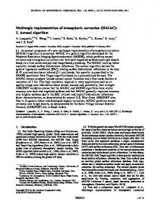
external file names, and some graphical representation of the results: figures showing receiver positions, satellite availabilities over time, the time series of I2+ corrections applied. More details about the service can be found online. 3 Experimental campaigns In order to validate the impact of I2+ corrections on precise GNSS applications, we have selected three test periods with different ionosphere activity characteristics over Poland. We processed GNSS data from stations distributed worldwide, as well. In addition, we selected two regional networks: in Poland (representing mid-latitude region) and Brazil (representing low-latitude region) for positioning and troposphere estimation tests. The midlatitude region is characterized by the most stable ionosphere conditions, while the low latitudes are characterized by the highest TEC level [Bergeot et al., 2013], where we expect the highest influence of the I2+ effects. 3.1 Selection of test periods The three test periods, one week long each were as follows (Figure 1): 

SMAXc – October 24-30, Day of Year (DoY) 297-303, 2014 (Poland and Brazil);



GSTOc – March 14-20, DoY 73-79, 2015 (Poland);



SMINc – September 12-18, DoY 254-260, 2015 (Poland).

The SMAXc period was characterized by a high TEC level, with the maximum VTEC value up to 28 TECu and 260 TECu for Poland and Brazil, respectively. The disturbance storm time index Dst did not fall below -10 nT. The GSTOc period represents the disturbed ionosphere conditions, with a main phase of ionosphere storm on March 17, 2015. Three first days of the GSTOc period were characterized by the sum of 8 planetary indices for the day ƩKp=19, Dst ranging 0 to 25 nT and VTEC below 30 TECu (Poland). During the fourth day the ƩKp reached 48, Dst dropped down to - 225nT and VTEC exceeded 40 TECu. Then, during the next three days the maximum ƩKp amounted to 39, Dst was increasing to -50 nT and VTEC was below 18 TECu. These characteristics allows us to classify this period as a typical storm event with an initial phase (March 14-16), a main ionosphere storm phase (March 17) and a recovery phase (March 18-20) according to Adeniyi [1986] and Joshua et al., [2014]. The SMINc period is characterized by low VTEC, not exceeding 15 TECu during daytime. The Dst has not fallen below -50 nT indicating regular geomagnetic conditions.


Figure 1. Ionospheric conditions during test periods (Poland)

3.2 GNSS networks We used data from the following GNSS networks: IGS, ASG-EUPOS in Poland, SmartNet Poland, and the Brazilian Network for Continuous Monitoring of the GNSS Systems (RBMC). The data from the RBMC network were only available for the SMAXc period. GNSS data for the Polish network were available for all three periods, with some exceptions for new and modernized stations, which were missing in 2014, e.g. KUTN, LODZ, RWM1, as well as for station SKIE in 2015 which was inactive during two selected test periods. The average inter-station distances are 64 km and 94 km in Poland and Brazil, respectively. 60 selected IGS stations were used in a global solution to estimate orbits and clocks of GPS and GLONASS satellites. Troposphere parameters were estimated for selected IGS stations, for 21 selected RBMC stations, for all ASG-EUPOS and SmartNet stations. To evaluate I2+ impact on real-time kinematics (RTK) and PPP, we used 6 stations from Brazil and 7 stations from Poland.


Figure 2. Location of GNSS test stations

4 Results We evaluated results of the STEC calibration and characteristics of I2+ corrections for selected stations over three test periods. We compared solutions obtained in two processing variants: 1) without I2+ corrections and 2) with I2+ corrections, in order to evaluate the impact of I2+ corrections on troposphere estimates, long-range RTK, orbit and clock estimation, static and kinematic PPP. In variant 2), the I2+ corrections were applied in advance in the RINEX file. 4.1 Higher-order ionospheric corrections In order to compute four higher order ionospheric terms, in the first step, a geometryfree linear combination of dual-frequency carrier-phase observations is calculated. Then, the ionospheric delay calculated by using VTEC provided by UQRG GIMs and the geometryfree linear combination are used to calibrate a constant carrier phase bias in continuous-phase arcs. The computation of calibrated STEC is done by fitting carrier phase geometry-free linear combination into GIM. In this way, GIMs bias is reduced and resulting (calibrated) STEC is of the highest quality. For 7 selected stations in Poland, during all three test periods, I2+ analysis were performed. During the SMAXc period characterized by high TEC level reflecting solar max conditions, the ionospheric I2+ corrections varied from -13 mm to +2 mm and from -26 mm to +5 mm for L1 and L2 signals, respectively. For the GSTOc period, covering disturbed ionosphere conditions, during three magnetically quiet days before the storm (14-16 March), I2+ ionospheric corrections for L1 signal varied from -12 mm to +2 mm, while the I2+ corrections for L2 signal reached between -24 mm and +3 mm. During the main phase of the storm (17 March), the I2+ correction values for L1 increased up to -15 mm, and the I2+ corrections values for L2 signal varied from -26 mm to +4 mm. This level of corrections corresponded to dynamic STEC variations with TEC values up to 180 TECU. The recovery phase of the storm was characterized by a low level of TEC, which in turn resulted in low values of I2+ corrections. These effects fell from -7 mm to +1, and from -15 mm to +2 mm for L1 and L2 signals, respectively. For the SMINc period, the I2+ionospheric corrections varied from -6 mm to +1 mm for L1 signal, with the most negative values occurring also


during noontime, which reflected changes at STEC level. Regarding L2 signal, the I2+ corrections were two times larger when compared to L1 signals, reaching from -12 mm to +2 mm. This came from the signal frequencies that were in the 3rd power in case of the second order effects (see Equation 4). Figure 3 provides examples of the ionospheric I2+ corrections and separate impacts of the second- and third-order terms, as well as geometric bending and differential STEC bending effects on the total I2+ corrections. In this example, during all three test periods for WAT1 station, the I2 effects for L1 signal are the greatest, and during SMAXc period vary form -11 mm to +2 mm, while the I3 term values change from -1.4 mm to 0 mm. The impact of both the geometric bending and differential STEC bending effects on the I2+ corrections is very small, clearly below 1 mm. These effects can be seen also for the other test weeks. In general, the I2 effect constitutes up to 90% of the total I2+ delay. Note that for the second GPS frequency the I2+ effect is roughly higher by 50%. The selected stations of the Brazilian network were analyzed only during the SMAXc period. The maximum STEC daily level reached 300 TECU during noontime for low elevation satellites. These STEC values were almost two times higher than the corresponding STEC values during the time over Polish stations. During the SMAXc period, I2+ corrections values were similar. The I2+ corrections for L1 signal varied from -10 mm to +11 mm, while the I2+ corrections for L2 signal reached from -24 mm up to +23 mm.

Figure 3. I2+ corrections for L1 carrier-phase observations for station WAT1 (Poland); top plot presents the I2+ corrections in total, other plots show the contribution of each term

4.2 Estimation of orbits and clocks We estimated GPS+GLONASS orbits, clock corrections and Earth Rotation Parameters (ERPs: X and Y pole offsets, UT1-UTC corrections) with and without I2+


corrections of GNSS observations from 60 globally distributed IGS stations (Figure 2). The average number of stations during each processed day was 56. In total, 36 stations out of the selected 60 tracked both GPS and GLONASS satellites. Satellite orbits and clocks were estimated for all periods additionally including one day before and after each period, in order to estimate the final products in three day windows. The processing was done in Bernese GNSS Software v.5.2 [Dach et al., 2015] following the strategy developed by the Center for Orbit Determination in Europe (CODE) [Dach et al., 2017]. The processing was based on the different ambiguity resolution (AR) strategies for different baseline lengths. Daily normal equations were solved in long-arc 3-day windows to increase the accuracy of the estimated orbits and ERPs, following the method described by Lutz et al. [2016]. Obtained orbits and ERPs corresponded to the middle day of a 3-day window in case of a long-arc analysis. Highrate (30 s interval) satellite clock corrections were estimated using PPP approach without fixed phase ambiguities. We investigated the internal solution quality by means of the following parameters: 1) a posteriori error of unit weight, 2) the consistency of overlaps of solutions and 3) formal errors of estimated parameters. A posteriori error of unit weight was calculated from residuals of the least squares solution of normal equations [Dach et al., 2015]. Consistency of overlaps was evaluated using RMS of differences between parameters estimated in consecutive solutions (last day of a 3-day window compared with a middle day of the following solution). Formal errors were taken directly from the variance-covariance matrix resulting from the least-square solution. One exception here is the calculation of the orbit quality, where the RMS errors of estimated orbital elements (semi major axis, eccentricity, inclination, ascending node, perigee, argument of latitude) and dynamic parameters (direct solar radiation pressure, bias in the line of satellite’s solar panel axis, acceleration perpendicular to the two other terms) carry no direct geometric error meaning. Therefore, we compared estimated orbits to a priori orbits from CODE final GPS+GLONASS solutions [Dach et al., 2017].

Figure 4. Mean quality of estimated GPS and GLONASS orbits obtained with I2+ corrections

There were no differences in the a posteriori error of unit weight between processing variants, which was expected, due to the processing of the same baseline sets. We also found that adding I2+ introduces no significant improvement in the consistency of overlaps. Mean RMS of overlaps was 19.9 mm, while the differences between variants with and without I2+ corrections were below 0.1 mm. Formal errors of estimated parameters were within the range from 1.3 mm to 1.4 mm in all periods, thus indicating a good quality of solutions. The comparison with a priori orbits (Figure 4) in the radial, along-track and cross-track components showed a better mean quality of GPS orbits (21 mm of the mean satellite position RMS) than that of GLONASS (42 mm). The quality of estimated GPS orbits was similar to IGS final solution (RMS=2.5 mm), while the quality of estimated GLONASS orbits is slightly degraded compared to IGS final product (RMS=30 mm). The worse quality of GLONASS orbits can be explained by a smaller number of GLONASS tracking stations, and a poor quality of the cross-track component for R11 and R12 which was already identified by Prange et al. [2017] © 2017 American Geophysical Union. All rights reserved.

The a posteriori errors of unit weight obtained from PPP clock estimations were within the range of 0.83 – 1.05 mm. There were no significant differences between the a posteriori errors of unit weight calculated with or without I2+ corrections. Moreover, no significant differences were found in mean daily formal errors of satellite clock correction estimates, which varied from 24 mm to 30 mm for GPS and from 27 mm to 35 mm for GLONASS. Formal errors obtained the largest values during the SMAXc period, reflecting the high activity of the ionosphere. The average quality of the obtained clock correction was slightly worse than the quality of the IGS final clocks, with the formal error of 75 ps, which corresponds to 23 mm. The degradation of clock quality can be explained by a relatively small global network used in our study, as opposed to the higher number of stations used by IGS analysis centers, e.g. the CODE final clock solution employs 270 stations [Dach et al., 2017]. Formal errors in solutions with and without I2+ reflected also the same quality of estimated ERPs. The mean formal errors of the X and Y pole offsets varied from 0.013 mas during the GSTOc period to 0.016 mas during the SMINc period. The UT1-UTC correction RMS errors were 0.14 µs for the SMAXc period and 0.13 µs for both the GSTOc and the SMINc periods. Orbits and clock estimated with and without I2+ corrections were compared to each other. For orbits, we investigated differences for the radial, along-track and cross-track component. Clock differences were transformed into metric values by multiplying by the speed of light. We found the differences between products are at the sub-centimeter level (Table 1). We noticed the smallest differences were obtained for the radial component with RMS not exceeding 1.0 mm, while the differences for along-track and cross-track components were relatively larger, with RMS up to 3.8 mm. The orbital differences among all periods were at a similar level, except for the along- and cross-track components, for which the RMS values were larger during the SMAXc period. This was not the case for clock differences, which were the smallest during the SMINc period, with RMS reaching up to 3 mm. For other test periods, the impact of I2+ on clocks was larger, but the RMS of differences was still below 5 mm and 7 mm for the GSTOc and the SMAXc periods, respectively. We have not found any significant differences in performance among systems, satellites or particular days, except for GLONASS satellites R10 and R14 during DoY 78, 2015 (Figure 5). In this case, the differences reached several centimeters for all orbital components and clocks. This can be explained by insufficient GNSS network tracking GLONASS satellites. In order to avoid the impact of these outlying results, we did not use R10 and R14 during DoY 78, 2015 in further processing. Table 1. RMS of differences between GPS and GLONASS orbital components and clocks estimated with and without I2+ corrections SMAXc GSTOc SMINc GPS GLO GPS GLO GPS GLO Radial [mm] 0.9 1.0 0.8 1.0 0.7 0.8 Along-track [mm] 3.8 3.2 2.8 2.8 2.2 2.4 Cross-track [mm] 3.2 3.3 2.5 2.7 2.0 2.1 Clock [mm] 6.2 6.9 4.5 5.0 2.7 3.0


Figure 5. Time series of differences between GPS and GLONASS orbits and clocks estimated with and without I2+ corrections

4.3 Troposphere estimation We estimated zenith total delay (ZTD) and horizontal gradients: GN and GE in North and East direction, respectively, for all test stations (Figure 2) and all three test periods. We applied modified RINEX-to-SINEX strategy based on double-differences of phase GNSS observations, originally distributed with the Bernese GNSS Software v5.2. The strategy is based on the different AR strategies for various baseline lengths. The troposphere delay model applied for GNSS data processing was based on Saastamoinen [1973] formula combined with hydrostatic and non-hydrostatic Global Mapping Functions (GMF) [Boehm et al., 2006], which is one of the strategies used by European Permanent Network processing centers. Slant total delays (STDs) to reduce GNSS observation were calculated as: 𝑆𝑇𝐷 = 𝑍𝐻𝐷𝐺𝑀𝐹 ∗ 𝑚𝑓𝑑𝑟𝑦 ,𝐺𝑀𝐹 + 𝑍𝑊𝐷𝑒𝑠𝑡𝑖𝑚𝑎𝑡𝑒𝑑 ∗ 𝑚𝑓𝑤𝑒𝑡 ,𝐺𝑀𝐹 + 𝑚𝑓𝑔𝑟𝑎𝑑𝑖𝑒𝑛𝑡 𝐺𝑁 ∗ cos 𝜙 + 𝐺𝐸 ∗ sin 𝜙

(11)

where ZHDGMF is a priori zenith hydrostatic delay calculated employing Saastamoinen formula with air pressure and temperature from standard atmosphere model, ZWDestimated is the estimated zenith wet delay, mfdry,GMF and mfwet,GMF are hydrostatic and non-hydrostatic mapping functions from GMF, 𝑚𝑓𝑔𝑟𝑎𝑑𝑖𝑒𝑛𝑡 is ZTD horizontal gradient mapping function, ϕ is the azimuth of the horizontal gradient. ZTDs were estimated with 0.5 hour interval, whereas gradients were estimated once per day. The solution was constrained according to the reference frame realization using the no-net rotation minimum constraint on a subset of stable IGS stations. Troposphere parameters were not absolutely constrained, however, very loosely relative constrained (1 m/hour) both for ZTD and gradients, which means that almost no troposphere constraining was applied which would prevent from estimating outlying troposphere parameters when using incomplete data sets. Table 2. Summary statistics of ZTD and gradient differences (with I2+ minus without I2+) ZTD [mm] GN [mm] GE [mm] Network Period Mean Std.Dev. Mean Std.Dev. Mean Std.Dev.

GLOBAL

SMAXc GSTOc SMINc

-0,127 -0.078 0.000

0.329 0.272 0.146

0.014 0.009 0.008

0.017 0.021 0.007

0.000 0.002 -0.001

0.012 0.012 0.004


SMAXc Poland GSTOc SMINc SMAXc Brazil GSTOc SMINc Total mean Mean for SMAXc all GSTOc networks SMINc

-0.037 -0.025 -0.017 -0.202 -0.057 0.005 -0.060 -0.122 -0.053 -0.004

0.074 0.099 0.068 0.351 0.315 0.117 0.197 0.251 0.229 0.110

0.009 0.008 0.003 0.010 0.012 0.007 0.009 0.011 0.010 0.006

0.003 0.005 0.002 0.016 0.011 0.005 0.010 0.012 0.012 0.005

0.003 -0.001 0.000 -0.008 -0.004 -0.003 -0.001 -0.002 -0.001 -0.001

0.001 0.003 0.003 0.014 0.012 0.005 0.007 0.009 0.009 0.004

Figure 6. Time series of ZTD differences (with I2+ minus without I2+) for stations in Brazil during SMAXc period

Table 2 shows that the I2+ corrections to GNSS data caused limited effects. On average ZTD were underestimated by -0.06 mm, the North gradients were overestimated by up to 0.01mm and almost no change was noticed for the East gradients. Extreme ZTD differences were obtained for the station CORD in Brazil during the SMAXc period (3.4 mm) and for station JAGA in Poland during the SMINc period (-4.4 mm). Extreme differences for the North gradient were obtained for PIMO station in Brazil (0.320 mm) and station TAH1 in Tahiti on Pacific (-0.466 mm), both during the GSTOc period. Maximum values of differences for the East gradient were obtained for the Polish station JAGA during the SMINc period (0.297 mm) and the station MCIL in Japan in the Pacific during the GSTOc period (0.152 mm). ZTD difference results obtained for near-equatorial areas in Brazil presented the oscillatory trend, which may be caused by the improvement in ionosphere effect reduction by the introduction of I2+ corrections. The largest magnitude of ZTD difference oscillations was in the SMAXc period (Figure 6), moderate in the GSTOc period and the lowest in the SMINc. Most of the differences of mean troposphere parameter results were statistically insignificant, because differences were smaller than their standard deviations (Table 2). The largest difference was obtained during the SMAXc period. The mean impact of I2+ corrections on ZTD is -0.06 mm, with the standard deviation of 0.197 mm. The mean impact on horizontal gradients is 0.009 mm and -0.001 mm with 0.010 and 0.007 mm of standard deviation for 𝐺𝑁 and 𝐺𝐸 , respectively. These numbers correspond with the results presented by Petrie et al. [2010] and Hernández-Pajares et al. [2014].


4.4 Long-range RTK positioning The impact of I2+ corrections on wide range RTK was investigated by means of AR performance, in the coordinate domain and in the observation domain. In Poland, we used station LOWI as a rover receiver, and stations KUTN, PLON and RWMZ as reference stations. In Brazil, reference stations were MGIN, POLI and SPPI, while SPCA was used as a rover receiver. RTK positioning was performed using GINPOS - in-house developed software [Paziewski, 2015]. One of the most effective and well-recognized models for wide range GNSS RTK positioning, applicable for baselines of dozens of kilometers and more, is the so-called ionosphere-weighted model which takes into account ionospheric delay parametrization [Bock et al., 2000, Odijk, 2001, Paziewski, 2016, Paziewski and Wielgosz, 2017]. Thus, our applied functional model takes into account the influence of the ionospheric delay, which is commonly related to first order ionospheric corrections derived from the reference network solution. In the regular solution I2+ delays are neglected, however, this study aims at analysis of the influence of I2+ corrections and related products. The summary of processing strategy for RTK positioning is given in Table 3. Observables

Table 3. Summary of the RTK processing strategy Double-differenced L1/L2 GPS phase and code

A priori Std.Dev. of observations

0.3 m for raw code, 0.002 m for raw phase

Observables weighting

Elevation-dependent weighting

Elevation cut-off angle

10°

Sampling rate

Poland: 30 s, Brazil 15 s

Single session duration

Poland: 10 min (20 epochs), 144 sessions per day; Brazil: 30 min (120 epochs), 48 sessions per day

First order ionosphere delay

derived from reference network solution

Higher order ionosphere delay

RINEX with or without I2+ corrected observations

Troposphere delay modeling

Fixed ZTD estimated with consistent I2+ modelling + GMF

Satellite orbits and clocks

Estimated from global network, with consistent I2+ modelling

Solution type

Multi-station kinematic with AR (MLAMBDA) and validation (W-ratio)

We begin with a brief analysis of the indicators of AR performance and AR reliability obtained in the experiment in Poland. As the indicators the reliability of the AR, we adopted the average Time-To-first-ambiguity-Fix (TTF) defined as a number of epochs required to obtain correct position solution within set threshold of coordinate residuals, and the percentage of epochs with passed ambiguity validation process with W-ratio >3.0 evaluated. In the Polish network experiment, the percentage of epochs with W-ratio passing the adopted threshold was relatively high reaching up to 98%. For the majority of the days during the SMINc period this indicator was above 94%. This shows a high performance and reliability of the AR process. During high activity of the ionosphere this indicator has dropped, however, no substantial differences between the two processing variants were noticed (Table 4). Generally the results obtained in the Brazil network were experienced by lower values of the W-ratio in relation to study based on the Polish network during the corresponding test period. This indicates a lower reliability of AR in Brazil, which may be caused by the higher influence of the atmospheric delays and high effectiveness of their elimination. In Brazil during the SMAXc period the percentage of epochs passing W-ratio


threshold was in the range between 36.4% - 53.4% depending on the day. However, for the analyzed indicator no significant differences between variants could be seen (Table 4). The difference between daily mean TTF obtained for processing variants did not exceed 0.2 epochs for particular days, with similar values of weekly averages (Table 4). Generally the impact of the I2+ corrections on the performance and reliability of AR in RTK can be considered as limited for such lengths of baselines, i.e., up to 100 km. Table 4. Mean % for each period ratio of epochs with passed ambiguity validation process (W-ratio >3.0) and mean for each Time-To-Fix [epochs] SMAXc GSTOc SMINc Region without I2+ with I2+ without I2+ with I2+ without I2+ with I2+ Poland 76.4 76.4 83.4 83.8 94.9 94.8 Epochs with W-ratio >3.0 Brazil 46.1 46.1 2.1 2.1 2.2 2.2 1.5 1.5 Mean Time-To- Poland Fix Brazil 18.1 18.4 -

According to coordinate domain results, we observe insignificant differences (