December 6th, 2013, ppOpen-HPC and Automatic Tuning (Chair: Hideyuki Jitsumoto), 1330-1400 ... Keeping high performance in multiple computer.
Impact of Auto-tuning of Kernel Loop Transformation by using ppOpen-AT Takahiro Katagiri Supercomputing Research Division, Information Technology Center, The University of Tokyo Collaborators: Satoshi Ohshima, Masaharu Matsumoto (Information Technology Center, The University of Tokyo)
.
SPNS2013, December 5th -6th, 2013 Conference Room, 3F, Bldg.1, Earthquake Research Institute (ERI), The University of Tokyo December 6th, 2013, ppOpen-HPC and Automatic Tuning (Chair: Hideyuki Jitsumoto), 1330-1400
1
Outline Background ppOpen-AT
System Target Application and Its Kernel Loop Transformation Performance Evaluation Conclusion 2
Outline Background ppOpen-AT
System Target Application and Its Kernel Loop Transformation Performance Evaluation Conclusion 3
Performance Portability (PP)
Keeping high performance in multiple computer environments. ◦ Not only multiple CPUs, but also multiple compilers. ◦ Run-time information, such as loop length and number of threads, is important. Auto-tuning (AT) is one of candidate technologies to establish PP in multiple computer environments.
4
Software Architecture of ppOpen-HPC User’s Program ppOpen-APPL
ppOpen-MATH
FEM
FDM
MG
GRAPH
STATIC
ppOpen-AT
FVM
BEM
VIS
DEM
MP
DYNAMIC Auto-Tuning Facility
Code Generation for Optimization Candidates Search for the best candidate Automatic Execution for the optimization
ppOpen-SYS
COMM
Specify The Best Execution Allocations
FT Resource Allocation Facility
Many-core CPUs
GPU
Low Power CPUs
Vector CPUs 5
Outline Background ppOpen-AT
System Target Application and Its Kernel Loop Transformation Performance Evaluation Conclusion 6
Design Policy of ppOpen-AT Domain Specific Language (DSL) for Dedicated Processes for ppOpen-HPC Simple functions of languages to restrict computation patterns in ppOpen-HPC. II. Directive-base AT Language Codes of ppOpen-HPC are frequently modified, since it is under development software. To add AT functions, we provide AT by a directive-base manner. I.
7
Design Policy of ppOpen-AT (Cont’d) III.
IV.
Utilizing Developer’s Knowledge Some loop transformations require increase of memory and/or computational complexities. To establish the loop transformation, user admits via the directive. Minimum Software-Stack Requirement To establish AT in supercomputers in operation, our AT system does not use dynamic code generator. No daemon and no dynamic job submission are required. No script language is also required for the AT system. 8
ppOpen‐AT System Library Developer
Before User ① ppOpen‐APPL /* Release‐time Knowledge Automatic ppOpen‐AT Code Directives ② Generation ppOpen‐APPL / *
Selection
ppOpen‐AT Auto‐Tuner ⑤
Auto‐tuned Kernel ⑥ Execution Library User
③
Library Call
④
Candidate Candidaten
3 Candidate 2 Candidate 1
Execution Time :Target Computers
Run‐ time
A Scenario to Software Developers for
ppOpen-AT Software Developer Description of AT by Using
ppOpen-AT
Invocate dedicated Preprocessor Program with AT Functions Executable Code with Optimization Candidates and AT Function
Description By Software Developer Optimizations for Source Codes, Computer Resource, Power Consumption #pragma oat install unroll (i,j,k) region start #pragma oat varied (i,j,k) from 1 to 8
for(i = 0 ; i < n ; i++){ for(j = 0 ; j < n ; j++){ for(k = 0 ; k < n ; k++){ A[i][j]=A[i][j]+B[i][k]*C[k][j]; }}} #pragma oat install unroll (i,j,k) region end
■Automatic Generated Functions Optimization Candidates Performance Monitor Parameter Search Performance Modeling
Optimization that cannot be established by compilers 10
Power Optimization for Science and Technology Computations
Algorithm selection function on ppOpen‐AT. Automatic selection for implementation to minimize energy between CPU and GPU executions according to problem sizes. Addition to AT function of ppOpen‐AT, technology for power measurement and AT numerical infrastructures is used. This is a joint work with Suda Lab., U.Tokyo. [IEEE MCSoC‐13]
ppOpen‐AT Description (C Language) #pragma OAT call OAT_BPset("nstep") #pragma OAT install select region start #pragma OAT name SelectPhase #pragma OAT debug (pp) #pragma OAT select sub region start at_target(mgn, nx, ny, n, dx, dy, delta, nstep, nout, 0, calc_coef_a_w_pmobi, init, model); #pragma OAT select sub region end #pragma OAT select sub region start at_target(mgn, nx, ny, n, dx, dy, delta, nstep, nout, 1, calc_coef_a_w_pmobi, init, model); #pragma OAT select sub region end #pragma OAT install select region end
Automatic Generation Target Codes API for power measuring CPU Execution GPU Execution AT Numerical Infrastructures
P_initial(); P_start(); P_stop(); P_recv(&rec); P_close();
Power Auto‐tuner
Optimizing Energy by measuring powers
Target Program + AT Auto‐tuner
Target Computer PSU: •12V power line PCI-Express bus:
Current probes p
•12V power line •3.3V power line
volatge p probes
GPU power GPU card
12V
PSU
C P U
3.3V
Main Board
PCIExpress
12V
Outline • Background • ppOpen‐AT System • Target Application and Its Kernel Loop Transformation • Performance Evaluation • Conclusion 12
Target Application Seism_3D: Simulation for seismic wave analysis.
Developed by Professor Furumura at the University of Tokyo. ◦ The code is re-constructed as ppOpen-APPL/FDM.
Finite Differential Method (FDM) 3D simulation ◦ 3D arrays are allocated. Data type: Single Precision (real*4)
13
The Heaviest Loop(10%~20% to Total Time) DO K = 1, NZ DO J = 1, NY DO I = 1, NX RL = LAM (I,J,K) RM = RIG (I,J,K) RM2 = RM + RM RLTHETA = (DXVX(I,J,K)+DYVY(I,J,K)+DZVZ(I,J,K))*RL QG = ABSX(I)*ABSY(J)*ABSZ(K)*Q(I,J,K) SXX (I,J,K) = ( SXX (I,J,K)+ (RLTHETA + RM2*DXVX(I,J,K))*DT )*QG SYY (I,J,K) = ( SYY (I,J,K)+ (RLTHETA + RM2*DYVY(I,J,K))*DT )*QG Flow Dependency SZZ (I,J,K) = ( SZZ (I,J,K) + (RLTHETA + RM2*DZVZ(I,J,K))*DT )*QG RMAXY = 4.0/(1.0/RIG(I,J,K) + 1.0/RIG(I+1,J,K) + 1.0/RIG(I,J+1,K) + 1.0/RIG(I+1,J+1,K)) RMAXZ = 4.0/(1.0/RIG(I,J,K) + 1.0/RIG(I+1,J,K) + 1.0/RIG(I,J,K+1) + 1.0/RIG(I+1,J,K+1)) RMAYZ = 4.0/(1.0/RIG(I,J,K) + 1.0/RIG(I,J+1,K) + 1.0/RIG(I,J,K+1) + 1.0/RIG(I,J+1,K+1)) SXY (I,J,K) = ( SXY (I,J,K) + (RMAXY*(DXVY(I,J,K)+DYVX(I,J,K)))*DT) * QG SXZ (I,J,K) = ( SXZ (I,J,K) + (RMAXZ*(DXVZ(I,J,K)+DZVX(I,J,K)))*DT) * QG SYZ (I,J,K) = ( SYZ (I,J,K) + (RMAYZ*(DYVZ(I,J,K)+DZVY(I,J,K)))*DT) * QG END DO END DO END DO 14
Loop fusion – One dimensional (a loop collapse) Merit: M it Loop L length l th is i hhuge. This is good for OpenMP thread parallelism and GPU.
DO KK = 1, NZ * NY * NX K = (KK-1)/(NY*NX) + 1 J = mod((KK-1)/NX,NY) + 1 I = mod(KK-1,NX) + 1 RL = LAM (I,J,K) RM = RIG (I,J,K) RM2 = RM + RM RMAXY = 4.0/(1.0/RIG(I,J,K) + 1.0/RIG(I+1,J,K) + 1.0/RIG(I,J+1,K) + 1.0/RIG(I+1,J+1,K)) RMAXZ = 4.0/(1.0/RIG(I,J,K) + 1.0/RIG(I+1,J,K) + 1.0/RIG(I,J,K+1) + 1.0/RIG(I+1,J,K+1)) RMAYZ = 4.0/(1.0/RIG(I,J,K) + 1.0/RIG(I,J+1,K) + 1.0/RIG(I,J,K+1) + 1.0/RIG(I,J+1,K+1)) RLTHETA = (DXVX(I,J,K)+DYVY(I,J,K)+DZVZ(I,J,K))*RL QG = ABSX(I)*ABSY(J)*ABSZ(K)*Q(I,J,K) SXX (I,J,K) = ( SXX (I,J,K) + (RLTHETA + RM2*DXVX(I,J,K))*DT )*QG SYY (I,J,K) = ( SYY (I,J,K) + (RLTHETA + RM2*DYVY(I,J,K))*DT )*QG SZZ (I,J,K) = ( SZZ (I,J,K) + (RLTHETA + RM2*DZVZ(I,J,K))*DT )*QG SXY (I,J,K) = ( SXY (I,J,K) + (RMAXY*(DXVY(I,J,K)+DYVX(I,J,K)))*DT )*QG SXZ (I,J,K) = ( SXZ (I,J,K) + (RMAXZ*(DXVZ(I,J,K)+DZVX(I,J,K)))*DT )*QG SYZ (I,J,K) = ( SYZ (I,J,K) + (RMAYZ*(DYVZ(I,J,K)+DZVY(I,J,K)))*DT )*QG END DO 15
Loop fusion – Two dimensional
Example:
Merit: Loop length is huge. DO KK = 1, NZ * NY K = (KK-1)/NY + 1 This is good for OpenMP thread parallelism and GPU. J = mod(KK-1,NY) + 1 DO I = 1, NX This I-loop enables us an opportunity of pre-fetching RL = LAM (I,J,K) RM = RIG (I,J,K) RM2 = RM + RM RMAXY = 4.0/(1.0/RIG(I,J,K) + 1.0/RIG(I+1,J,K) + 1.0/RIG(I,J+1,K) + 1.0/RIG(I+1,J+1,K)) RMAXZ = 4.0/(1.0/RIG(I,J,K) + 1.0/RIG(I+1,J,K) + 1.0/RIG(I,J,K+1) + 1.0/RIG(I+1,J,K+1)) RMAYZ = 4.0/(1.0/RIG(I,J,K) + 1.0/RIG(I,J+1,K) + 1.0/RIG(I,J,K+1) + 1.0/RIG(I,J+1,K+1)) RLTHETA = (DXVX(I,J,K)+DYVY(I,J,K)+DZVZ(I,J,K))*RL QG = ABSX(I)*ABSY(J)*ABSZ(K)*Q(I,J,K) SXX (I,J,K) = ( SXX (I,J,K) + (RLTHETA + RM2*DXVX(I,J,K))*DT )*QG SYY (I,J,K) = ( SYY (I,J,K) + (RLTHETA + RM2*DYVY(I,J,K))*DT )*QG SZZ (I,J,K) = ( SZZ (I,J,K) + (RLTHETA + RM2*DZVZ(I,J,K))*DT )*QG SXY (I,J,K) = ( SXY (I,J,K) + (RMAXY*(DXVY(I,J,K)+DYVX(I,J,K)))*DT )*QG SXZ (I,J,K) = ( SXZ (I,J,K) + (RMAXZ*(DXVZ(I,J,K)+DZVX(I,J,K)))*DT )*QG SYZ (I,J,K) = ( SYZ (I,J,K) + (RMAYZ*(DYVZ(I,J,K)+DZVY(I,J,K)))*DT )*QG ENDDO END DO 16
Loop Split with Re-Computation DO K = 1, NZ DO J = 1, NY DO I = 1, NX RL = LAM (I,J,K) RM = RIG (I,J,K) RM2 = RM + RM RLTHETA = (DXVX(I,J,K)+DYVY(I,J,K)+DZVZ(I,J,K))*RL QG = ABSX(I)*ABSY(J)*ABSZ(K)*Q(I,J,K) SXX (I,J,K) = ( SXX (I,J,K) + (RLTHETA + RM2*DXVX(I,J,K))*DT )*QG SYY (I,J,K) = ( SYY (I,J,K) + (RLTHETA + RM2*DYVY(I,J,K))*DT )*QG SZZ (I,J,K) = ( SZZ (I,J,K) + (RLTHETA + RM2*DZVZ(I,J,K))*DT )*QG ENDDO DO I = 1, NX STMP1 = 1.0/RIG(I,J,K) STMP2 = 1.0/RIG(I+1,J,K) STMP4 = 1.0/RIG(I,J,K+1) STMP3 = STMP1 + STMP2 RMAXY = 4.0/(STMP3 + 1.0/RIG(I,J+1,K) + 1.0/RIG(I+1,J+1,K)) RMAXZ = 4.0/(STMP3 + STMP4 + 1.0/RIG(I+1,J,K+1)) RMAYZ = 4.0/(STMP3 + STMP4 + 1.0/RIG(I,J+1,K+1)) QG = ABSX(I)*ABSY(J)*ABSZ(K)*Q(I,J,K) SXY (I,J,K) = ( SXY (I,J,K) + (RMAXY*(DXVY(I,J,K)+DYVX(I,J,K)))*DT )*QG SXZ (I,J,K) = ( SXZ (I,J,K) + (RMAXZ*(DXVZ(I,J,K)+DZVX(I,J,K)))*DT )*QG SYZ (I,J,K) = ( SYZ (I,J,K) + (RMAYZ*(DYVZ(I,J,K)+DZVY(I,J,K)))*DT )*QG END DO END DO END DO
Re-computation is needed. ⇒Compilers do not apply it without directive.
17
Perfect Split: Two 3-nested Loops DO K = 1, NZ DO J = 1, NY DO I = 1, NX RL = LAM (I,J,K) RM = RIG (I,J,K) RM2 = RM + RM RLTHETA = (DXVX(I,J,K)+DYVY(I,J,K)+DZVZ(I,J,K))*RL QG = ABSX(I)*ABSY(J)*ABSZ(K)*Q(I,J,K) SXX (I,J,K) = ( SXX (I,J,K) + (RLTHETA + RM2*DXVX(I,J,K))*DT )*QG SYY (I,J,K) = ( SYY (I,J,K) + (RLTHETA + RM2*DYVY(I,J,K))*DT )*QG SZZ (I,J,K) = ( SZZ (I,J,K) + (RLTHETA + RM2*DZVZ(I,J,K))*DT )*QG ENDDO; ENDDO; ENDDO
Perfect Splitting
DO K = 1, NZ DO J = 1, NY DO I = 1, NX STMP1 = 1.0/RIG(I,J,K) STMP2 = 1.0/RIG(I+1,J,K) STMP4 = 1.0/RIG(I,J,K+1) STMP3 = STMP1 + STMP2 RMAXY = 4.0/(STMP3 + 1.0/RIG(I,J+1,K) + 1.0/RIG(I+1,J+1,K)) RMAXZ = 4.0/(STMP3 + STMP4 + 1.0/RIG(I+1,J,K+1)) RMAYZ = 4.0/(STMP3 + STMP4 + 1.0/RIG(I,J+1,K+1)) QG = ABSX(I)*ABSY(J)*ABSZ(K)*Q(I,J,K) SXY (I,J,K) = ( SXY (I,J,K) + (RMAXY*(DXVY(I,J,K)+DYVX(I,J,K)))*DT )*QG SXZ (I,J,K) = ( SXZ (I,J,K) + (RMAXZ*(DXVZ(I,J,K)+DZVX(I,J,K)))*DT )*QG SYZ (I,J,K) = ( SYZ (I,J,K) + (RMAYZ*(DYVZ(I,J,K)+DZVY(I,J,K)))*DT )*QG END DO; END DO; END DO;
18
New ppOpen-AT Directives - Loop Split & Fusion with data-flow dependence !oat$ install LoopFusionSplit region start !$omp parallel do private(k,j,i,STMP1,STMP2,STMP3,STMP4,RL,RM,RM2,RMAXY,RMAXZ,RMAYZ,RLTHETA,QG) DO K = 1, NZ DO J = 1, NY DO I = 1, NX RL = LAM (I,J,K); RM = RIG (I,J,K); RM2 = RM + RM RLTHETA = (DXVX(I,J,K)+DYVY(I,J,K)+DZVZ(I,J,K))*RL !oat$ SplitPointCopyDef region start QG = ABSX(I)*ABSY(J)*ABSZ(K)*Q(I,J,K) !oat$ SplitPointCopyDef region end SXX (I,J,K) = ( SXX (I,J,K) + (RLTHETA + RM2*DXVX(I,J,K))*DT )*QG SYY (I,J,K) = ( SYY (I,J,K) + (RLTHETA + RM2*DYVY(I,J,K))*DT )*QG SZZ (I,J,K) = ( SZZ (I,J,K) + (RLTHETA + RM2*DZVZ(I,J,K))*DT )*QG !oat$ SplitPoint (K, J, I) STMP1 = 1.0/RIG(I,J,K); STMP2 = 1.0/RIG(I+1,J,K); STMP4 = 1.0/RIG(I,J,K+1) STMP3 = STMP1 + STMP2 RMAXY = 4.0/(STMP3 + 1.0/RIG(I,J+1,K) + 1.0/RIG(I+1,J+1,K)) RMAXZ = 4.0/(STMP3 + STMP4 + 1.0/RIG(I+1,J,K+1)) RMAYZ = 4.0/(STMP3 + STMP4 + 1.0/RIG(I,J+1,K+1)) !oat$ SplitPointCopyInsert SXY (I,J,K) = ( SXY (I,J,K) + (RMAXY*(DXVY(I,J,K)+DYVX(I,J,K)))*DT )*QG SXZ (I,J,K) = ( SXZ (I,J,K) + (RMAXZ*(DXVZ(I,J,K)+DZVX(I,J,K)))*DT )*QG SYZ (I,J,K) = ( SYZ (I,J,K) + (RMAYZ*(DYVZ(I,J,K)+DZVY(I,J,K)))*DT )*QG END DO; END DO; END DO !$omp end parallel do !oat$ install LoopFusionSplit region end
Re-calculation is defined in here.
Loop Split Point
Using the re-calculation is defined in here.
19
Automatic Generated Codes for the kernel 1 ppohFDM_update_stress
#1 [Baseline]: Original 3-nested Loop #2 [Split]: Loop Splitting with K-loop (Separated, two 3-nested loops) #3 [Split]: Loop Splitting with J-loop #4 [Split]: Loop Splitting with I-loop #5 [Split&Fusion]: Loop Fusion to #1 for K and J-loops (2-nested loop) #6 [Split&Fusion]: Loop Fusion to #2 for K and J-Loops (2-nested loop) #7 [Fusion]: Loop Fusion to #1 (loop collapse) #8 [Split&Fusion]: Loop Fusion to #2 (loop collapse, two one-nest loop)
Outline • Background • ppOpen‐AT System • Target Application and Its Kernel Loop Transformation • Performance Evaluation • Conclusion 21
An Example of Seism_3D Simulation
West part earthquake in Tottori prefecture in Japan at year 2000. ([1], pp.14) The region of 820km x 410km x 128 km is discretized with 0.4km. NX x NY x NZ = 2050 x 1025 x 320 ≒ 6.4 : 3.2 : 1.
Figure : Seismic wave translations in west part earthquake in Tottori prefecture in Japan. (a) Measured waves; (b) Simulation results; (Reference : [1] in pp.13) [1] T. Furumura, “Large-scale Parallel FDM Simulation for Seismic Waves and Strong Shaking”, Supercomputing News, Information Technology Center, The University of Tokyo, Vol.11, Special Edition 1, 2009. In Japanese.
Problem Sizes (Tottori Prefecture Earthquake) 8 Nodes(8MPI Processes, Minimum running condition of ppOpen‐APPL/FDM with respect to 32GB/node) Value of NZ
Problem Sizes (NX x NY x NZ)
Process Grid (Pure MPI, the FX10)
Problem Size per Core
Weak Scaling, Problem Sizes when we use whole nodes of the FX10 (65,536 Cores、 Pure MPI Process Grid: 64 x 64 x 16)
10
64 x 32 x 10
8 x 8 x 2
8 x 4 x 5
512 x 256 x 80
128 x 64 x 20
8 x 8 x 2
16 x 8 x 10
1024 x 512 x 160
256 x 128 x 40
8 x 8 x 2
32 x 16 x 20
2048 x 1024 x 320
80
512 x 256 x 80
8 x 8 x 2
64 x 32 x 40
4096 x 2048 x 640
160
1024 x 512 x 160
8 x 8 x 2
128 x 64 x 80
8192 x 4096 x 1280
20 40
Same as size as Tottori’s Earthquake Simulation
320 2048 x 1024 x 320 8 x 8 x 2 (Maximum Size for 32GB /node)
256 x 128 x 160 16384 x 8192 x 2560
AT Effect for Hybrid OpenMP‐MPI PXTY :X Processes, Y Threads / Process
Original without AT Speedup to pure MPI Execution
1
The FX10, Kernel: update_stress With AT(Speedups to the case without AT) 2.5
No merit for Hybrid MPI‐OpenMPI Executions.
1 Effect on pure MPI Execution Gain by using MPI‐OpenMPI Executions.
Pure MPI
Types of hybrid MPI‐OpenMP Execution
Pure MPI
Types of hybrid MPI‐OpenMP Execution
By adapting loop transformation from the AT, we obtained: Maximum 1.5x speedup to pure MPI (without Thread execution) Maximum 2.5x speedup to pure MPI in hybrid MPI‐OpenMP execution.
OTHER KERNEL AND CODE OPTIMIZATION
Kernel update_vel (ppOpen‐APPL/FDM) • m_velocity.f90(ppohFDM_update_vel) !OAT$ install LoopFusion region start !OAT$ name ppohFDMupdate_vel !OAT$ debug (pp) !$omp parallel do private(k,j,i,ROX,ROY,ROZ) do k = NZ00, NZ01 do j = NY00, NY01 do i = NX00, NX01 !OAT$ RotationOrder sub region start ROX = 2.0_PN/( DEN(I,J,K) + DEN(I+1,J,K) ) ROY = 2.0_PN/( DEN(I,J,K) + DEN(I,J+1,K) ) ROZ = 2.0_PN/( DEN(I,J,K) + DEN(I,J,K+1) ) !OAT$ RotationOrder sub region end !OAT$ RotationOrder sub region start VX(I,J,K) = VX(I,J,K) + ( DXSXX(I,J,K)+DYSXY(I,J,K)+DZSXZ(I,J,K) )*ROX*DT VY(I,J,K) = VY(I,J,K) + ( DXSXY(I,J,K)+DYSYY(I,J,K)+DZSYZ(I,J,K) )*ROY*DT VZ(I,J,K) = VZ(I,J,K) + ( DXSXZ(I,J,K)+DYSYZ(I,J,K)+DZSZZ(I,J,K) )*ROZ*DT !OAT$ RotationOrder sub region end end do; end do; end do !$omp end parallel do !OAT$ install LoopFusion region end
Reorder of sentences !OAT$ RotationOrder sub region start Sentence i Sentence ii !OAT$ RotationOrder sub region end Sentences 1 !OAT$ RotationOrder sub region start Sentence I Sentence II !OAT$ RotationOrder sub region end
Automatic Code Generation Sentence 1 Sentence i Sentence I Sentence ii Sentence II
AT Effect for Hybrid OpenMP‐MPI ●Intel Sandy Bridge, NZ=320 (Maximum Size by Memory Restriction) Speedups 1.021 1.02 1.02
Kernel: update_stress
1.019 1.018 1.017
Upper is better.
1.017
1.016 1.015 Speedups 3.8
P16T1 3.75
3.7
Kernel: update_vel
3.6
P8T2
Loop Fusion for k, j‐loops + re‐ordering
3.75x
3.57
P16T1
P8T2
3.5 3.4
AT Effect for Hybrid OpenMP‐MPI ●Intel Xeon Phi, NZ=80 (Maximum Size by Memory Restriction) Speedups 2000
Kernel: update_stress
Loop Split By J‐loop
1500 1000 500 60.5
121
1563
844
1563x
P16T15
P8T30
240
0 P240T1 P120T2 Speedups 40
Kernel: update_vel
P60T4
Loop Fusion for k, j‐loops + re‐ordering
30 20 10 0
1.03 P240T1
2.37
4.76
P120T2
P60T4
29.8
15.3
29.8x
P16T15
P8T30
Related Work (AT Languages) AT Language / Items ppOpen‐AT Vendor Compilers Transformation Recipes POET X language SPL
# 1 OAT Directives Out of Target Recipe Descriptions Xform Description Xlang Pragmas SPL Expressions ADAPT Language
# 2 ✔
# 3 ✔
# 4 ✔
# 5 ✔
# 7 None
Limited ✔
✔
✔
✔
✔
✔
✔ ✔
✔
ADAPT
Atune‐IL
# 6
atune Pragmas
#1: Method for supporting multi-computer environments.
✔
✔ ✔
‐ ChiLL POET translator, ROSE X Translation, ‘C and tcc A Script Language Polaris Compiler Infrastructure, Remote Procedure Call (RPC) A Monitoring Daemon
#2: Obtaining loop length in run-time.
#3: Loop split with increase of computations, and loop fusion to the split loop. #4: Re-ordering of inner-loop sentences. #6: Code generation with execution feedback.
#5: Algorithm selection. #7: Software requirement.
Outline • Background • ppOpen‐AT System • Target Application and Its Kernel Loop Transformation • Performance Evaluation • Conclusion 31
Conclusion Kernel
loop transformation is a key technology to establish high performance for current multi-core and many-core processors. Utilizing run-time information for problem sizes (loop length) and the number of threads is important. Minimum software stack for auto-tuning facility is required for supercomputers in operation.
32
ppOpen-AT is free software! ppOpen-AT
version 0.2 is now available! The licensing is MIT. Or, please access the following page: http://ppopenhpc.cc.u-tokyo.ac.jp/
33