Implementation of a Time-Domain Random-Walk Method into a ...

Hindawi Geofluids Volume 2017, Article ID 5940380, 13 pages https://doi.org/10.1155/2017/5940380

Research Article Implementation of a Time-Domain Random-Walk Method into a Discrete Element Method to Simulate Nuclide Transport in Fractured Rock Masses Yuexiu Wu,1 Quansheng Liu,1 Andrew H. C. Chan,2 and Hongyuan Liu2 1

Key Laboratory of Rock Mechanics in Hydraulic Structural Engineering, Ministry of Education, Wuhan University, Wuhan, Hubei 430072, China 2 School of Engineering and ICT, University of Tasmania, Hobart, TAS 7005, Australia Correspondence should be addressed to Yuexiu Wu; [email protected] Received 12 May 2017; Accepted 20 June 2017; Published 15 August 2017 Academic Editor: Paolo Fulignati Copyright © 2017 Yuexiu Wu et al. This is an open access article distributed under the Creative Commons Attribution License, which permits unrestricted use, distribution, and reproduction in any medium, provided the original work is properly cited. It is essential to study nuclide transport with underground water in fractured rock masses in order to evaluate potential radionuclide leakage in nuclear waste disposal. A time-domain random-walk (TDRW) method was firstly implemented into a discrete element method (DEM), that is, UDEC, in this paper to address the pressing challenges of modelling the nuclide transport in fractured rock masses such as massive fractures and coupled hydromechanical effect. The implementation was then validated against analytical solutions for nuclide transport in a single fracture and a simple fracture network. After that, the proposed implementation was applied to model the nuclide transport in a complex fracture network investigated in the DECOVALEX 2011 project to analyze the effect of matrix diffusion and stress on the nuclide transport in the fractured rock masses. It was concluded that the implementation of the TDRW method into UDEC provided a valuable tool to study the nuclide transport in the fractured rock masses. Moreover, it was found that the total travel time of the nuclide particles in the fractured rock masses with the matrix diffusion and external stress modelled was much longer than that without the matrix diffusion and external stress modelled.

1. Introduction 1.1. Significance. With the development of nuclear waste disposal, nuclide transport with underground water in fractured rock masses has been an important issue in recent decades [1]. Especially after the nuclear leakage accident in Fukushima in Japan [2], this becomes more and more pressing. Therefore, it is essential to understand the principal transport mechanisms of radionuclides with underground water in fractured rock masses and evaluate the potential of radionuclide leakage from the repositories to the biosphere. 1.2. Literature Review about Nuclide Transport Simulation. Once the radionuclide is released from the container, it will flow with underground water in fractured rock masses to the biosphere. Therefore, water flow process in fractured rock masses should be studied firstly and foremost. Till now, five models have been found in literatures to simulate the water

flow in fractured rock masses, that is, continuous model [3–5], dual-continuum model [6–8], equivalent continuum model [9–11], discrete fracture network (DFN) [12–14], and hybrid model [15–17]. In continuous model, rock masses are treated as continuum porous media with porosity and permeability and continuum-mechanics formulations can be used to describe flow and transport in media. It is a simple way but does not reflect the real flow path and velocity distribution in rock masses. In dual-continuum model, the rock matrix and fractures are represented as two overlapping and interactive continuum media with different mechanical and flow characteristics. However, this model cannot be applied to disconnected fractures in fractured media and the evaluation of fluid exchange between the matrix and the fractured domain is a complex task. In equivalent continuum model, fractured rock masses are treated as equivalent continua for large-scale analyses with equivalent mechanical and hydraulic properties that are measured or calculated in

2 Representative Element Volume (REV). Nevertheless, REV may not exist for fractured rock masses in general. Moreover, flow rate in fractures is much larger than that in rock matrix. Thus, the DFN seems to be more suitable to simulate the water flow in fractured rock masses, irrespective of its high demand of computer resource. As a matter of fact, DFN has already been implemented into several numerical methods to simulate water flow in fractured rock masses, such as distinct deformation analysis (DDA) [18, 18–22], numerical manifold method (NMM) [23, 24], extended finite element method (XFEM) [25–27], and discrete element method (DEM) [28, 29]. Compared with other numerical methods, DEM coupled with DFN shows the advantages of simulating water flow through fractured rock masses, since it is capable of simulating coupled hydromechanical effect and, especially, massive fractures. Secondly, radionuclide transport process associated with water flow through fractured rock masses should be analyzed. According to former researches [30, 31], the difficulty of discovering nuclide transport mechanism lies in solving the partial differential transport equation. As mentioned by Delay et al. [32], Lagrangian schemes (particle tracking methods) are more accurate and less computationally intensive than Eulerian schemes. The main Lagrangian schemes include random-walk particle tracking (RWPT) method [33, 34], convolution-based particle tracking (CBPT) method [35, 36], and continuous-time random-walk (CTRW) method [37, 38]. For very heterogeneous media such as fractured rock mass, flow velocities may span several orders of magnitude. With the RWPT method, a large number of jumps are required in low-velocity areas to move the particles significantly, which may cause the calculations to become inefficient in terms of computational costs. The CBPT method is valid for mainly steady-state flow field and linear transport process. Some discrepancies are caused when the CTRW method is employed to the advection-dispersion equation. Aiming at removing these constraints, Delay and Bodin [39] firstly proposed a new method called time-domain random-walk (TDRW) method to simulate solute transport in heterogeneous media, which was further extended to simulate solute transport in fractured rock masses [40–42]. As can be seen from the literature review above, DEM and the TDRW method have the advantages of modelling water flow and solute transport in fractured rock masses. Thus, the TDRW method was firstly implemented into the DEM software UDEC in this paper. 1.3. Objectives and Organization of Paper. The primary objective of this paper is to propose a new numerical tool to simulate nuclide transport with underground water in fractured rock mass. In order to achieve this objective, the paper is organized as follows. Theoretical introduction about hydromechanical coupling in UDEC is given in Section 2; Section 3 discusses nuclide transport equation and theory about time-domain random-walk method; the implementation of TDRW into UDEC is given in Section 4; verification of implementation program with analytical solution is given in Section 5; Section 6 discusses application of implementation program

Geofluids to DECOVALEX (DEmonstration of COupled models and their VALidation against EXperiment) 2011 project to analyze the effect of matrix diffusion and stress on nuclide transport process; and conclusion is given in Section 7. Throughout this study, it was concluded that, due to the effects of both matrix diffusion and stress, it took much more time for particles to outflow the fractured rock masses. Moreover, the proposed numerical method is a valuable numerical tool to study nuclide transport process through fractured rock masses, which has also wide applications in the field of underground water pollution, oil reservoir engineering, and so on.

2. Principle of Flow in UDEC In UDEC [43], fractured rock masses are divided into many deformable blocks whose boundaries are fractures. Each deformable block is meshed into triangle elements, as shown in Figure 1. Motion is first calculated at the grid points of triangle elements within blocks and the stresses within the elements are then obtained according to the block material constitutive relations. Moreover, a fully coupled mechanicalhydraulic analysis can also be performed in UDEC, in which matrix is regarded as impermeable and fluid flows only through fractures. 2.1. Mechanical Behavior. For any grid point 𝑝 in a triangle element, the total force is obtained as a sum of four terms: 𝐹𝑝 = 𝐹𝑝𝑧 + 𝐹𝑝𝑐 + 𝐹𝑝𝑜 + 𝐹𝑝𝑔 ,

(1)

where 𝐹𝑝𝑜 are the external applied loads, 𝐹𝑝𝑧 are the internal stresses contributed by zones adjacent to grid point 𝑝, 𝐹𝑝𝑐 𝑔 are the contact forces from all the adjacent blocks, and 𝐹𝑝 are gravity forces. The internal stress is calculated using the following equation: 𝐹𝑝𝑧 = ∫ 𝜎𝑖𝑗 𝑛𝑗 𝑑𝑠, 𝐶

(2)

where 𝜎𝑖𝑗 is element stress tensor and 𝑛𝑗 is the unit vector outward normal to the integral path 𝐶, which follows the closed polygonal line around the grid point 𝑝. The gravity force is calculated using the following equation: 𝐹𝑝𝑔 = 𝑔𝑝 𝑚𝑝 ,

(3)

where 𝑚𝑝 is the lumped gravitational mass, defined as the sum of one-third of the masses of triangles connected to the grid point, and 𝑔𝑝 is the gravitational acceleration. The contact force 𝐹𝑝𝑐 exists only when grid points are on block boundaries (like grid point 𝑛 in Figure 1) and is calculated according to the contact type and joint constitutive model. Taking the Coulomb slide model as an example, the contact force at the grid point from an adjacent block is divided into two components: 𝐹𝑝nc (normal contact force) and 𝐹𝑝sc (shear contact force): 𝐹𝑝nc fl 𝐹𝑝nc − 𝑘𝑛 Δ𝑢𝑛 𝑙,

(4)

Geofluids

3 Block i1

Grid point m

Grid point n

Block j1

Block k1

Figure 1: Deformable blocks.

where Δ𝑢𝑛 is the normal displacement increment for each contact, 𝑘𝑛 is joint normal stiffness, and 𝑙 is the contact area, and 𝐹𝑝sc fl 𝐹𝑝sc − 𝑘𝑠 Δ𝑢𝑠 𝑙,

(5)

where Δ𝑢𝑠 is the shear displacement increment and 𝑘𝑠 is joint shear stiffness. If the shear contact force exceeds the shear strength, it is modified according to the following equation: 𝐹𝑝sc = sign (Δ𝑢𝑠 ) (𝑐 + tan 0) ,

(6)

where 𝑐 is joint cohesion and 0 is joint frictional strength. The motion of the grid point is obtained according to Newton’s second law: 𝑑𝑢̇𝑝 𝑑𝑡

=

𝐹𝑝 𝑚𝑝

,

(7)

where 𝑢̇𝑝 is the velocity of grid point 𝑝 and 𝑡 is time. After the calculation of displacement of each grid point, the strain and stress of each triangle element are obtained according to the block constitutive model: Δ𝜀𝑖𝑗 =

1 (𝑢 + 𝑢𝑗,𝑖 ) Δ𝑡, 2 𝑖,𝑗

(8)

where Δ𝑡 is time step. Δ𝜎𝑖𝑗 = 𝜆Δ𝜀V 𝛿𝑖𝑗 + 2𝜇Δ𝜀𝑖𝑗 ,

differently. For a point contact (from a domain with pressure 𝑝1 to a domain with pressure 𝑝2 ), 𝑞 = −𝑘𝑐 Δ𝑝,

where 𝑞 is the flow rate, 𝑘𝑐 is a point contact permeability factor, and Δ𝑝 is the pressure difference calculated using the following equation: Δ𝑝 = 𝑝2 − 𝑝1 + 𝜌𝑤 𝑔 (𝑦2 − 𝑦1 ) ,

where 𝜆 and 𝜇 are Lame’s constant and Δ𝜀V is the bulk strain. 2.2. Fluid Flow in Fractures. Depending on the different contact type, the flow rate in contact domain is calculated

(11)

where 𝜌𝑤 is the fluid density; 𝑔 is the acceleration of gravity; and 𝑦2 and 𝑦1 are 𝑦-coordinates of the domain centers which are perpendicular to the joint surface. For edge-edge contact (an edge of one element contacts with an edge of another element), the flow rate in contact domain is calculated using the following equation: 𝑞 = −𝑘𝑗 𝑎3

Δ𝑝 , 𝑙

(12)

where 𝑘𝑗 is a joint permeability factor (whose theoretical value is one-twelfth dynamic viscosity of fluid), 𝑎 is the contact hydraulic aperture, and 𝑙 is the length assigned to the contact between the domains. Fluid velocity can be obtained using (13) according to the flow rate calculated according to (10) and (12): 𝑢𝑓 =

(9)

(10)

𝑞 , 𝐴

(13)

where 𝐴 is the fluid crossing area. 2.3. Coupled Mechanical-Hydraulic Analysis. When the fluid flows in the contact domain, the fluid pressure is regarded as an external force applied on the contact domain, which

4

Geofluids

2b

y

Matrix

Matrix

Stagnant zone

Research zone

Matrix

Matrix

Matrix x

Stagnant zone Matrix

Figure 2: Fracture with an aperture of 2𝑏.

is added into 𝐹𝑝𝑜 . The external force is calculated using the following equation: 𝐹𝑝𝑃 = 𝑝𝑛𝑖 𝐿,

The retardation factor 𝑅𝑓 is defined using the following equation [42]:

(14)

𝑅𝑓 = 1 +

𝐾𝑓 𝑏

,

(17)

where 𝑝 is the fluid pressure in a contact domain, 𝑛𝑖 is the normal direct of contact, and 𝐿 is the contact length. With the motion of each block, the contact area will change following (15), which causes flow rate variation:

where 𝐾𝑓 is the surface sorption coefficient of nuclide onto the fracture surface. The nuclide transport equation in rock matrix can be written as follows [42]:

𝑎 = 𝑎0 + Δ𝑢𝑛 ,

𝜕2 𝑐 𝜕𝑐𝑚 , + 𝜆𝑐𝑚 = 𝐷𝑎 𝑚 𝜕𝑡 𝜕𝑦2

(15)

where 𝑎0 is the initial fracture aperture and Δ𝑢𝑛 is the normal displacement of contact area.

3. Nuclide Transport 3.1. Nuclide Transport Equation. It is known that nuclide transport is the consequence of several physical mechanisms such as advection, hydrodynamic dispersion, matrix diffusion, decay, and adsorption. As mentioned by Bodin et al. [42], the nuclide transport can be described in three media: (1) fracture, (2) matrix, and (3) stagnant zone. The stagnant zones in the fracture plane act as an additional “nonflowing” pore space available for solute diffusion. Thus, transport in the stagnant zone is ignored in this study. The nuclide transport equation in 2D fracture can be written as follows [42]: 𝜕𝑐𝑓 𝜕𝑡

+ 𝜆𝑐𝑓 = −

𝑢𝑓 𝜕𝑐𝑓 𝑅𝑓 𝜕𝑥

+

𝜕𝑐𝑓 1 𝜕 (𝐷𝑓 ) 𝑅𝑓 𝜕𝑥 𝜕𝑥

𝐷𝑓 𝜕𝑐𝑚 󵄨󵄨󵄨 󵄨󵄨 , + 𝑏𝑅𝑓 𝜕𝑦 󵄨󵄨󵄨𝑦=𝑏

where 𝐷𝑎 is the apparent-diffusion coefficient of the nuclide in the matrix, which is calculated as 𝐷𝑎 = 𝐷𝑒 /(𝜃𝑚 + 𝜌𝑚 𝐾𝑚 ); 𝐷𝑒 is effective diffusion coefficient; 𝜃𝑚 is matrix porosity; 𝜌𝑚 is matrix density; and 𝐾𝑚 is volumetric-sorption coefficient of the nuclide in the matrix. 3.2. Time-Domain Random-Walk Method 3.2.1. Advection-Dispersion-Sorption Equation. In TDRW method, the solution of (16) can be divided into three steps: (1) advection-dispersion-sorption (ADS) transport equation, (2) decay effect, and (3) matrix diffusion effect. The ADS equation can be rewritten as (19) [42], considering the change of variable (𝜕𝑐𝑓 /𝜕𝑡 = (𝜕𝑐𝑓 /𝜕𝑥)(𝜕𝑥/𝜕𝑡) = (𝜕𝑐𝑓 /𝜕𝑥)(𝑢𝑓 /𝑅𝑓 )): 𝜕𝑐𝑓 𝜕𝑥

(16)

where 𝑐𝑓 is the concentration of nuclide in fracture, 𝑢𝑓 is the fluid velocity in fracture, 𝑏 is half of the aperture, 𝑐𝑚 is the concentration of nuclide in rock matrix, 𝜆 is the decay constant of nuclide, the term 𝜆𝑐𝑓 represents the decay effect, 𝐷𝑓 is the hydrodynamic dispersion coefficient in fracture, 𝑅𝑓 is a retardation factor accounting for the sorption of nuclide onto fracture surface, the last term on the right of the equation represents the matrix diffusion effect, and 𝑥 and 𝑦 are the space coordinates along and perpendicular to the fracture, respectively, as shown in Figure 2. Not considering the effect of decay and matrix diffusion, the equation becomes the advection-dispersion-sorption (ADS) equation.

(18)

=−

𝑅𝑓2 𝜕2 𝜕𝐷𝑓 𝑅𝑓 𝜕 + ] + (𝐷𝑓 𝑐𝑓 ) . (19) [(𝑢 ) 𝑐 𝑓 𝑓 𝜕𝑥 𝑢𝑓2 𝜕𝑡 𝑢𝑓3 𝜕𝑡2

By applying an equivalent change of variable, (19) can be written with Fokker-Planck formalism: 2 𝜕𝜑 1 𝜕 (V𝜑) 1 𝜕 (0𝜑) . =− 2 + 3 𝜕𝑥 V 𝜕𝑡 2V 𝜕𝑡2

(20)

According to the solution of random-walk approach, the mean and variance of nuclide transport time distribution for a displacement of 𝑑𝑥 are obtained using (21a) and (21b), respectively [42]: 𝜇𝑡 (𝑑𝑥) =

𝑅𝑓 𝑢𝑓2

𝜎𝑡2 (𝑑𝑥) = 𝑅𝑓2

(𝑢𝑓 + 2𝐷𝑓 𝑢𝑓3

𝜕𝐷𝑓

𝑑𝑥.

𝜕𝑥

) 𝑑𝑥,

(21a)

(21b)

Geofluids

5

For Peclet number Pe = 𝑢𝑓 𝑑𝑥/𝐷𝑓 larger than 10, it is shown that the travel time distribution is lognormal for a displacement of 𝑑𝑥 [30]: ln (Δ𝑡𝑓 ) = 𝜇ln + 𝑍𝑁𝜎ln , 𝜇ln = ln (

𝜇𝑡 √1 + 𝜎𝑡2 /𝜇𝑡2

2 𝜎ln = ln (1 +

(22a) ),

(22b)

𝜎𝑡2 ), 𝜇𝑡2

(22c)

where Δ𝑡𝑓 is the travel time of the nuclide for a displacement 𝑑𝑥 and 𝑍𝑁 is a random number that follows a standard normal distribution. For very low flow velocities in short fractures (i.e., the Peclet number Pe is less than 10), the assumption of a lognormal distribution is not accurate. Bodin et al. [30] suggested that (22b) should be modified: 󸀠 = 𝛽𝜇ln = (1 − 𝜇ln

𝜇𝑡 1 ). ) ln ( 33Pe √1 + 𝜎2 /𝜇2 𝑡

(23)

(for Pe > 10) .

(24)

When Peclet number Pe is less than 10, the variable 𝜇ln is 󸀠 . replaced by 𝜇ln 3.2.2. Matrix Diffusion. To account for the interaction between ADS and matrix diffusion in a bond of length 𝑑𝑥, the fluid velocity 𝑢𝑓 and dispersion coefficient 𝐷𝑓 in (22a) and (22b) were replaced by an apparent fluid velocity 𝑢𝑓∗ and an apparent dispersion coefficient 𝐷𝑓∗ [42]: 𝑢𝑓∗ = 𝑅diff 𝑢𝑓 , 𝐷𝑓∗ = 𝑓 (𝑢𝑓∗ ) ,

like 𝐷𝑓∗ = 𝛼𝑢𝑓∗ , or 𝐷𝑓∗ = 𝐷𝑓 ,

(25)

where 𝛼 is a dispersivity constant and 𝑅diff is a retardation factor accounting for matrix diffusion: 𝑅diff = 1 +

2

Δ𝑡𝑓𝑚 = exp (𝜇ln + 𝑍𝑁𝜎ln ) + (

Ω𝑡0 ) , 𝑅𝑓 erfc−1 (𝑈01 )

(27)

where 𝑡0 is the particle residence time in the fracture for pure advection delayed by sorption reactions onto the fracture walls, expressed as 𝑡0 = 𝑅𝑓 (𝑑𝑥/𝑢𝑓 ) and 𝑈01 is a random number drawn from a uniform distribution between 0 and 󸀠 . 1. For Pe < 10, the variable 𝜇ln in (27) is replaced by 𝜇ln 3.2.3. Decay Effect. If the linear decay model is used, the nuclide mass decreases according to the following equation [42]: 𝑝

𝑚𝑛+1 = 𝑚𝑛𝑝 exp (−𝜆 (𝑡𝑛+1 − 𝑡𝑛 )) ,

(28)

𝑝

where 𝑚𝑛+1 and 𝑚𝑛𝑝 represent the masses of the nuclide at node 𝑛 + 1 and 𝑛, respectively. For simplicity, the decay effect is not considered here, which accords with the situation in DECOVALEX 2011 project.

𝑡

The total travel time in a fracture of length 𝑑𝑥 can be written as Δ𝑡𝑓 = exp (𝜇ln + 𝑍𝑁𝜎ln )

coupled ADS and matrix diffusion is calculated using (27) for Pe > 10 [42]:

2 Ω√2𝜎𝑡 exp (−𝜉 ) ( − 𝜉) , √𝜋 erfc (𝜉) 𝑅𝑓

(26)

where 𝜉 = (Ω𝑑𝑥/𝑢𝑓 )(√2/𝜎𝑡 ), Ω = √(𝜃𝑚 + 𝜌𝑚 𝐾𝑚 )𝐷𝑒 /2𝑏, 𝜃𝑚 is the matrix porosity, 𝜌𝑚 is the bulk density of matrix, 𝐾𝑚 is the volumetric-sorption coefficient of nuclide in matrix, and 𝐷𝑒 is the effective diffusion coefficient of nuclide in matrix. The modified (22a) and (22b) with 𝑢𝑓∗ and 𝐷𝑓∗ in place of 𝑢𝑓 and 𝐷𝑓 , respectively, were used to calculate the mean and 󸀠 2 ) and 𝜎ln according variance of the log transform 𝜇ln (or 𝜇ln to (22b) and (22c), respectively. The total travel time for the

3.2.4. Mass Partition Model at Fracture Intersection. Because the nuclide was tracked in fractures from the inflow boundary to the outflow boundary in TDRW method, the mass partition model at fracture intersection is vital in the calculation. There are three models: the perfect-mixing model [44], the stream-tube model [45], and the diffusional-mixing model [46]. The focus of this paper is not the mass partition law of solute at fracture intersection. For simplicity, the perfectmixing model was adopted here: 𝑃𝑖𝑗 =

𝑄𝑗 ∑ 𝑄−

,

(29)

where 𝑃𝑖𝑗 is the probability of particle transition from an inlet bond 𝑖 to an outlet bond 𝑗; 𝑄𝑗 is the flow rate in the outlet bond 𝑗; and ∑ 𝑄− is the sum of the flow rates over all the outlet bonds connected to the junction of interest. It can be seen from (29) that mass partition is only related to the outlet fluxes.

4. Implementation of TDRW into UDEC In TDRW method, the fractures are regarded as the sum of many bonds and a continuous connection of the bonds from inlet to outlet boundaries is considered as a flow path (e.g., the dashed line shown in Figure 3). In a bond, the fluid flow is a 1D flow with a constant fluid velocity. Therefore, the first thing, before we do the particle tracking calculation, is to get the flow paths of particle transport. In UDEC, jointed rock masses are divided into blocks by fractures. The geometric information of fracture and block, such as corner coordinates and their connection, is stored in list in files (e.g., BLOCK.FIN, DOMAIN.FIN, and CONTACT.FIN). According to the above files, the coordinates of

6

Geofluids A farther point

All nuclides

Bo nd 1

Inlet boundary

A child point

Bo nd 2

Choose one nuclide

According to the flow rate in each inlet point, the nuclide chooses one as its initial transport location

Bo nd

3

4 nd Bo

The initial farther point is the fracture intersection on inlet boundary

Bon d5

Find the child points connected with the farther point

Each farther point roop

Outlet boundary Fracture intersection Fracture network Flow path

Figure 3: Flow path in fracture network.

fracture intersections can be obtained easily, as well as their connective information. The TDRW method is implemented into UDEC using the FISH language, as shown in Figure 4. After the hydromechanical calculation with UDEC, the final flow velocity at each fracture intersection can be obtained and this is the input data for TDRW simulation. At the beginning, nuclide particles are injected into the fractured rock masses through the inlet boundary. According to the inlet flow rate, the injection location of each particle is chosen. The particle transport time in each bond is calculated with ((22a), (22b), (22c))–(28). At the fracture intersection, the perfect-mixing model is adopted to decide the next step of particles until they arrive at the outlet boundary. If the injected mass is 𝑀0 and the total number of particles is 𝑁, mass of each particle is expressed as 𝑀 𝑚𝑝𝑖 = 0 . 𝑁

𝑚𝑝𝑖 𝑁𝑖 , ∑ 𝑄out 𝑑𝑡

Identify the next transport location by comparing the random number with the transport probability of each child point Regard this child point as a new farther point and calculate the transport time with equation (28) in this bond between farther point and the chosen child point

No

If this child point is on the outlet boundary Yes Another particle

End

Figure 4: Flow chart of TDRW method’s implementation.

(30)

If the collected particle number on the outlet boundary is 𝑁𝑖 in a period of time 𝑑𝑡, the outlet concentration is written as 𝑐𝑖 =

Generate a random number

Each particle roop

Calculate the transport probabilities of child points with equation (30)

(31)

where ∑ 𝑄out is the total outlet fluid flow rate. The following steps are adopted to obtain the curve of the relative concentration versus time: (1) Calculate the maximum and minimum travel times of all particles.

(2) Divide the travel time period (from minimum travel time to maximum travel time) into 𝑁 parts, in which the time interval is Δ𝑡. (3) Collect particles (number is 𝑁𝑖 ) in each time interval and calculate their concentration with (31).

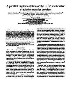
5. Verification Two numerical particle transport tests were performed to verify the implementation of the TDRW method into UDEC,

Geofluids

7

1.0

c/c0

0.8 0.6 0.4 0.2 0.0

0

2

4

6

8

10

Time (×104 Ｍ)

Figure 6: A simple fracture network.

Numerical solution with TDRW Analytical solution

Figure 5: Comparison between numerical and analytical solutions for nuclide particle transport in a single fracture.

1.0

5.1. Analytical Solution of the Nuclide Transport Equation. Analytical solution for nuclide transport in a single fracture has been deduced in literatures [47–49]. The analytical solution is to be used later to verify the numerical results obtained with combination of DEM and TDRW. For simplicity, the analytical solution for advection-dispersion transport equation with constant concentration injection is adopted, which can be written as follows: 𝑐𝑓 𝑐0

=

𝑥 − 𝑢𝑓 𝑡 1[ ) [erfc ( 2 2√𝐷𝑓 𝑡 [

− exp (

𝑢𝑓 𝑥 𝐷𝑓

) erfc (

𝑥 + 𝑢𝑓 𝑡 2√𝐷𝑓 𝑡

c/c0

0.8

that is, particle transports in a single fracture and in a simple facture network.

0.6 0.4 0.2 0.0 0.0

2.0

4.0

6.0

8.0

10.0

12.0

14.0

Time (×107 Ｍ) Numerical results with TDRW Analytical results

Figure 7: Comparison between numerical and analytical solutions of particle transport in a simple fracture network.

(32) ] )] , ]

where 𝑐0 is the constant concentration injection; and erfc(𝑥) is a complementary error function. 5.2. Calibration Test 1: Particle Transport in a Single Fracture. In the calibration test 1 of particle transport in a single fracture, the injection mass at the inlet boundary of the fracture was 0.001 g, and the total number of nuclide particles was 30000. The trace of the fracture was 10 m, fluid velocity was 4.0 × 10−4 m/s, hydrodynamic dispersion coefficient in the fracture was 2.0 × 10−5 m2 /s, and the aperture of the fracture was 2.5 × 10−4 m. Thus, the Peclet number (Pe = 𝑢𝑓 𝐿/𝐷𝑓 ) was 200. The analytical solution can be obtained using (32). The corresponding numerical solution was obtained using the TDRW method implemented into UDEC, which is compared in Figure 5 with the analytical solution. From Figure 5, the maximum and minimum differences between numerical and analytical solutions are 11% and 0.03%, respectively.

The reason for this difference is that the numerical results are iterated. In general, the results from UDEC with the TDRW method implemented agreed well with the analytical solution. 5.3. Calibration Test 2: Particle Transport in a Simple Fracture Network. The simple fracture network was shown in Figure 6. A hydromechanical calculation was performed with UDEC at first. The water heads at top and bottom boundaries were 100 m and 99 m, respectively, and two lateral sides were impermeable. The aperture of the fractures was 2.5 × 10−6 m. The other parameters were the same as those in test 1. The analytical solution was the summarizing solution of (32) for each fracture. Figure 7 was the comparison between the numerical solution and analytical solution for the particle transport in this simple fracture network. From Figure 7, the maximum and minimum differences between numerical and analytical solutions are 10.1% and 0, respectively. From the comparisons shown in Figures 5 and 7, it is concluded that the numerical solution obtained using the

8

Geofluids (10, 10)

Table 1: Material parameters of the fracture in the calculation model.

y

Fractures (0, 0)

x

(−10, −10)

Figure 8: Calculation model studied in the DECOVALEX 2011 project.

TDRW method implemented into UDEC was close to the analytical solution. Thus, it is proven that the TDRW method implemented into UDEC can well simulate nuclide particle transport in fracture networks.

6. Application to Particle Transport in Discrete Fracture Network 6.1. Calculation Models and Material. The proposed method was used to evaluate the effect of matrix diffusion and stress ratio on particle transport process in the fracture network studied in the DECOVALEX 2011 project. The calculation model was shown in Figure 8, which contained 771 fractures. The hydromechanical boundary condition was depicted in Figure 9. The hydraulic heads at the top and bottom boundaries were 30 m and 10 m, respectively. On the two lateral sides, a linear distribution of hydraulic head was applied with a maximum value of 30 m and a minimum value of 10 m; in order to analyze the effect of matrix diffusion, the same hydromechanical boundaries were applied for the case with matrix diffusion and the case without matrix diffusion. Accounting for the effect of stress ratio, simulations without stress (𝜎V = 𝜎ℎ = 0) and with different stress ratios were performed. For the cases with stress, a constant vertical stress of 5 MPa was specified on the top and bottom boundaries. And a horizontal stress, with ratios of vertical/horizontal stress varying from 1 to 2, 3, and 5, was applied, respectively (𝜎V /𝜎ℎ = 1, 2, 3, 5). For each calculation, 10000 particles were injected at a time along the inflow boundary. At each injected point, which is the intersection of fracture and inflow boundary, the injecting particle number is proportional to the local flow rate. This is equivalent to injecting a constant concentration at the inflow boundary. The block material property was 𝐾 = 54.23 GPa, and 𝐺 = 34.11 GPa. The normal behavior of the fractures in the calculation model was nonlinear, as shown in Figure 10 [28]. Other parameters of the fractures were listed in Table 1 [28]. The aperture of the fractures followed a lognormal distribution

Mechanical properties Shear stiffness, 𝐾𝑠 (GPa/m) Friction angle (∘ ) Dilation angle (∘ ) Cohesion (MPa)

Values 434 24.9 5 0

with a mean value of 65 𝜇m and a second moment of 1.0. The minimum and maximum apertures were 1 𝜇m and 200 𝜇m, respectively. The residual aperture was assumed to be 20% of the initial aperture. The hydrodynamic dispersion coefficient in fractures was 1.0 × 10−5 m2 /s. The hydromechanical calculation was done firstly and the fluid velocity could then be obtained. After that, the TDRW simulation was performed. 6.2. Results and Discussion 6.2.1. Fluid Flow. Flow rates in fractures which intersect the bottom, right, and left outlet boundaries with different applied stress were shown in Figures 11–13. The location in Figures 11–13 was the coordinates of intersections of fractures along the corresponding boundary. On the bottom outlet boundary, the maximum flow rate and average flow rate without stress applied were 1.16 × 10−8 m3 /(s⋅m) and 4.06 × 10−9 m3 /(s⋅m), respectively, which were larger than those with stress applied. From Figure 11, it was shown that the main outlet positions (intersections with flow rate larger than the average flowrate) changed comparing the results not considering stress with results considering stress effect. When the stress was applied, the main outlet positions were same for different stress ratio. However, the maximum and average values of flow rate decreased with the increasing of stress ratio. On the right boundary, the maximum and average values of flow rate in intersections without stress were 8.59 × 10−8 m3 /(s⋅m) and 3.13 × 10−8 m3 /(s⋅m), respectively, which were obviously larger than those considering stress ratio. On the left boundary, the maximum and average values of flow rate in intersections without stress were 5.38 × 10−7 m3 /(s⋅m) and 8.02 × 10−8 m3 /(s⋅m), respectively, and the same effect of stress ratio on fluid flow was observed. This was because the fractures were compressed to be narrow with the increasing of external stress and the fluid flow became smaller. 6.2.2. Nuclide Transport (1) Without Matrix Diffusion. After the nuclide transport calculations with different stress ratio, nuclides which outflow the outlet boundary at a certain time were collected. The ratio of number of leaking nuclides from the outlet boundary to the total number of nuclides was plotted versus traveling time (i.e., breakthrough curve) in Figure 14. From Figure 14, it was shown that the total traveling times with different stress boundaries were 1.97 × 104 s, 2.58 × 104 s, 3.12 × 104 s, 1.95 ×

Geofluids

9 

Inflow boundary 0.3 MPa Left outlet boundary

Right outlet boundary

ℎ

0.1 MPa Bottom outlet boundary

Normal stress (×107 ０；)

Figure 9: Hydromechanical boundary condition. 14 12 10 8 6 4 2 0 0.00

15 10 5 1.00

2.00

3.00

4.00

5.00

0 15

6.00

Normal displacement (×10−5 Ｇ)

10

Figure 10: Relationship between normal displacement and normal stress.

(2) With Matrix Diffusion. In the case with matrix diffusion, the porosity of the matrix 𝜃𝑚 was 0.316%. For simplicity, advection, dispersion, and matrix diffusion were considered in this case, while sorption in the matrix was not allowed (𝐾𝑚 = 0 m3 /kg). The effective diffusion coefficient of the nuclide in the matrix is 1.0 × 10−11 m2 /s. The breakthrough curves with different stress applied considering the effect of matrix diffusion were shown in Figure 15. From Figure 15, it was shown that the total traveling times with different stress boundaries were 3.03 × 107 s, 7.98 × 107 s, 1.086 × 108 s, 8.02 × 108 s, and 8.42 × 108 s, respectively. The mean traveling time for each calculation was 4.88 × 106 s, 1.77 × 107 s, 2.89 × 107 s, 5.2 × 107 s, and 7.7 × 107 s, respectively. Through dividing the total traveling times without stress, the normalized total travel times with stress ratio 1, 2, 3, and 5 are 2.63, 3.58, 26.5, and 27.8. The total and average travel times for all nuclides leaking out from the fractured rock masses increased with the increasing of stress ratio.

Flow rate ×10−9 (Ｇ3 /(s·m))

105 s, and 2.4 × 105 s, respectively. The mean traveling time for each calculation was 3.29 × 103 s, 4.31 × 103 s, 5.21 × 103 s, 1.27 × 104 s, and 2.19 × 104 s, respectively. Through dividing the total traveling times without stress, the normalized total travel times with stress ratio 1, 2, 3, and 5 are 1.3, 1.58, 9.89, and 12.18. The total and average travel times for all nuclides leaking out from the fractured rock masses increased with the increasing of stress ratio. The reason for this phenomenon was that fractures were compressed to be narrow and it was difficult for nuclides to leak.

5 0 15 10 5 0 15 10 5 0 15 10 5 0 −15

−10

No stress Ratio = 1 Ratio = 2

−5

0 Location

5

10

15

Ratio = 3 Ratio = 5

Figure 11: Flow rate distribution of fractures on the bottom outlet boundary.

Comparing the breakthrough curves in Figure 14 with those in Figure 15, it could be seen that the total travel time for all particles outflowing from fractured rock masses without the matrix diffusion was much shorter than that with matrix

Geofluids 100

100

75

75

50

50

25

25

0 100

0 20

75

15

50

10

25

5

0 100

Flow rate ×10−9 (Ｇ3 /(s·m))

Flow rate ×10−9 (Ｇ3 /(s·m))

10

75 50 25 0 100

0 20 15 10 5 0 20

75

15

50

10

25

5

0 100

0 600 500 400 300 200 100 0 −15

75 50 25 0 −10

−5

0

5

10

15

−10

Location No stress Ratio = 1 Ratio = 2

Ratio = 3 Ratio = 5

Figure 12: Flow rate distribution of fractures on the right outlet boundary.

No stress Ratio = 1 Ratio = 2

Although the nuclide transport with underground water in fractured rock masses had been studied for decades by many researchers, the coupled hydromechanical effect and the effect of matrix diffusion and stress were still not discussed systematically. Aiming at solving these problems, the time-domain random-walk (TDRW) method was firstly implemented into the discrete element method (DEM) in this study. During each time step of hydromechanical calculation, hydraulic aperture of each fracture and fluid pressure on fracture surface were calculated according to (15) and (14) to consider the coupled hydromechanical effect. To present the effect of matrix diffusion on nuclide transport, (24) and (27)

0 Location

5

10

15

Ratio = 3 Ratio = 5

Figure 13: Flow rate distribution of fractures on the left outlet boundary.

c/c0

diffusion. Thus, the effect of matrix diffusion on the nuclide particle transport was significant.

7. Conclusion

−5

1.0 0.9 0.8 0.7 0.6 0.5 0.4 0.3 0.2 0.1 0.0 5E + 01

5E + 02

5E + 03

5E + 04

5E + 05

Time (s) No stress Ratio = 1 Ratio = 2

Ratio = 3 Ratio = 5

Figure 14: Breakthrough curve with different stress ratios without matrix diffusion.

Geofluids

11

Acknowledgments

1.0 0.9

This work was supported by the Natural Science Foundation of China (nos. 51679172, 41130742, and 51574180), National Basic Research Program of China (973 Program) (no. 2014CB046904), and China Scholarship Council.

0.8 0.7 c/c0

0.6 0.5 0.4

References

0.3 0.2 0.1 0.0 1E + 04

1E + 05

1E + 06 1E + 07 Time (s)

No stress Ratio = 1 Ratio = 2

1E + 08

1E + 09

Ratio = 3 Ratio = 5

Figure 15: Breakthrough curve with different stress ratios with matrix diffusion.

were adopted to get the breakthrough curves. The implementation was then verified against the analytical solutions for nuclide transport in a single fracture and a single fracture network. After that, the implementation was applied to simulate the nuclide transport in a complex fracture network investigated in the DECOVALEX 2011 project. Finally, the effect of matrix diffusion and stress on nuclide transport was discussed in detail. Throughout this study, the following conclusions were drawn: (1) The implementation of the TDRW method into UDEC could well simulate the nuclide transport with underground water in fractured rock masses. (2) Through the hydromechanical calculation for DECOVALEX 2011, the closure of fractures increased with the increasing of applied stress and it caused decreasing of fluid flow in fractured rock masses. More time was needed for fluid or particle transport through a narrower path. This finally resulted in the fact that the total travel time of the nuclide particles with the external stress applied on the fracture network was longer than that without the applied stress. (3) According to the numerical results for the nuclide transport in the complex fracture network investigated in the DECOVALEX 2011 project, matrix diffusion has a significant effect on the nuclide transport. The travel time of the nuclide particle with the matrix diffusion modelled was much longer than that without the matrix diffusion.

Conflicts of Interest The authors declare that the received funds do not lead to any conflicts of interest regarding the publication of this manuscript.

[1] C.-F. Tsang, I. Neretnieks, and Y. Tsang, “Hydrologic issues associated with nuclear waste repositories,” Water Resources Research, vol. 51, no. 9, pp. 6923–6972, 2015. [2] H. Funabashi, “Why the fukushima nuclear disaster is a manmade calamity,” International Journal of Japanese Sociology, vol. 21, no. 1, pp. 65–75, 2012. [3] F. Cappa and J. Rutqvist, “Modeling of coupled deformation and permeability evolution during fault reactivation induced by deep underground injection of CO2 ,” International Journal of Greenhouse Gas Control, vol. 5, no. 2, pp. 336–346, 2011. [4] J. Rutqvist and O. Stephansson, “The role of hydromechanical coupling in fractured rock engineering,” Hydrogeology Journal, vol. 11, no. 1, pp. 7–40, 2003. [5] G. Lei, P.-C. Dong, Z.-S. Wu et al., “A fractal model for the stress-dependent permeability and relative permeability in tight sandstones,” Journal of Canadian Petroleum Technology, vol. 54, no. 1, pp. 36–48, 2015. [6] Y. Hao, P. Fu, and C. R. Carrigan, “Application of a dualcontinuum model for simulation of fluid flow and heat transfer in fractured geothermal reservoirs,” in Proceedings of the 38th Workshop on Geothermal Reservoir Engineering, vol. SGP-TR198, pp. 462–469, Stanford University, Stanford, Calif, USA, 2013. [7] M. Ahmadpour, M. Siavashi, and M. H. Doranehgard, “Numerical simulation of two-phase flow in fractured porous media using streamline simulation and IMPES methods and comparing results with a commercial software,” Journal of Central South University, vol. 23, no. 10, pp. 2630–2637, 2016. [8] J. Douglas Jr., J. L. Hensley, and T. Arbogast, “A dual-porosity model for waterflooding in naturally fractured reservoirs,” Computer Methods in Applied Mechanics and Engineering, vol. 87, no. 2-3, pp. 157–174, 1991. [9] A. R. Khoei, N. Hosseini, and T. Mohammadnejad, “Numerical modeling of two-phase fluid flow in deformable fractured porous media using the extended finite element method and an equivalent continuum model,” Advances in Water Resources, 2015. [10] S. H. Lee, M. F. Lough, and C. L. Jensen, “Hierarchical modeling of flow in naturally fractured formations with multiple length scales,” Water Resources Research, vol. 37, no. 3, pp. 443–455, 2001. [11] M. Oda, “An equivalent model for coupled stress and fluid flow analysis in jointed rock masse,” Water Resources Research, vol. 22, no. 13, pp. 1845–1856, 1986. [12] J. D. Hyman, S. Karra, N. Makedonska, C. W. Gable, S. L. Painter, and H. S. Viswanathan, “DfnWorks: a discrete fracture network framework for modeling subsurface flow and transport,” Computers and Geosciences, vol. 84, pp. 10–19, 2015. [13] J. Maillot, P. Davy, R. Le Goc, C. Darcel, and J. R. de Dreuzy, “Connectivity, permeability, and channeling in randomly distributed and kinematically defined discrete fracture network models,” Water Resources Research, vol. 52, no. 11, pp. 8526– 8545, 2016.

12 [14] S. Follin, L. Hartley, I. Rh´en et al., “A methodology to constrain the parameters of a hydrogeological discrete fracture network model for sparsely fractured crystalline rock, exemplified by data from the proposed high-level nuclear waste repository site at Forsmark, Sweden,” Hydrogeology Journal, vol. 22, no. 2, pp. 313–331, 2014. [15] M. Hu, J. Rutqvist, and Y. Wang, “A practical model for fluid flow in discrete-fracture porous media by using the numerical manifold method,” Advances in Water Resources, vol. 97, pp. 38– 51, 2016. [16] U. Svensson, M. Ferry, and H.-O. Kuylenstierna, “DarcyTools Version 3.4—Concepts, methods and equations,” Tech. Rep. SKB R-07-38, SvenskK€arnbr€anslehantering AB, Stockholm, Sweden, 2010. [17] S. P. Neuman, “Trends, prospects and challenges in quantifying flow and transport through fractured rocks,” Hydrogeology Journal, vol. 13, no. 1, pp. 124–147, 2005. [18] Y.-Y. Jiao, H.-Q. Zhang, H.-M. Tang, X.-L. Zhang, A. C. Adoko, and H.-N. Tian, “Simulating the process of reservoirimpoundment-induced landslide using the extended DDA method,” Engineering Geology, vol. 182, pp. 37–48, 2014. [19] L. Q. Choo, Z. Zhao, H. Chen, and Q. Tian, “Hydraulic fracturing modeling using the discontinuous deformation analysis (DDA) method,” Computers and Geotechnics, vol. 76, pp. 12–22, 2016. [20] W. E. Morgan and M. M. Aral, “An implicitly coupled hydrogeomechanical model for hydraulic fracture simulation with the discontinuous deformation analysis,” International Journal of Rock Mechanics and Mining Sciences, vol. 73, pp. 82–94, 2015. [21] F. Zheng, Y. Jiao, M. Gardner, and N. Sitar, “A fast direct search algorithm for contact detection of convex polygonal or polyhedral particles,” Computers and Geotechnics, vol. 87, pp. 76–85, 2017. [22] F. Zheng, Y.-Y. Jiao, X.-L. Zhang, F. Tan, L. Wang, and Q. Zhao, “Object-oriented contact detection approach for threedimensional discontinuous deformation analysis based on entrance block theory,” International Journal of Geomechanics, vol. 17, no. 5, 2017. [23] H. Zheng, F. Liu, and C. Li, “Primal mixed solution to unconfined seepage flow in porous media with numerical manifold method,” Applied Mathematical Modelling, vol. 39, no. 2, pp. 794–808, 2015. [24] Y. Wang, M. Hu, Q. Zhou, and J. Rutqvist, “Energy-work-based numerical manifold seepage analysis with an efficient scheme to locate the phreatic surface,” International Journal for Numerical and Analytical Methods in Geomechanics, vol. 38, no. 15, pp. 1633–1650, 2014. [25] S. Salimzadeh and N. Khalili, “Fully coupled XFEM model for flow and deformation in fractured porous media with explicit fracture flow,” International Journal of Geomechanics, vol. 16, no. 4, Article ID 04015091, 2016. [26] T. Mohammadnejad and J. E. Andrade, “Numerical modeling of hydraulic fracture propagation, closure and reopening using XFEM with application to in-situ stress estimation,” International Journal for Numerical and Analytical Methods in Geomechanics, vol. 40, no. 15, pp. 2033–2060, 2016. [27] T. Mohammadnejad and A. R. Khoei, “Hydro-mechanical modeling of cohesive crack propagation in multiphase porous media using the extended finite element method,” International Journal for Numerical and Analytical Methods in Geomechanics, vol. 37, no. 10, pp. 1247–1279, 2013.

Geofluids [28] Z. Zhao, L. Jing, I. Neretnieks, and L. Moreno, “Numerical modeling of stress effects on solute transport in fractured rocks,” Computers and Geotechnics, vol. 38, no. 2, pp. 113–126, 2011. [29] L. Quansheng, W. Yuexiu, and L. Bin, “Discrete element analysis of effect of stress on equivalent permeability of fractured rockmass,” Chinese Journal of Rock Mechanics and Engineering, vol. 30, no. 1, pp. 176–183, 2011 (Chinese). [30] J. Bodin, F. Delay, and G. de Marsily, “Solute transport in a single fracture with negligible matrix permeability: 1. Fundamental mechanisms,” Hydrogeology Journal, vol. 11, no. 4, pp. 418–433, 2003. [31] J. Bodin, F. Delay, and G. de Marsily, “Solute transport in a single fracture with negligible matrix permeability: 2. Mathematical formalism,” Hydrogeology Journal, vol. 11, no. 4, pp. 434–454, 2003. [32] F. Delay, P. Ackerer, and C. Danquigny, “Simulating solute transport in porous or fractured formations using random walk particle tracking: a review,” Vadose Zone Journal, vol. 4, no. 2, pp. 360–379, 2005. [33] E. Stalgorova and T. Babadagli, “Field-scale modeling of tracer injection in naturally fractured reservoirs using the randomwalk particle-tracking simulation,” SPE Journal, vol. 17, no. 2, pp. 580–592, 2012. [34] M. Bechtold, J. Vanderborght, O. Ippisch, and H. Vereecken, “Efficient random walk particle tracking algorithm for advective-dispersive transport in media with discontinuous dispersion coefficients and water contents,” Water Resources Research, vol. 47, no. 10, Article ID W10526, 2011. [35] B. A. Robinson, Z. V. Dash, and G. Srinivasan, “A particle tracking transport method for the simulation of resident and flux-averaged concentration of solute plumes in groundwater models,” Computational Geosciences, vol. 14, no. 4, pp. 779–792, 2010. [36] G. Srinivasan, E. Keating, J. D. Moulton, Z. V. Dash, and B. A. Robinson, “Convolution-based particle tracking method for transient flow,” Computational Geosciences, vol. 16, no. 3, pp. 551–563, 2012. [37] P. K. Kang, T. Le Borgne, M. Dentz, O. Bour, and R. Juanes, “Impact of velocity correlation and distribution on transport in fractured media: field evidence and theoretical model,” Water Resources Research, vol. 51, no. 2, pp. 940–959, 2015. [38] S. Geiger, A. Cortis, and J. T. Birkholzer, “Upscaling solute transport in naturally fractured porous media with the continuous time random walk method,” Water Resources Research, vol. 46, no. 12, Article ID W12530, 2010. [39] F. Delay and J. Bodin, “Time domain random walk method to simulate transport by advection-dispersion and matrix diffusion in fracture networks,” Geophysical Research Letters, vol. 28, no. 21, pp. 4051–4054, 2001. [40] V. Cvetkovic, A. Fiori, and G. Dagan, “Solute transport in aquifers of arbitrary variability: A time-domain random walk formulation,” Water Resources Research, vol. 50, no. 7, pp. 5759– 5773, 2014. [41] J. Bodin, “From analytical solutions of solute transport equations to multidimensional time-domain random walk (TDRW) algorithms,” Water Resources Research, vol. 51, no. 3, pp. 1860– 1871, 2015. [42] J. Bodin, G. Porel, F. Delay, F. Ubertosi, S. Bernard, and J.R. de Dreuzy, “Simulation and analysis of solute transport in 2D fracture/pipe networks: The SOLFRAC program,” Journal of Contaminant Hydrology, vol. 89, no. 1-2, pp. 1–28, 2007.

Geofluids [43] Itasca Consulting Group, UDEC User’s Guide, Itasca Consulting Group, Minneapolis, Minn, USA, 2004. [44] K. R. Bradbury and M. A. Muldoon, “Effects of fracture density and anisotropy on delineation of wellhead-projection areas in fractured-rock aquifers,” Applied Hydrogeology, vol. 2, no. 3, pp. 17–23, 1994. [45] R. Parney and L. Smith, “Fluid velocity and path length in fractured media,” Geophysical Research Letters, vol. 22, no. 11, pp. 1437–1440, 1995. [46] Y.-J. Park and K.-K. Lee, “Analytical solutions for solute transfer characteristics at continuous fracture junctions,” Water Resources Research, vol. 35, no. 5, pp. 1531–1537, 1999. [47] J. P. Sauty, “An analysis of hydrodispersive transfer in aquifers,” Water Resources Research, vol. 16, no. 1, pp. 145–158, 1980. [48] S. R. Yates, “An analytical solution for one-dimensional transport in heterogeneous porous media,” Water Resources Research, vol. 26, no. 10, pp. 2331–2338, 1990. [49] D. H. Tang, E. O. Frind, and E. A. Sudicky, “Contaminant transport in fractured porous media: analytical solution for a single fracture,” Water Resources Research, vol. 17, no. 3, pp. 555– 564, 1981.

13

Journal of

International Journal of

Ecology

Journal of

Geochemistry Hindawi Publishing Corporation http://www.hindawi.com

Mining

The Scientific World Journal

Scientifica Volume 2014

Hindawi Publishing Corporation http://www.hindawi.com

Volume 2014

Hindawi Publishing Corporation http://www.hindawi.com

Volume 2014

Hindawi Publishing Corporation http://www.hindawi.com

Volume 2014

Journal of

Earthquakes Hindawi Publishing Corporation http://www.hindawi.com

Hindawi Publishing Corporation http://www.hindawi.com

Volume 2014

Paleontology Journal Hindawi Publishing Corporation http://www.hindawi.com

Volume 2014

Volume 2014

Journal of

Petroleum Engineering

Submit your manuscripts at https://www.hindawi.com

*HRSK\VLFV International Journal of

Hindawi Publishing Corporation http://www.hindawi.com

Advances in

Volume 2014

Hindawi Publishing Corporation http://www.hindawi.com

Volume 2014

Journal of

Mineralogy

Geological Research Volume 2014

Hindawi Publishing Corporation http://www.hindawi.com

Advances in

Geology

Climatology

International Journal of Hindawi Publishing Corporation http://www.hindawi.com

Advances in

Journal of

Meteorology Hindawi Publishing Corporation http://www.hindawi.com

Hindawi Publishing Corporation http://www.hindawi.com

Volume 2014

Volume 2014

Hindawi Publishing Corporation http://www.hindawi.com

International Journal of

Atmospheric Sciences Hindawi Publishing Corporation http://www.hindawi.com

International Journal of

Oceanography Volume 2014

Volume 2014

Hindawi Publishing Corporation http://www.hindawi.com

Oceanography Volume 2014

$SSOLHG (QYLURQPHQWDO 6RLO6FLHQFH +LQGDZL3XEOLVKLQJ&RUSRUDWLRQ KWWSZZZKLQGDZLFRP

Volume 201

Hindawi Publishing Corporation http://www.hindawi.com

Volume 2014

Journal of Computational Environmental Sciences 9ROXPH

Hindawi Publishing Corporation http://www.hindawi.com

Volume 2014