Implementation of an F-statistic all-sky search for continuous ...

arXiv:1402.4974v3 [gr-qc] 10 Apr 2014

Implementation of an F -statistic all-sky search for continuous gravitational waves in Virgo VSR1 data LIGO Scientific Collaboration and Virgo Collaboration J. Aasi1 , B. P. Abbott1 , R. Abbott1 , T. Abbott2 , M. R. Abernathy1 , T. Accadia3 , F. Acernese4,5 , K. Ackley6 , C. Adams7 , T. Adams8 , P. Addesso5 , R. X. Adhikari1 , C. Affeldt9 , M. Agathos10 , N. Aggarwal11 , O. D. Aguiar12 , A. Ain13 , P. Ajith14 , A. Alemic15 , B. Allen9,16,17 , A. Allocca18,19 , D. Amariutei6 , M. Andersen20 , R. Anderson1 , S. B. Anderson1 , W. G. Anderson16 , K. Arai1 , M. C. Araya1 , C. Arceneaux21 , J. Areeda22 , S. M. Aston7 , P. Astone23 , P. Aufmuth17 , C. Aulbert9 , L. Austin1 , B. E. Aylott24 , S. Babak25 , P. T. Baker26 , G. Ballardin27 , S. W. Ballmer15 , J. C. Barayoga1 , M. Barbet6 , B. C. Barish1 , D. Barker28 , F. Barone4,5 , B. Barr29 , L. Barsotti11 , M. Barsuglia30 , M. A. Barton28 , I. Bartos31 , R. Bassiri20 , A. Basti18,32 , J. C. Batch28 , J. Bauchrowitz9 , Th. S. Bauer10 , B. Behnke25 , M. Bejger33 , M. G. Beker10 , C. Belczynski34 , A. S. Bell29 , C. Bell29 , G. Bergmann9 , D. Bersanetti35,36 , A. Bertolini10 , J. Betzwieser7 , P. T. Beyersdorf37 , I. A. Bilenko38 , G. Billingsley1, J. Birch7 , S. Biscans11 , M. Bitossi18, M. A. Bizouard39 , E. Black1 , J. K. Blackburn1 , L. Blackburn40 , D. Blair41 , S. Bloemen42,10, M. Blom10 , O. Bock9 , T. P. Bodiya11 , M. Boer43 , G. Bogaert43 , C. Bogan9 , C. Bond24 , F. Bondu44 , L. Bonelli18,32, R. Bonnand45 , R. Bork1 , M. Born9 , K. Borkowski46 , V. Boschi18 , Sukanta Bose47,13 , L. Bosi48 , C. Bradaschia18 , P. R. Brady16 , V. B. Braginsky38 , M. Branchesi49,50 , J. E. Brau51 , T. Briant52 , D. O. Bridges7 , A. Brillet43 , M. Brinkmann9 , V. Brisson39 , A. F. Brooks1 , D. A. Brown15 , D. D. Brown24 , F. Br¨ uckner24 , 20 34 S. Buchman , T. Bulik , H. J. Bulten10,53 , A. Buonanno54 , R. Burman41 , D. Buskulic3 , C. Buy30 , L. Cadonati55 , G. Cagnoli45 , J. Calder´ on Bustillo56 , E. Calloni4,57 , 40 J. B. Camp , P. Campsie29 , K. C. Cannon58 , B. Canuel27 , J. Cao59 , C. D. Capano54 , F. Carbognani27 , L. Carbone24 , S. Caride60 , A. Castiglia61 , S. Caudill16 , M. Cavagli` a21 , 39 27 20 F. Cavalier , R. Cavalieri , C. Celerier , G. Cella18 , C. Cepeda1 , E. Cesarini62 , R. Chakraborty1 , T. Chalermsongsak1 , S. J. Chamberlin16 , S. Chao63 ,

F -statistic all-sky search for continuous gravitational waves in Virgo data

2

P. Charlton64 , E. Chassande-Mottin30 , X. Chen41 , Y. Chen65 , A. Chincarini35 , A. Chiummo27, H. S. Cho66 , J. Chow67 , N. Christensen68 , Q. Chu41 , S. S. Y. Chua67 , S. Chung41 , G. Ciani6 , F. Clara28 , J. A. Clark55 , F. Cleva43 , E. Coccia69,70 , P.-F. Cohadon52 , A. Colla23,71 , C. Collette72 , M. Colombini48, L. Cominsky73 , M. Constancio Jr.12 , A. Conte23,71 , D. Cook28 , T. R. Corbitt2 , M. Cordier37 , N. Cornish26 , A. Corpuz74 , A. Corsi75 , C. A. Costa12 , M. W. Coughlin76 , S. Coughlin77 , J.-P. Coulon43 , S. Countryman31 , P. Couvares15 , D. M. Coward41 , M. Cowart7 , D. C. Coyne1 , R. Coyne75 , K. Craig29 , J. D. E. Creighton16 , S. G. Crowder78 , A. Cumming29 , L. Cunningham29 , E. Cuoco27 , K. Dahl9 , T. Dal Canton9 , M. Damjanic9 , S. L. Danilishin41, S. D’Antonio62 , K. Danzmann17,9 , V. Dattilo27 , H. Daveloza79 , M. Davier39 , G. S. Davies29 , E. J. Daw80 , R. Day27 , T. Dayanga47 , G. Debreczeni81 , J. Degallaix45 , S. Del´ eglise52, 10 9 9 W. Del Pozzo , T. Denker , T. Dent , H. Dereli43 , V. Dergachev1 , R. De Rosa4,57 , R. T. DeRosa2 , R. DeSalvo82 , S. Dhurandhar13 , M. D´ıaz79 , L. Di Fiore4 , A. Di Lieto18,32 , I. Di Palma9 , A. Di Virgilio18, A. Donath25 , F. Donovan11 , K. L. Dooley9 , S. Doravari7 , O. Dorosh83 , S. Dossa68 , R. Douglas29 , T. P. Downes16 , M. Drago84,85 , R. W. P. Drever1 , J. C. Driggers1 , Z. Du59 , S. Dwyer28 , T. Eberle9 , T. Edo80 , M. Edwards8 , A. Effler2 , H. Eggenstein9, P. Ehrens1 , J. Eichholz6 , S. S. Eikenberry6 , G. Endr˝ oczi81 , R. Essick11 , T. Etzel1 , M. Evans11 , T. Evans7 , M. Factourovich31 , V. Fafone62,70 , S. Fairhurst8 , Q. Fang41 , S. Farinon35 , B. Farr77 , W. M. Farr24 , M. Favata86 , H. Fehrmann9 , M. M. Fejer20 , D. Feldbaum6,7 , F. Feroz76 , I. Ferrante18,32 , F. Ferrini27 , F. Fidecaro18,32 , L. S. Finn87 , I. Fiori27 , R. P. Fisher15 , R. Flaminio45, J.-D. Fournier43 , S. Franco39 , S. Frasca23,71 , F. Frasconi18 , M. Frede9 , Z. Frei88 , A. Freise24 , R. Frey51 , T. T. Fricke9 , P. Fritschel11 , V. V. Frolov7 , P. Fulda6 , M. Fyffe7 , J. Gair76 , L. Gammaitoni48,89 , S. Gaonkar13 , F. Garufi4,57 , N. Gehrels40 , G. Gemme35 , E. Genin27 , A. Gennai18 , S. Ghosh42,10,47 , J. A. Giaime7,2 , K. D. Giardina7 , A. Giazotto18 , C. Gill29 , J. Gleason6 , E. Goetz9 , R. Goetz6 , L. Gondan88 , G. Gonz´ alez2 , N. Gordon29 , 38 M. L. Gorodetsky , S. Gossan65 , S. Goßler9 , R. Gouaty3 , C. Gr¨ af29 , P. B. Graff40 , M. Granata45 , A. Grant29 , S. Gras11 , C. Gray28 , R. J. S. Greenhalgh90 , A. M. Gretarsson74 , P. Groot42 , H. Grote9 , K. Grover24 , S. Grunewald25 , G. M. Guidi49,50 , C. Guido7 , K. Gushwa1 , E. K. Gustafson1 , R. Gustafson60 , D. Hammer16 , G. Hammond29 , M. Hanke9 , J. Hanks28 , C. Hanna91 , J. Hanson7 , J. Harms1 , G. M. Harry92 , I. W. Harry15 , E. D. Harstad51 , M. Hart29 , M. T. Hartman6 ,

F -statistic all-sky search for continuous gravitational waves in Virgo data

3

C.-J. Haster24 , K. Haughian29 , A. Heidmann52 , M. Heintze6,7 , H. Heitmann43 , P. Hello39, G. Hemming27, M. Hendry29 , I. S. Heng29 , A. W. Heptonstall1 , M. Heurs9 , M. Hewitson9 , S. Hild29 , D. Hoak55 , K. A. Hodge1 , K. Holt7 , S. Hooper41 , P. Hopkins8 , D. J. Hosken93 , J. Hough29 , E. J. Howell41 , Y. Hu29 , E. Huerta15 , B. Hughey74 , S. Husa56 , S. H. Huttner29 , M. Huynh16 , T. Huynh-Dinh7 , D. R. Ingram28 , R. Inta87 , T. Isogai11 , A. Ivanov1 , B. R. Iyer94 , K. Izumi28 , M. Jacobson1 , E. James1 , H. Jang95 , P. Jaranowski96 , Y. Ji59 , F. Jim´ enez-Forteza56 , W. W. Johnson2 , D. I. Jones97 , R. Jones29 , R.J.G. Jonker10 , L. Ju41 , Haris K98 , P. Kalmus1 , V. Kalogera77 , S. Kandhasamy21 , G. Kang95 , J. B. Kanner1 , J. Karlen55 , M. Kasprzack27,39 , E. Katsavounidis11 , W. Katzman7 , H. Kaufer17 , K. Kawabe28 , F. Kawazoe9 , F. K´ ef´ elian43 , G. M. Keiser20 , 9 15 D. Keitel , D. B. Kelley , W. Kells1 , A. Khalaidovski9 , F. Y. Khalili38 , E. A. Khazanov99 , C. Kim100,95 , K. Kim101 , N. Kim20 , N. G. Kim95 , Y.-M. Kim66 , E. J. King93 , P. J. King1 , D. L. Kinzel7 , J. S. Kissel28 , S. Klimenko6 , J. Kline16 , S. Koehlenbeck9 , K. Kokeyama2 , V. Kondrashov1 , S. Koranda16 , W. Z. Korth1 , I. Kowalska34 , D. B. Kozak1 , A. Kremin78 , V. Kringel9 , B. Krishnan9 , A. Kr´ olak102,83 , G. Kuehn9 , A. Kumar103 , 15 P. Kumar , R. Kumar29 , L. Kuo63 , A. Kutynia83 , P. Kwee11 , M. Landry28 , B. Lantz20 , S. Larson77 , P. D. Lasky104 , C. Lawrie29 , A. Lazzarini1 , C. Lazzaro105 , P. Leaci25 , S. Leavey29 , E. O. Lebigot59 , C.-H. Lee66 , H. K. Lee101 , H. M. Lee100 , J. Lee11 , M. Leonardi84,85 , J. R. Leong9 , A. Le Roux7 , N. Leroy39 , N. Letendre3 , Y. Levin106 , B. Levine28 , J. Lewis1 , T. G. F. Li10,1 , K. Libbrecht1 , A. Libson11 , A. C. Lin20 , T. B. Littenberg77 , V. Litvine1 , N. A. Lockerbie107 , V. Lockett22 , D. Lodhia24 , K. Loew74 , J. Logue29 , A. L. Lombardi55 , M. Lorenzini62,70 , V. Loriette108 , M. Lormand7 , G. Losurdo49 , J. Lough15 , M. J. Lubinski28 , H. L¨ uck17,9 , E. Luijten77 , 9 A. P. Lundgren , R. Lynch11 , Y. Ma41 , J. Macarthur29 , E. P. Macdonald8 , T. MacDonald20 , B. Machenschalk9 , M. MacInnis11 , D. M. Macleod2 , F. Magana-Sandoval15 , M. Mageswaran1 , C. Maglione109, K. Mailand1 , E. Majorana23 , I. Maksimovic108 , V. Malvezzi62,70 , N. Man43 , G. M. Manca9 , I. Mandel24 , V. Mandic78 , V. Mangano23,71 , N. Mangini55 , M. Mantovani18 , F. Marchesoni48,110 , F. Marion3 , S. M´ arka31 , Z. M´ arka31 , A. Markosyan20 , E. Maros1 , J. Marque27 , F. Martelli49,50 , I. W. Martin29 , R. M. Martin6 , L. Martinelli43, D. Martynov1 , J. N. Marx1 , K. Mason11 , A. Masserot3 , T. J. Massinger15 , F. Matichard11 , L. Matone31 , R. A. Matzner111 , N. Mavalvala11 , N. Mazumder98 ,

F -statistic all-sky search for continuous gravitational waves in Virgo data

4

G. Mazzolo17,9 , R. McCarthy28 , D. E. McClelland67 , S. C. McGuire112 , G. McIntyre1 , J. McIver55 , K. McLin73 , D. Meacher43 , G. D. Meadors60 , M. Mehmet9 , J. Meidam10 , M. Meinders17 , A. Melatos104 , G. Mendell28 , R. A. Mercer16 , S. Meshkov1 , C. Messenger29 , P. Meyers78 , H. Miao65 , C. Michel45 , E. E. Mikhailov113 , L. Milano4,57 , S. Milde25 , J. Miller11 , Y. Minenkov62 , C. M. F. Mingarelli24, C. Mishra98 , S. Mitra13 , V. P. Mitrofanov38 , G. Mitselmakher6 , R. Mittleman11 , B. Moe16 , P. Moesta65 , M. Mohan27 , S. R. P. Mohapatra15,61 , D. Moraru28 , G. Moreno28 , N. Morgado45 , S. R. Morriss79 , K. Mossavi9 , B. Mours3 , C. M. Mow-Lowry9 , C. L. Mueller6, G. Mueller6 , S. Mukherjee79 , A. Mullavey2 , J. Munch93 , D. Murphy31 , P. G. Murray29 , A. Mytidis6 , M. F. Nagy81 , D. Nanda Kumar6 , I. Nardecchia62,70 , L. Naticchioni23,71 , R. K. Nayak114 , V. Necula6 , G. Nelemans42,10 , I. Neri48,89 , M. Neri35,36 , G. Newton29 , T. Nguyen67 , A. Nitz15 , F. Nocera27 , D. Nolting7, M. E. N. Normandin79 , L. K. Nuttall16 , E. Ochsner16 , J. O’Dell90, E. Oelker11 , J. J. Oh115 , S. H. Oh115 , F. Ohme8 , P. Oppermann9 , B. O’Reilly7, R. O’Shaughnessy16 , C. Osthelder1 , D. J. Ottaway93 , R. S. Ottens6 , H. Overmier7 , B. J. Owen87 , C. Padilla22 , A. Pai98 , O. Palashov99 , C. Palomba23 , H. Pan63 , Y. Pan54 , C. Pankow16 , F. Paoletti18,27 , R. Paoletti18,19 , M. A. Papa16,25 , H. Paris28 , A. Pasqualetti27 , R. Passaquieti18,32 , D. Passuello18 , M. Pedraza1 , S. Penn116 , A. Perreca15 , M. Phelps1 , M. Pichot43 , M. Pickenpack9 , F. Piergiovanni49,50 , V. Pierro82,35 , M. Pietka117 , L. Pinard45 , I. M. Pinto82,35 , M. Pitkin29 , J. Poeld9 , R. Poggiani18,32 , A. Poteomkin99 , J. Powell29 , J. Prasad13 , S. Premachandra106 , T. Prestegard78 , L. R. Price1 , M. Prijatelj27 , S. Privitera1 , G. A. Prodi84,85 , L. Prokhorov38 , O. Puncken79 , M. Punturo48 , P. Puppo23 , J. Qin41 , V. Quetschke79 , E. Quintero1 , G. Quiroga109 , R. Quitzow-James51 , F. J. Raab28 , D. S. Rabeling10,53 , I. R´ acz81 , H. Radkins28 , 88 118 P. Raffai , S. Raja , G. Rajalakshmi14 , M. Rakhmanov79 , C. Ramet7 , K. Ramirez79 , P. Rapagnani23,71 , V. Raymond1 , V. Re62,70 , J. Read22 , C. M. Reed28 , T. Regimbau43 , S. Reid119 , D. H. Reitze1,6 , E. Rhoades74 , F. Ricci23,71 , K. Riles60 , N. A. Robertson1,29, F. Robinet39 , A. Rocchi62 , M. Rodruck28 , L. Rolland3 , J. G. Rollins1, R. Romano4,5 , G. Romanov113 , J. H. Romie7, D. Rosi´ nska33,120, S. Rowan29 , A. R¨ udiger9, P. Ruggi27 , K. Ryan28 , F. Salemi9 , L. Sammut104 , V. Sandberg28 , J. R. Sanders60 , V. Sannibale1 , I. Santiago-Prieto29 , E. Saracco45 , B. Sassolas45 , B. S. Sathyaprakash8 , P. R. Saulson15 , R. Savage28 , J. Scheuer77 , R. Schilling9, R. Schnabel9,17 ,

F -statistic all-sky search for continuous gravitational waves in Virgo data

5

R. M. S. Schofield51 , E. Schreiber9 , D. Schuette9 , B. F. Schutz8,25 , J. Scott29 , S. M. Scott67 , D. Sellers7 , A. S. Sengupta121 , D. Sentenac27 , V. Sequino62,70 , A. Sergeev99 , D. Shaddock67 , S. Shah42,10 , M. S. Shahriar77 , M. Shaltev9 , B. Shapiro20 , P. Shawhan54 , D. H. Shoemaker11 , T. L. Sidery24 , K. Siellez43 , X. Siemens16, D. Sigg28 , D. Simakov9 , A. Singer1 , L. Singer1 , R. Singh2 , A. M. Sintes56 , B. J. J. Slagmolen67 , J. Slutsky9 , J. R. Smith22 , M. Smith1 , R. J. E. Smith1 , N. D. Smith-Lefebvre1 , E. J. Son115 , B. Sorazu29 , T. Souradeep13 , L. Sperandio62,70 , A. Staley31 , J. Stebbins20 , J. Steinlechner9 , S. Steinlechner9 , B. C. Stephens16 , S. Steplewski47 , S. Stevenson24 , R. Stone79 , D. Stops24 , K. A. Strain29 , N. Straniero45 , S. Strigin38 , R. Sturani122,49,50 , A. L. Stuver7 , T. Z. Summerscales123 , S. Susmithan41 , P. J. Sutton8 , B. Swinkels27 , M. Tacca30 , D. Talukder51 , D. B. Tanner6 , S. P. Tarabrin9 , R. Taylor1 , A. P. M. ter Braack10 , M. P. Thirugnanasambandam1 , M. Thomas7 , P. Thomas28 , K. A. Thorne7 , K. S. Thorne65 , E. Thrane1 , V. Tiwari6 , K. V. Tokmakov107 , C. Tomlinson80, A. Toncelli18,32 , M. Tonelli18,32 , O. Torre18,19 , C. V. Torres79 , C. I. Torrie1,29 , F. Travasso48,89 , G. Traylor7 , M. Tse31,11 , D. Ugolini124 , C. S. Unnikrishnan14 , A. L. Urban16 , K. Urbanek20 , H. Vahlbruch17 , G. Vajente18,32 , G. Valdes79 , M. Vallisneri65 , J. F. J. van den Brand10,53 , C. Van Den Broeck10 , S. van der Putten10 , M. V. van der Sluys42,10 , J. van Heijningen10 , A. A. van Veggel29 , S. Vass1 , M. Vas´ uth81 , R. Vaulin11 , 24 105 A. Vecchio , G. Vedovato , J. Veitch10 , P. J. Veitch93 , K. Venkateswara125 , D. Verkindt3 , S. S. Verma41 , F. Vetrano49,50 , A. Vicer´ e49,50 , R. Vincent-Finley112 , 43 11 J.-Y. Vinet , S. Vitale , T. Vo28 , H. Vocca48,89 , C. Vorvick28 , W. D. Vousden24 , S. P. Vyachanin38 , A. Wade67 , L. Wade16 , M. Wade16 , M. Walker2 , L. Wallace1 , M. Wang24 , X. Wang59 , R. L. Ward67 , M. Was9 , B. Weaver28 , L.-W. Wei43 , M. Weinert9 , A. J. Weinstein1 , R. Weiss11 , T. Welborn7 , L. Wen41 , P. Wessels9, M. West15 , T. Westphal9 , K. Wette9 , J. T. Whelan61 , D. J. White80 , B. F. Whiting6 , K. Wiesner9 , C. Wilkinson28, K. Williams112, L. Williams6, R. Williams1, T. Williams126, A. R. Williamson8, J. L. Willis127, B. Willke17,9 , M. Wimmer9 , W. Winkler9 , C. C. Wipf11 , A. G. Wiseman16 , H. Wittel9 , G. Woan29 , J. Worden28 , J. Yablon77 , I. Yakushin7 , H. Yamamoto1 , C. C. Yancey54 , H. Yang65 , Z. Yang59 , S. Yoshida126 , M. Yvert3 , A. Zadro˙zny83 , M. Zanolin74 , J.-P. Zendri105 , Fan Zhang11,59 , L. Zhang1 , C. Zhao41 , X. J. Zhu41 , M. E. Zucker11 , S. Zuraw55 , and J. Zweizig1

F -statistic all-sky search for continuous gravitational waves in Virgo data 1 LIGO

6

- California Institute of Technology, Pasadena, CA 91125, USA State University, Baton Rouge, LA 70803, USA 3 Laboratoire d’Annecy-le-Vieux de Physique des Particules (LAPP), Universit´ e de Savoie, CNRS/IN2P3, F-74941 Annecy-le-Vieux, France 4 INFN, Sezione di Napoli, Complesso Universitario di Monte S.Angelo, I-80126 Napoli, Italy 5 Universit` a di Salerno, Fisciano, I-84084 Salerno, Italy 6 University of Florida, Gainesville, FL 32611, USA 7 LIGO - Livingston Observatory, Livingston, LA 70754, USA 8 Cardiff University, Cardiff, CF24 3AA, United Kingdom 9 Albert-Einstein-Institut, Max-Planck-Institut f¨ ur Gravitationsphysik, D-30167 Hannover, Germany 10 Nikhef, Science Park, 1098 XG Amsterdam, The Netherlands 11 LIGO - Massachusetts Institute of Technology, Cambridge, MA 02139, USA 12 Instituto Nacional de Pesquisas Espaciais, 12227-010 - S˜ ao Jos´ e dos Campos, SP, Brazil 13 Inter-University Centre for Astronomy and Astrophysics, Pune - 411007, India 14 Tata Institute for Fundamental Research, Mumbai 400005, India 15 Syracuse University, Syracuse, NY 13244, USA 16 University of Wisconsin–Milwaukee, Milwaukee, WI 53201, USA 17 Leibniz Universit¨ at Hannover, D-30167 Hannover, Germany 18 INFN, Sezione di Pisa, I-56127 Pisa, Italy 19 Universit` a di Siena, I-53100 Siena, Italy 20 Stanford University, Stanford, CA 94305, USA 21 The University of Mississippi, University, MS 38677, USA 22 California State University Fullerton, Fullerton, CA 92831, USA 23 INFN, Sezione di Roma, I-00185 Roma, Italy 24 University of Birmingham, Birmingham, B15 2TT, United Kingdom 25 Albert-Einstein-Institut, Max-Planck-Institut f¨ ur Gravitationsphysik, D-14476 Golm, Germany 26 Montana State University, Bozeman, MT 59717, USA 27 European Gravitational Observatory (EGO), I-56021 Cascina, Pisa, Italy 28 LIGO - Hanford Observatory, Richland, WA 99352, USA 29 SUPA, University of Glasgow, Glasgow, G12 8QQ, United Kingdom 30 APC, AstroParticule et Cosmologie, Universit´ e Paris Diderot, CNRS/IN2P3, CEA/Irfu, Observatoire de Paris, Sorbonne Paris Cit´ e, 10, rue Alice Domon et L´ eonie Duquet, F-75205 Paris Cedex 13, France 31 Columbia University, New York, NY 10027, USA 32 Universit` a di Pisa, I-56127 Pisa, Italy 33 CAMK-PAN, 00-716 Warsaw, Poland 34 Astronomical Observatory Warsaw University, 00-478 Warsaw, Poland 35 INFN, Sezione di Genova, I-16146 Genova, Italy 36 Universit` a degli Studi di Genova, I-16146 Genova, Italy 37 San Jose State University, San Jose, CA 95192, USA 38 Faculty of Physics, Lomonosov Moscow State University, Moscow 119991, Russia 39 LAL, Universit´ e Paris-Sud, IN2P3/CNRS, F-91898 Orsay, France 40 NASA/Goddard Space Flight Center, Greenbelt, MD 20771, USA 41 University of Western Australia, Crawley, WA 6009, Australia 42 Department of Astrophysics/IMAPP, Radboud University Nijmegen, P.O. Box 9010, 6500 GL Nijmegen, The Netherlands 43 Universit´ e Nice-Sophia-Antipolis, CNRS, Observatoire de la Cˆ ote d’Azur, F-06304 Nice, France 44 Institut de Physique de Rennes, CNRS, Universit´ e de Rennes 1, F-35042 Rennes, France 45 Laboratoire des Mat´ eriaux Avanc´ es (LMA), IN2P3/CNRS, Universit´ e de Lyon, F-69622 Villeurbanne, Lyon, France 46 Centre for Astronomy, Nicolaus Copernicus University, 87-100 Toru´ n, Poland 47 Washington State University, Pullman, WA 99164, USA 48 INFN, Sezione di Perugia, I-06123 Perugia, Italy 49 INFN, Sezione di Firenze, I-50019 Sesto Fiorentino, Firenze, Italy 2 Louisiana

F -statistic all-sky search for continuous gravitational waves in Virgo data 50 Universit` a

7

degli Studi di Urbino ’Carlo Bo’, I-61029 Urbino, Italy of Oregon, Eugene, OR 97403, USA 52 Laboratoire Kastler Brossel, ENS, CNRS, UPMC, Universit´ e Pierre et Marie Curie, F-75005 Paris, France 53 VU University Amsterdam, 1081 HV Amsterdam, The Netherlands 54 University of Maryland, College Park, MD 20742, USA 55 University of Massachusetts - Amherst, Amherst, MA 01003, USA 56 Universitat de les Illes Balears, E-07122 Palma de Mallorca, Spain 57 Universit` a di Napoli ’Federico II’, Complesso Universitario di Monte S.Angelo, I-80126 Napoli, Italy 58 Canadian Institute for Theoretical Astrophysics, University of Toronto, Toronto, Ontario, M5S 3H8, Canada 59 Tsinghua University, Beijing 100084, China 60 University of Michigan, Ann Arbor, MI 48109, USA 61 Rochester Institute of Technology, Rochester, NY 14623, USA 62 INFN, Sezione di Roma Tor Vergata, I-00133 Roma, Italy 63 National Tsing Hua University, Hsinchu Taiwan 300 64 Charles Sturt University, Wagga Wagga, NSW 2678, Australia 65 Caltech-CaRT, Pasadena, CA 91125, USA 66 Pusan National University, Busan 609-735, Korea 67 Australian National University, Canberra, ACT 0200, Australia 68 Carleton College, Northfield, MN 55057, USA 69 INFN, Gran Sasso Science Institute, I-67100 L’Aquila, Italy 70 Universit` a di Roma Tor Vergata, I-00133 Roma, Italy 71 Universit` a di Roma ’La Sapienza’, I-00185 Roma, Italy 72 University of Brussels, Brussels 1050 Belgium 73 Sonoma State University, Rohnert Park, CA 94928, USA 74 Embry-Riddle Aeronautical University, Prescott, AZ 86301, USA 75 The George Washington University, Washington, DC 20052, USA 76 University of Cambridge, Cambridge, CB2 1TN, United Kingdom 77 Northwestern University, Evanston, IL 60208, USA 78 University of Minnesota, Minneapolis, MN 55455, USA 79 The University of Texas at Brownsville, Brownsville, TX 78520, USA 80 The University of Sheffield, Sheffield S10 2TN, United Kingdom 81 Wigner RCP, RMKI, H-1121 Budapest, Konkoly Thege Mikl´ os´ ut 29-33, Hungary 82 University of Sannio at Benevento, I-82100 Benevento, Italy 83 NCBJ, 05-400Swierk-Otwock, ´ Poland 84 INFN, Gruppo Collegato di Trento, I-38050 Povo, Trento, Italy 85 Universit` a di Trento, I-38050 Povo, Trento, Italy 86 Montclair State University, Montclair, NJ 07043, USA 87 The Pennsylvania State University, University Park, PA 16802, USA 88 MTA E¨ otv¨ os University, ‘Lendulet’ A. R. G., Budapest 1117, Hungary 89 Universit` a di Perugia, I-06123 Perugia, Italy 90 Rutherford Appleton Laboratory, HSIC, Chilton, Didcot, Oxon, OX11 0QX, United Kingdom 91 Perimeter Institute for Theoretical Physics, Waterloo, Ontario, N2L 2Y5, Canada 92 American University, Washington, DC 20016, USA 93 University of Adelaide, Adelaide, SA 5005, Australia 94 Raman Research Institute, Bangalore, Karnataka 560080, India 95 Korea Institute of Science and Technology Information, Daejeon 305-806, Korea 96 Bialystok University, 15-424 Bialystok, Poland 97 University of Southampton, Southampton, SO17 1BJ, United Kingdom 98 IISER-TVM, CET Campus, Trivandrum Kerala 695016, India 99 Institute of Applied Physics, Nizhny Novgorod, 603950, Russia 100 Seoul National University, Seoul 151-742, Korea 101 Hanyang University, Seoul 133-791, Korea 102 IM-PAN, 00-956 Warsaw, Poland 103 Institute for Plasma Research, Bhat, Gandhinagar 382428, India 51 University

F -statistic all-sky search for continuous gravitational waves in Virgo data

8

104 The

University of Melbourne, Parkville, VIC 3010, Australia Sezione di Padova, I-35131 Padova, Italy 106 Monash University, Victoria 3800, Australia 107 SUPA, University of Strathclyde, Glasgow, G1 1XQ, United Kingdom 108 ESPCI, CNRS, F-75005 Paris, France 109 Argentinian Gravitational Wave Group, Cordoba Cordoba 5000, Argentina 110 Universit` a di Camerino, Dipartimento di Fisica, I-62032 Camerino, Italy 111 The University of Texas at Austin, Austin, TX 78712, USA 112 Southern University and A&M College, Baton Rouge, LA 70813, USA 113 College of William and Mary, Williamsburg, VA 23187, USA 114 IISER-Kolkata, Mohanpur, West Bengal 741252, India 115 National Institute for Mathematical Sciences, Daejeon 305-390, Korea 116 Hobart and William Smith Colleges, Geneva, NY 14456, USA 117 Gjøvik videreg˚ aende skole, P.b. 534, N-2803 Gjøvik, Norway 118 RRCAT, Indore MP 452013, India 119 SUPA, University of the West of Scotland, Paisley, PA1 2BE, United Kingdom 120 Institute of Astronomy, 65-265 Zielona G´ ora, Poland 121 Indian Institute of Technology, Gandhinagar Ahmedabad Gujarat 382424, India 122 Instituto de F´ ısica Te´ orica, Univ. Estadual Paulista/International Center for Theoretical Physics-South American Institue for Research, S˜ ao Paulo SP 01140-070, Brazil 123 Andrews University, Berrien Springs, MI 49104, USA 124 Trinity University, San Antonio, TX 78212, USA 125 University of Washington, Seattle, WA 98195, USA 126 Southeastern Louisiana University, Hammond, LA 70402, USA 127 Abilene Christian University, Abilene, TX 79699, USA 105 INFN,

Abstract. We present an implementation of the F -statistic to carry out the first search in data from the Virgo laser interferometric gravitational wave detector for periodic gravitational waves from a priori unknown, isolated rotating neutron stars. We searched a frequency f0 range from 100 Hz to 1 kHz and the frequency dependent spindown f1 range from −1.6 (f0 /100 Hz) × 10−9 Hz/s to zero. A large part of this frequency - spindown space was unexplored by any of the all-sky searches published so far. Our method consisted of a coherent search over twoday periods using the F -statistic, followed by a search for coincidences among the candidates from the two-day segments. We have introduced a number of novel techniques and algorithms that allow the use of the Fast Fourier Transform (FFT) algorithm in the coherent part of the search resulting in a fifty-fold speed-up in computation of the F -statistic with respect to the algorithm used in the other pipelines. No significant gravitational wave signal was found. The sensitivity of the search was estimated by injecting signals into the data. In the most sensitive parts of the detector band more than 90% of signals would have been detected with dimensionless gravitational-wave amplitude greater than 5 × 10−24 .

PACS numbers: 04.80.Nn, 95.55.Ym, 97.60.Gb, 07.05.Kf

1. Introduction This paper presents results from a wide parameter search for periodic gravitational waves from spinning neutron stars using data from the Virgo detector [1]. The data used in this paper were produced during Virgo’s first science run (VSR1) which started on May 18, 2007 and ended on October 1, 2007. The VSR1 data has never been searched for periodic gravitational waves from isolated neutron stars before. The

F -statistic all-sky search for continuous gravitational waves in Virgo data

9

innovation of the search is the combination of the efficiency of the FFT algorithm together with a nearly optimal grid of templates. Rotating neutron stars are promising sources of gravitational radiation in the band of ground-based laser interferometric detectors (see [2] for a review). In order for these objects to emit gravitational waves, they must exhibit some asymmetry, which could be due to imperfections of the neutron star crust or the influence of strong internal magnetic fields (see [3] for recent results). Gravitational radiation also may arise due to the r-modes, i.e., rotation-dominated oscillations driven unstable by the gravitational emission (see [4] for discussion of implications of r-modes for GW searches). Neutron star precession is another gravitational wave emission mechanism (see [5] for a recent study). Details of the above mechanisms of gravitational wave emission can be found in [6, 7, 8, 9, 10, 11]. A signal from a rotating neutron star can be modeled independently of the specific mechanism of gravitational wave emission as a nearly periodic wave the frequency of which decreases slowly during the observation time due to the rotational energy loss. The signal registered by an Earth-based detector is both amplitude and phase modulated because of the motion of the Earth with respect to the source. The gravitational wave signal from such a star is expected to be very weak, and therefore months-long segments of data must be analyzed. The maximum deformation that a neutron star can sustain, measured by the ellipticity parameter ǫ (Eq. (7)), ranges from 5 × 10−6 for ordinary matter [7, 12] to 10−4 for strange quark matter [10, 11]. For unknown neutron stars one needs to search a very large parameter space. As a result, fully coherent, blind searches are computationally prohibitive. To perform a fully coherent search of VSR1 data in real time (i.e., in time of 136 days of duration of the VSR1 run) over the parameter space proposed in this paper would require a 1.4 × 104 petaflop computer [13]. A natural way to reduce the computational burden is a hierarchical scheme, where first short segments of data are analyzed coherently, and then results are combined incoherently. This leads to computationally manageable searches at the expense of the signal-to-ratio loss. To perform the hierarchical search presented in this paper in real time a 2.8 teraflop computer is required. One approach is to use short segments of the order of half an hour long so that the the signal remains within a single Fourier frequency bin in each segment and thus a single Fourier transform suffices to extract the whole power of the gravitational wave signal in each segment. Three schemes were developed for the analysis of Fourier transforms of the short data segments and they were used in the all-sky searches of ground interferometer data: the “stack-slide” [14], the “Hough transform” [15, 14], and the “PowerFlux” methods [14, 16, 17]. Another hierarchical scheme involves using longer segment duration for which signal modulations need to be taken into account. For segments of the order of days long, coherent analysis using the popular F -statistic [18] is computationally demanding, but feasible. For example the hierarchical search of VSR1 data presented in this paper requires around 1900 processor cores for the time of 136 days which was the duration of the VSR1 run. In the hierarchical scheme the first coherent analysis step is followed by a post-processing step where data obtained in the first step are combined incoherently. This scheme was implemented by the distributed volunteer computing project Einstein@Home [19]. The E@H project performed analysis of LIGO S4 and S5 data, leading to results published in three papers. In the first two, [20, 21], the candidate signals from the coherent analysis were searched for coincidences. In the third paper [22] the results from the coherent search were analyzed using a Hough-

F -statistic all-sky search for continuous gravitational waves in Virgo data

10

transform scheme. The search method used here is similar to the one used in the first two E@H searches: it consists of coherent analysis by means of the F -statistic, followed by a search for coincidences among the candidates obtained in the coherent analysis. There are, however, important differences: in this search we have a fixed threshold for the coherent analysis, resulting in a variable number of candidates from analysis of each of the data segments. Moreover, for different bands we have a variable number of two-day data segments (see Section 3 for details). In E@H searches the number of candidates used in coincidences from each data segment was the same, as was the number of data segments for each band. In addition, the duration of data segments for coherent analysis in the two first E@H searches was 30h (48h in this case). In this analysis we have implemented algorithms and techniques that considerably improve the efficiency of this search. Most importantly we have used the FFT algorithm to evaluate the F -statistic for two-day data segments. Also we were able to use the FFT algorithm together with a grid of templates that was only 20% denser than the best known grid (i.e., the one with the least number of points). Given that the data we analyzed (Virgo VSR1) had a higher noise and the duration was shorter than the LIGO S5 data we have achieved a lower sensitivity than in the most recent E@H search [22]. However due to very good efficiency of our code we were able to analyze a much larger parameter space. We have analyzed a large part of the f − f˙ plane that was previously unexplored by any of the all-sky searches. For example in this analysis the f − f˙ plane searched was 6.5 larger than that in the full S5 E@H search [22] (see Figure 5). In addition, the data from the Virgo detector is characterized by different spectral artifacts (instrumental and environmental) from these seen in LIGO data. As a results, certain narrow bands excluded from LIGO searches because of highly non-Gaussian noise can be explored in this analysis. The paper is organized as follows. In Section 2 we describe the data from the Virgo detector VSR1 run, in Section 3 we explain how the data were selected. In Section 4 the response of the detector to a gravitational wave signal from a rotating neutron star is briefly recalled. In Section 5 we introduce the F -statistic. In Section 6 we describe the search method and present the algorithms for an efficient calculation of the F -statistic. In Section 7 we describe the vetoing procedure of the candidates. In Section 8 we present the coincidence algorithm that is used for post-processing of the candidates. Section 9 contains results of the analysis. In Section 10 we determine the sensitivity of this search, and we conclude the paper by Section 11. In Appendix A we present a general formula for probability that is used in the estimation of significance of the coincidences. 2. Data from the Virgo’s first science run The VSR1 science run spanned more than four months of data acquisition. This run started on May 18, 2007 at 21:00 UTC and ended on October 1, 2007 at 05:00 UTC. The detector was running close to its design sensitivity with a duty cycle of 81.0% [23]. The data were calibrated, and the time series of the gravitational wave strain h(t) was reconstructed. In the range of frequencies from 10Hz to 10kHz the systematic error in amplitude was 6% and the phase error was 70 mrad below the frequency of 1.9 kHz [24]. A snapshot of the amplitude spectral density of VSR1 data in the Virgo detector band is presented in Figure 1.

F -statistic all-sky search for continuous gravitational waves in Virgo data

11

25th May 2007

−18

10

−19

10

−20

h

S1/2[Hz−1/2]

10

−21

10

−22

10

−23

10

1

10

2

3

10

10

4

10

Frequency [Hz]

Figure 1. Strain amplitude spectral density 25, 2007 during the VSR1 run.

√ Sh of Virgo data taken on May

3. Data selection The analysis input consists of narrow-band time-domain data segments. In order to obtain these sequences from VSR1 data, we have used the software described in [25], and extracted the segments from the Short Fourier Transform Database (SFDB). The time domain data sequences were extracted with a certain sampling time ∆t, time duration Tobs and offset frequency foff . Thus each time domain sequence has the band [foff , foff + B], where B = 1/2 × 1/∆t. We choose the segment duration to be exactly two sidereal days and the sampling time equal to 1/2 s, i.e., the bandwidth B = 1 Hz. As a result each narrow band time segment contains N = 344 656 data points. We have considered 67 two-day time frames for the analysis. The starting time of the analysis (the time of the first sample of the data in the first time frame) was May 19, 2007 at 00:00 UTC. The data in each time frame d = 1, . . . , 67 were divided into narrow band sequences of 1Hz band each. The bands overlap by 2−5 Hz resulting in 929 bands numbered from 0 to 928. The relation between the band number b and the offset frequency foff is thus given by foff [Hz] = 100 + (1 − 2−5 ) b.

(1)

Consequently, we have 62 243 narrow band data segments. From this set we selected good data using the following conditions. Let N0 be the number of zeros in a given data segment (data point set to zero means that at that time there was no science data). Let [foff , foff + B] be the band of a given data segment. Let Smin and Smax be the minimum and the maximum of the amplitude spectral density in the interval [foff + 0.05B, foff + B − 0.05B]. Spectral density was estimated by dividing the data of a given segment into short stretches and averaging spectra of all the short stretches. We consider the data segment as good data and use it in this analysis, if the following

F -statistic all-sky search for continuous gravitational waves in Virgo data

12

two criteria are met: 1. N0 /N < 1/4, 2. Smax /Smin ≤ 1.1.

20 419 data segments met the above two criteria. Figure 2 shows a time-frequency distribution of the good data segments. The good data appeared in 50 out of 67 two-

Virgo VSR1 Data (May 18 − Oct 1, 2007)

900

800

Frequency [Hz]

700

600

500

400

300

200

100

5

10

15

20

25

30 35 40 Time frame number

45

50

55

60

65

Figure 2. A map of the VSR1 data. Grey - good data selected for the analysis, white - data not analyzed because of large number of missing data or a strong variation of the spectrum, black - bad data where number of missing data is greater than 50% or there are strong lines from mirror wires, electronics, etc.

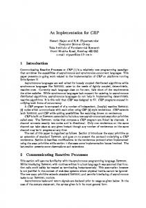
day time frames and in 785 out of 929 bands. The distribution of good data segments in time frames and in bands is given in Figure 3. In Figure 4 we plot a snapshot spectral density of VSR1 data presented in Figure 1 and an estimate of the spectral density of the data that was used in the analysis. We estimate the spectral density in each band by a harmonic mean of the spectral densities of each of the two-day time segments chosen for the analysis in the band. As the data spectrum in each band is approximately white, we estimate the spectral density in each time segment by 2σ 2 ∆t, where σ 2 is the variance of the data in a segment and ∆t is the 1/2s sampling time. We plot the band from 100Hz to 1 kHz which we have chosen for this search. 4. The response of the detector The dimensionless noise-free response h of a gravitational-wave detector to a weak plane gravitational wave in the long wavelength approximation, i.e., when the characteristic size of the detector is much smaller than the reduced wavelength λ/(2π)

50

550

45

500

40

450

35

400

Bands Number

Time Frames Number

F -statistic all-sky search for continuous gravitational waves in Virgo data

30 25 20 15

13

350 300 250 200 150

10

100

5

50

0 0

100

200

300

400

500

600

700

800

0

Sorted band index

0

5

10

15

20

25

30

35

40

45

50

Sorted frame index

Figure 3. Number of good data segments. Left panel - distribution of data segments in frequency bands. The number of data segments chosen for the analysis in a given frequency band varies from 1 to 50. Right panel - distribution of data segments time frames. The number of data segments in a given time frame varies from 54 to 520. The smallest, outlying number of bands of 54 is in the 5th time frame. In the remaining frames the number of good bands is greater than 300. −19

10

25th May 2007 VSR1 good data

−20

S

1/2 −1/2 [Hz ] h

10

−21

10

−22

10

100

200

300

400

500 600 Frequency [Hz]

700

800

900

1000

√ Figure 4. A snapshot of strain amplitude spectral density Sh of the VSR1 data (grey curve) in comparison with the spectral density estimated from the data used in the analysis (black dots). The spectrum in each band is obtained from a harmonic mean of the spectral densities of the data in each segment chosen for the analysis in the band.

of the wave, can be written as the linear combination of the two independent wave polarizations h+ and h× , h(t) = F+ (t)h+ (t) + F× (t)h× (t),

(2)

where F+ and F× are the detector’s beam-pattern functions, F+ (t) = a(t) cos 2ψ + b(t) sin 2ψ,

(3)

F -statistic all-sky search for continuous gravitational waves in Virgo data F× (t) = b(t) cos 2ψ − a(t) sin 2ψ.

14 (4)

The beam-patterns F+ and F× are linear combinations of sin 2ψ and cos 2ψ, where ψ is the polarization angle of the wave. The functions a(t) and b(t) are the amplitude modulation functions, that depend on the location and orientation of the detector on the Earth and on the position of the gravitational-wave source in the sky, described in the equatorial coordinate system by the right ascension α and the declination δ angles. They are periodic functions of time with the period of one and two sidereal days. The analytic form of the functions a(t) and b(t) for the case of interferometric detectors is given by Eqs. (12) and (13) of [18]. For a rotating nonaxisymmetric neutron star, the wave polarization functions are of the form h+ (t) = h0+ cos(φ(t) + φ0 ),

h× (t) = h0× sin(φ(t) + φ0 ),

(5)

where h0+ and h0× are constant amplitudes of the two polarizations and φ(t) + φ0 is the phase of the wave, φ0 being the initial phase of the waveform. The amplitudes h0+ and h0× depend on the physical mechanism responsible for the gravitational radiation, e.g., if a neutron star is a triaxial ellipsoid rotating around a principal axis with frequency f , then these amplitudes are 1 h0× = h0 cos ι, (6) h0+ = h0 (1 + cos2 ι), 2 where ι is the angle between the star’s angular momentum vector and the direction from the star to the Earth, and the amplitude h0 is given by 16π 2 G ǫIf 2 . (7) c4 r Here I is the star’s moment of inertia with respect to the rotation axis, r is the distance to the star, and ǫ is the star’s ellipticity defined by ǫ = |I1 − I2 |/I, where I1 and I2 are moments of inertia with respect to the principal axes orthogonal to the rotation axis. We assume that the gravitational waveform given by Eqs. (2)– (5) is almost monochromatic around some angular frequency ω0 , which we define as instantaneous angular frequency evaluated at the solar system barycenter (SSB) at t = 0, and we assume that the frequency evolution is accurately described by one spindown parameter ω1 . Then the phase φ(t) is given by h0 =

n · rd (t) (ω0 + 2ω1 t), (8) c where, neglecting the relativistic effects, rd (t) is the vector that joins the SSB with the detector, and n is the unit vector pointing from SSB to the source. In equatorial coordinates (δ, α) we have n = (cos δ cos α, cos δ sin α, sin δ). φ(t) = ω0 t + ω1 t2 +

5. The F - statistic A method to search for gravitational wave signals from a rotating neutron star in a detector data x(t), t = 1, ..., N uses the F -statistic, described in [18]. The F -statistic is obtained by maximizing the likelihood function with respect to the four unknown parameters - h0 , φ0 , ι, and ψ. This leaves a function of only the remaining four parameters - ω0 , ω1 , δ, and α. Thus the dimension of the parameter space that we need to search decreases from 8 to 4. In this analysis we shall use an observation time Tobs equal to the integer multiple of sidereal days. Since the bandwidth of the signal over our coherent observation time of two days is very small, we can assume

F -statistic all-sky search for continuous gravitational waves in Virgo data

15

that over this band the spectral density of the noise is white (constant). Under these assumptions the F -statistic is given by [26, 27]   2 |Fa |2 |Fb |2 F≈ 2 , (9) + 2 σ ha2 i hb i where σ 2 is the variance of the data, and Fa :=

N X

x(t) a(t) exp[−iφ(t)],

N X

x(t) b(t) exp[−iφ(t)].

(10)

t=1

Fb :=

t=1

N N

2 X

 X a = a(t)2 , b2 = b(t)2 . t=1

(11)

t=1

6. Description of the search The search consists of two parts; the first part is a coherent search of two-day data segments, where we search a 4-parameter space defined by angular frequency ω0 , angular frequency derivative ω1 , declination δ, and right ascension α. The search is performed on a 4-dimensional grid in the parameter space described in Section 6.2. We set a fixed threshold of 20 for the F -statistic for each data segment. This corresponds to a threshold of 6 for the signal-to-noise ratio. All the threshold crossings are recorded together with corresponding 4 parameters of the grid point and the signal-to-noise ratio ρ. The signal-to-noise is calculated from the value of the F -statistic at the threshold crossing as p (12) ρ = 2(F − 2). In this way for each narrow band segment we obtain a set of candidates. The candidates are then subject to the vetoing procedure described in Section 7. The second part of the search is the post-processing stage involving search for coincidences among the candidates. The coincidence procedure is described in Section 8. 6.1. Choice of the parameter space We have searched the frequency band from 100 Hz to 1 kHz over the entire sky. We have followed [13] to constrain the maximum value of the parameter ω1 for a given frequency ω0 by |ω1 | ≤ ω0 /(2τmin ), where τmin is the minimum spindown age‡. We have chosen τmin = 1000yr for the whole frequency band searched. Also, in this search we have considered only the negative values for the parameter ω1 , thus assuming that the rotating neutron star is spinning down. This gives the frequency-dependent range of the spindown parameter f1 where f1 = ω1 /(2π): f 1000yr [Hzs−1 ] (13) 100Hz τmin We have considered only one frequency derivative. Estimates taking into account parameter correlations (see [13] Figure 6 and Eqs. (6.2) - (6.6)) show that even for |f1 | ≤ 1.6 × 10−9

‡ The factor of two in this formula appears here because the spindown parameter f˙ used in [13] is twice the spindown parameter used in this work.

F -statistic all-sky search for continuous gravitational waves in Virgo data

16

Frequency derivative [10−8 Hz/s]

0.0 −0.5 −1.0 −1.5 −2.0 −2.5 −3.0 0

PowerFlux (early S5) PowerFlux (full S5) F-stat (VSR1) E@H (early S5) E@H (full S5)

200

400

600

800

1000

Frequency [Hz]

1200

1400

1600

Figure 5. Comparison of the parameter space in f − f˙ plane searched in VSR1 analysis presented in this paper (area enclosed by a thick black line) and recently published PowerFlux and E@H searches of the LIGO S5 data.

the minimum spindown age of 40yr and for two days coherent observation time that we consider here, it is sufficient to include just one spindown parameter. In Figure 5 we have compared the parameter space searched in this analysis in the f − f˙ plane with that of other recently published all-sky searches: Einstein@Home early S5 search [21], Einstein@Home full S5 [22], PowerFlux early S5 [28], PowerFlux full S5 [17]. 6.2. Efficient calculation of the F -statistic on the grid in the parameter space Calculation of the F -statistic (Eq. (9)) involves two sums given by Eqs. (10). By introducing a new time variable called the barycentric time tb ([29, 18, 27]) n · rd (t) . c we can write these sums as discrete Fourier transforms in the following way tb := t +

Fa =

N X

x(t(tb )) a(t(tb )) exp[−iφs (t(tb ))] exp[−iω0 tb ],

N X

x(t(tb )) b(t(tb )) exp[−iφs (t(tb ))] exp[−iω0 tb ],

(14)

(15)

tb =1

Fb =

tb =1

where n · rd (t) ω1 t. (16) c Written in this form, the two sums can be evaluated using the Fast Fourier Transform (FFT) algorithm thus speeding up their computation dramatically. The time φs (t) = ω1 t2 + 2

F -statistic all-sky search for continuous gravitational waves in Virgo data

17

transformation described by equation (14) is called resampling. In addition to the use of the FFT algorithm we apply an interpolation of the FFT using the interbinning procedure (see [27] Section VB). This results in the F -statistic sampled twice as fine with respect to the standard FFT. This procedure is much faster than the interpolation of the FFT obtained by padding the data with zeroes and calculating a FFT that is twice as long. With the approximations described above for each value of the parameters ω1 , δ, and α, we calculate the F -statistic efficiently for all the frequency bins in the data segment of bandwidth 1Hz. In order to search the 4-dimensional parameter space, we need to construct a 4-dimensional grid. To minimize the computational cost we construct a grid that has the smallest number of points for a certain assumed minimal match M M [30]. This problem is equivalent to the covering problem [31, 32] and it has the optimal solution in 4-dimensions in the case of a lattice i.e., a uniformly spaced grid. In order that our parameter space is a lattice, the signals’ reduced Fisher matrix must have components that are independent of the values of the parameters. This is not the case for the signal given by Eqs. (2) - (8); it can be realized however for an approximate signal called the linear model described in Section IIIB of [27]. The linear model consists of neglecting amplitude modulation of the signal and discarding the component of the vector rd (t) joining the detector and the solar system barycenter that is perpendicular to the ecliptic. This approximation is justified because the amplitude modulation is very slow compared to the phase modulation and the discarded component in the phase is small compared to the others. As a result the linear model signal hlin (t) has a constant amplitude A0 , and one can find parameters such that the phases are linear functions of them. We explicitly have (see Section IIIB of [27] for details): hlin (t) = A0 cos[φlin (t) + φ0 ],

(17)

φlin (t) = ω0 t + ω1 t2 + α1 µ1 (t) + α2 µ2 (t).

(18)

where The parameters α1 and α2 are defined by α1 := ω0 (sin α cos δ cos ε + sin δ sin ε),

(19)

α2 := ω0 cos α cos δ,

(20)

where ε is the obliquity of the ecliptic, and µ1 (t) and µ2 (t) are known functions of the detector ephemeris. In order that the grid is compatible with application of the FFT, its points should be constrained to coincide with Fourier frequencies at which the FFT is calculated. Moreover, we observed that a numerically accurate implementation of the interpolation to the barycentric time (see Eq. (14)) is so computationally demanding that it may offset the advantage of the FFT. Therefore we introduced another constraint in the grid such that the resampling is needed only once per sky position for all the spindown values. Construction of the constrained grid is described in detail in Section IV of √ [27]. In this search we have chosen the value of the minimal match M M = 3/2. The workflow of the coherent part of the search procedure is presented in Figure 6. 7. Vetoing procedure We apply three vetoing criteria to the candidates obtained in the coherent part of the search - line width veto, stationary line veto and polar caps veto. Data from the

F -statistic all-sky search for continuous gravitational waves in Virgo data

18

Figure 6. Workflow of the F -statistic search pipeline.

detector always contain some periodic interferences (lines) that are detector artifacts. An important part of our vetoing procedure was to identify the lines in the data. We have therefore performed a Fourier search with frequency resolution of 1/(2 days) ≃ 5.8 × 10−6 Hz for periodic signals of each of the two-day data segments. We compared the frequencies of the significant periodic signals identified by our analysis with the line frequencies obtained by the Virgo LineMonitor and we found that all the lines from the LineMonitor were detected by our Fourier search. 7.1. Line width veto We veto all the candidates with frequency f around every known line frequency fl according to the following criterion |f − fl | < ∆fmax ,

(21)

where the width ∆fmax is estimated as ∆fmax = fl |v|max /c + 2|f1 |max (Tobs + Tobs |v|max /c + |r|max /c), (22)

where vmax is the maximum value of the velocity of the detector with respect to the SSB during the observation time, rmax is the maximum distance to the SSB during the

F -statistic all-sky search for continuous gravitational waves in Virgo data

19

coherent observation time Tobs , and |f1 |max is the maximum of the absolute value of the frequency derivative. Eq. (22) determines the maximum smearing of the frequency on each side of the line due to frequency modulation induced by the filters applied in the F -statistic. 7.2. Stationary line veto Let us consider the instantaneous frequency finst of the signal, i.e., the time derivative of the phase: 1 dφ(t) n · vd (t) n · rd (t) = f0 + 2f1 t + (f0 + 2f1 t) + 2 f1 , (23) 2π dt c c where vd (t) = drd (t)/dt. The frequency derivative of the instantaneous frequency is given by finst :=

n · ad (t) n · vd (t) dfinst (t) = 2f1 + (f0 + 2f1 t) + 4 f1 , (24) dt c c where ad (t) = dvd (t)/dt. Eq. (24) is the rate of change of detector response frequency for a source whose SSB frequency and spindown are f0 and f1 . An instrumental line has a constant detector frequency and mimics a source for which the r.h.s of Eq. (24) vanishes. In practice, we veto candidates with 2 2 2f1 + n · ad (t) f0 + 2 n · d (rd (t)t)/dt f1 < ǫSL (25) c c

for some ǫSL > 0. In the search we choose ǫSL = 1/Tobs 2 , where Tobs is the observation time. The above stationary line veto was introduced in reference [14] and refined in [33]; it was used in the first two E@H searches [20, 21]. 7.3. Polar caps veto

We observe that many of the detected lines cluster around the poles where declination δ is close to ±π/2. An interference originating from a detector will correlate well with our templates if the frequency modulation in Eq. (23) is minimized. Assuming that f1 = 0 and that the diurnal motion of the Earth averages to 0 over two days observation time, this happens when the quantity |n·vd (t)| is minimized. We find that this quantity is close to minimum independently of the value of α when δ = ±π/2. Thus we veto candidates that are too close to the poles; we discard all candidates with the declination angle δ within three grid cells from the poles. 8. Coincidences In order to find coincidences among the candidates, we applied a method similar to the one used in the first two E@H searches [20, 21]. For each band we have searched for coincidences among candidates in different time frames. We are able to search for coincidences only in those bands where there were two or more time frames with data selected for the analysis. If we search for a real gravitational wave signal, we must take into account frequency evolution due to spindown of the rotating neutron star. Thus the first step in the coincidence analysis was to transform all frequencies ω0 (tl ) of the candidates to a common fiducial reference time tf . We have chosen the fiducial

F -statistic all-sky search for continuous gravitational waves in Virgo data

20

time to be the time of the first sample of the latest time frame that we analyzed i.e., the 67th time frame. We have ω(tf ) = ω0 (tl ) + 2 ω1 (tl )[67 Tobs − tl ],

(26)

where tl is the time of the first sample of the lth time frame. The next step was to divide the parameter space into cells. This construction of the coincidence cell was different from that in the E@H analysis. To construct the cells in the parameter ˜ for the linear signal model defined by space we have used the reduced Fisher matrix Γ Eqs. (17) and (18). The reduced Fisher matrix is the projected Fisher matrix on the 4-dimensional space spanned by parameters κ = (ω0 , ω1 , α1 , α2 ). We define the cell in the parameter space by the condition: X ˜ kl κk κl ≤ 2. Γ (27) k,l

Because the ephemeris of the detector is different in each of the time frames, the reduced Fisher matrix is different in each time frame. To have a common coincidence grid we have chosen the grid defined by the latest frame i.e., the frame no. 67 as the coincidence grid. After the transformation of the candidate frequencies to a reference time and construction of the coincidence grid, the coincidence algorithm for each of the bands proceeded in the following steps: 1. Transform angles α and δ to α1 and α2 coordinates (see Eq.(19)) 2. Transform candidate parameters to xl coordinates defined by xl =

4 X

√ κk Vkl el ,

(28)

k=1

˜ and el are its eigenvalues. where Vkl , k = 1, .., 4 are eigenvectors of the matrix Γ, In these coordinates the Fisher matrix is proportional to the unit matrix. 3. Coordinates xl are rounded to the nearest integer. In this way we sort candidates efficiently into adjacent 4-dimensional hypercubes. If there are more than one candidates from a given data segment in a hypercube we select the candidate that has the highest SNR. We do sorting for each time frame in the band. If there is more than one candidate in a given hypercube we register a coincidence. 4. We shift cubes by 1/2 of their size in all possible 24 directions, and for each shift we search for coincidences. This last step of the algorithm takes into account cases for which the candidate events are located on opposite sides of cell borders, edges, and corners and consequently coincidences that could not be found just by packing candidates into adjacent cells. The most significant coincidence in each band is the one which has the highest multiplicity. For each most significant coincidence we have calculated the false alarm probability i.e., the probability that such a coincidence can occur purely by chance. The false alarm probability is calculated using the formula explained in Appendix A and given by Eq. (A.6). This general formula applies to a variable number of candidates in various time slots and also takes into account the 24 shifts of the cells in the parameter space.

F -statistic all-sky search for continuous gravitational waves in Virgo data

21

9. The search In this analysis we have searched coherently 20 419 two-day time segments of data narrowbanded to 1 Hz. In the coherent part of the search described in Section 6 we have used 9.10 × 1016 templates which is the number of F -statistic values computed. This resulted in 20 419 candidate files containing 4.21 × 1010 candidates. The candidates were subject to the vetoing using the three veto criteria: line veto, polar caps veto, and stationary line veto described in Section 7. As a result of vetoing around 24% of the candidates were discarded leaving 3.19 × 1010 candidates. Nearly all candidates were vetoed by the line veto, whereas 0.20% were vetoed by the stationary line criterion and only 3.2 × 10−2 % by the polar caps veto. In Figure 7 we present an example of the candidate distribution obtained from the coherent search of one narrow band data segment and after the vetoing procedure. In the

Candidates in data segment: 30−089 Histogram of candidates

0.05

0.15

0 −0.05

0.1 0

5

10 Time [s]

15 4

x 10

−22.2

0.05

−22.4 −22.6 186.4

186.6 186.8 Frequency [Hz]

187

0

187.2

45

Frequency distribution

50 55 2 × F−statistic

60

Distribution on the sky

8.5 8 7.5 7

7

0

6.5

−50

6.5 6

7.5

50 δ [deg]

Signal−to−noise

Spectral density [Hz−1/2] Amplitude

Time series

186.4

186.6 186.8 Frequency [Hz]

187

187.2

0

100

200 α [deg]

300

Figure 7. Distribution of candidates after vetoing obtained in the coherent F statistic search of two-day data segment 30 − 089 i.e., a segment with the time frame number d = 30 and the band number b = 89. The left top panel shows data and its spectrum. The right top panel shows the distribution of 2F values of the candidates in comparison to the χ2 distribution with 4 degrees of freedom. The bottom left panel shows the distribution of signal-to-noise ratios ρ (see Eq. (12)) of the candidates as a function of the frequency. The vertical black line is the periodic interference identified in the data. The candidates in the band around the line are vetoed (see Eq. (22)). The right bottom panel shows the distribution of the candidates on the sky in equatorial coordinates α and δ. The distribution shows singularity at the ecliptic. This is a consequence of the grid construction from the approximate linear signal model given by Eqs.(17) - (19).

F -statistic all-sky search for continuous gravitational waves in Virgo data

22

next step we have searched for the significant coincidences among the candidates. We have searched for coincidences in all the frequency bands where there were two or more data segments analyzed. In Figure 8 we have plotted the highest coincidence multiplicity for each of the bands. The highest multiplicity was 6, and it occurred in 10 bands. The multiplicity tends to grow with the frequency, because the size of the parameter space grows as f 3 . For each band we have calculated the false alarm VSR1 all sky search

Coincidence multiplicity

6

5

4

3

2 100

200

300

400

500

600

700

800

900

1000

200

300

400

500 600 Frequency [Hz]

700

800

900

1000

False alarm probablity

1 0.8 0.6 0.4 0.2 0 100

Figure 8. Coincidences among the candidates. Top panel: maximum multiplicity of coincidence as function of frequency. Bottom panel: corresponding coincidence false alarm probability.

probability corresponding to the most significant coincidence using Eq. (A.6). The most significant coincidence occurred in band no. 401, corresponding to the frequency range of ∼ [488.4, 489.4] Hz. It was a coincidence of multiplicity = 5, and its false alarm probability was 14.5%. Note that a coincidence with the highest multiplicity is not the most significant. This is because the significance depends on the number of time frames with candidates in a given band and also on the number of candidates in the time frames. By adopting a criterion used by E@H searches that the background coincidences correspond to false alarm probability of 0.1% or greater, we conclude that we have found no significant coincidence and thus no viable gravitational wave candidate. Considering the significance of the coincidences, we could adopt even a 10% false alarm probability as a background. Consequently, we proceed to the final stage of our analysis - estimation of sensitivity of the search. 10. Sensitivity of the search The sensitivity of the search is taken to be the amplitude h0 of the gravitational wave signal that can be confidently detected. To estimate the sensitivity we use a procedure developed in [20]. We determine the sensitivity of the search in each of

F -statistic all-sky search for continuous gravitational waves in Virgo data

23

the 785 frequency bands that we have searched. To determine the sensitivity, we perform Monte Carlo simulations in which, for a given amplitude h0 , we randomly select the other seven parameters of the signal: ω0 , ω1 , α, δ, φ0 , ι, and ψ. We choose frequency and spindown parameters uniformly over their range, and source positions uniformly over the sky. We choose angles φ0 and ψ uniformly over the interval [0, 2π] and we choose cos ι uniformly over the interval [−1, 1]. For each band we add the signal to all the data segments chosen for the analysis in that band. Then we process the data through our pipeline. First, we perform a coherent F -statistic search of each of the data segments where the signal was added, and store all the candidates above our F -statistic threshold of 20. In this coherent analysis, to make the computation manageable, we search over only parameter space consisting of ± 2 grid points around the nearest grid point where the signal was added. Then we apply our vetoing procedure to the candidates obtained as explained in Section 7. Finally, we perform coincidence analysis of the candidates that survive vetoing which is described in Section 8. We define a detectable signal if it is coincident in more than 70% of the time frames in a given band. This condition is similar to the condition used in the two E@H searches, where a coincidence method was used [20, 21]. For bands with only one frame available the coherent search over one 2-day data segment was performed. In this case the injected signal is declared detected if its signal-to-noise ratio obtained in the coherent search is larger than the signal-to-noise ratio of the loudest signal in that data segment without an injection. For each band we inject signals with 5 different amplitude values, and perform 100 randomized injections for each amplitude. For each amplitude we calculate how many signals were detected, and by interpolation we determine the amplitude corresponding to 90% of signals detected. This amplitude was defined as the 90% confidence sensitivity. Sometimes even for the highest amplitude we have not reached the 90% detection probability. In this case we performed injections for higher amplitudes until the desired level of detectability was achieved. In Figure 9, as an example, we present an estimation of the sensitivity in the band b = 369 corresponding to the frequency range of ∼ [457.47, 458.44] Hz. The errors in the sensitivity estimates originate from calibration errors in the amplitude and errors due to a finite number of Monte Carlo injections. We use 100 injections; hence from a binomial statistic, one σ is equivalent to 3% fluctuation. Thus the estimated amplitude sensitivity corresponds to confidence in the range from 87% to 93%. To estimate how this uncertainty in confidence translates into uncertainty in the amplitude we have performed an additional set of injections for a range of amplitudes close to the estimated sensitivity and from the slope of the confidence vs. amplitude we determined the uncertainty in the amplitude. To increase the accuracy of the error estimate, we have performed 1000 injections for each amplitude. The uncertainty in the amplitude was not more than 5%. The calibration errors in VSR1 data are 6% (see Section 2). Adding these two types of errors in quadrature results in the total error in sensitivity estimate to be around 7%. The sensitivity of this search obtained through Monte Carlo simulations for the whole band searched is presented in Figure 10. We see from Figure 10 that the sensitivity essentially reflects the instrumental noise curve given in Figure 4. We have made a fit of the sensitivity h90% to the one-sided spectral 0 density Sh (f ) of detector noise described by the following relation: r Sh (f ) 90% . (29) h0 = RD 48 hours

F -statistic all-sky search for continuous gravitational waves in Virgo data

24

Sensitivity for the band no. 369. No. of frames = 20 1

0.9

0.8

Detection probability

0.7

0.6

0.5

0.4

0.3

0.2

0.1 90% confidence sensiivity 0

0

1

2

3

4 5 Source strain smplitude h

o

6

7

8 −24

x 10

Figure 9. Estimation of sensitivity in the band no. 369. In this band there are 20 time frames. Thus the signal is detected if it is coincident in more than 14 frames. The black dots are amplitudes of the injected signals and the corresponding detection probabilities estimated from the injections. The red circle is the interpolated amplitude corresponding to 90% detection probability. This is the 90% confidence sensitivity for this band.

We find that the prefactor RD is in the range from 15.6 to 22.4 and it depends on the frequency band and the number of the data segments in the band. 11. Conclusions The sensitivity of this search was 50% to 2 times better, depending on the bandwidth, than that of the LIGO S4 search [20] and comparable to the sensitivities obtained in the early LIGO S5 data [21], but 2 to 5 times worse than the upper limits in the E@H full LIGO S5 data search [22]. This was due to the lower noise and longer observation time for the LIGO S5 data w.r.t the Virgo VSR1 data. However, for the first time in an all-sky search we have estimated the sensitivity in the frequency band from 400Hz to 1kHz and the frequency spindown range from −7.2 (f0 /400 Hz) × 10−9 Hz/s to −6.0 × 10−9 Hz/s, which is a previously unexplored region in the parameter space. The next step is to test the search method described in this paper in the Mock Data Challenge (MDC) designed by the LIGO and Virgo projects to validate and compare pipelines that are proposed to be used in the analysis of the forthcoming data from the advanced detectors. It is also planned to further test the pipeline presented here with other data sets collected by the LIGO and Virgo detectors.

F -statistic all-sky search for continuous gravitational waves in Virgo data −23

4.5

25

VSR1 all−sky search: sensitivity

x 10

Sensitivity Rescaled noise curve 4

3.5

Sensitivity

3

2.5

2

1.5

1

0.5

0 100

200

300

400

500 600 Frequency [Hz]

700

800

900

1000

Figure 10. The 90% confidence sensitivity of the all-sky search of Virgo VSR1 data in the band from 100 Hz to 1 kHz. The dots show the source strain amplitude h0 for which 90% of sources are confidently detected by this pipeline. The thin line is the rescaled instrumental noise curve, see Eq. (29).

Acknowledgments The authors gratefully acknowledge the support of the United States National Science Foundation for the construction and operation of the LIGO Laboratory, the Science and Technology Facilities Council of the United Kingdom, the Max-Planck-Society, and the State of Niedersachsen/Germany for support of the construction and operation of the GEO600 detector, and the Italian Istituto Nazionale di Fisica Nucleare and the French Centre National de la Recherche Scientifique for the construction and operation of the Virgo detector. The authors also gratefully acknowledge the support of the research by these agencies and by the Australian Research Council, the International Science Linkages program of the Commonwealth of Australia, the Council of Scientific and Industrial Research of India, the Istituto Nazionale di Fisica Nucleare of Italy, the Spanish Ministerio de Econom´ıa y Competitividad, the Conselleria d’Economia Hisenda i Innovaci´ o of the Govern de les Illes Balears, the Foundation for Fundamental Research on Matter supported by the Netherlands Organisation for Scientific Research, the Polish Ministry of Science and Higher Education, the FOCUS Programme of Foundation for Polish Science, the PL-Grid Infrastructure, the Royal Society, the Scottish Funding Council, the Scottish Universities Physics Alliance, The National Aeronautics and Space Administration, the Carnegie Trust, the Leverhulme Trust, the David and Lucile Packard Foundation, the Research Corporation, and the Alfred P. Sloan Foundation. This document has been assigned LIGO Laboratory document number LIGO-P1300133.

F -statistic all-sky search for continuous gravitational waves in Virgo data

26

References [1] [2] [3] [4] [5] [6] [7] [8] [9] [10] [11] [12] [13] [14] [15] [16] [17] [18] [19] [20] [21] [22] [23] [24] [25] [26] [27] [28] [29] [30] [31] [32] [33]

T Accadia et al 2012 JINST 7 P03012 B Abbott et al 2007 Phys. Rev. D76 082001 A Mastrano, P D Lasky and A Melatos 2013 (Preprint 1306.4503) B J Owen 2010 Phys. Rev. D 82 104002 D J Jones and N Andersson 2001 Mon. Not. R. Astron. Soc. 331 203 L Bildsten 1998 Astrophys. J. 501 L89 G Ushomirsky, C Cutler and L Bildsten 2000 Mon. Not. R. Astron. Soc. 319 902 C Cutler 2002 Phys. Rev. D 66 084025 A Melatos and D J B Payne 2005 Astrophys. J. 623 1044 B J Owen 2005 Phys. Rev. Lett. 95 211101 N K Johnson-McDaniel and B J Owen 2013 Phys. Rev. D 88 044004 C J Horowitz and K Kadau 2009 Phys. Rev. Lett. 102 191102 P R Brady, T Creighton, C Cutler and B F Schutz 1998 Phys. Rev. D 57 2101 B Abbott et al 2008 Phys. Rev. D77 022001 B Abbott et al 2005 Phys. Rev. D 72 102004 B Abbott et al 2009 Phys. Rev. Lett. 102 111102 J Abadie et al 2012 Phys. Rev. D85 022001 P Jaranowski, A Kr´ olak and B Schutz 1998 Phys. Rev. D 58 063001 http://einstein.phys.uwm.edu B Abbott et al 2009 Phys. Rev. D79 022001 B Abbott et al 2009 Phys. Rev. D80 042003 J Aasi et al 2013 Phys. Rev. D87 042001 F Acernese et al 2008 Class. Quant. Grav. 25 184001 T Accadia et al 2010 Journal of Physics: Conference Series 228 012015 P Astone et al 2002 Phys. Rev. D 65 022001 P Astone, K M Borkowski, P Jaranowski and A Kr´ olak 2002 Phys. Rev. D 65 042003 P Astone, K M Borkowski, P Jaranowski, M Pietka and A Kr´ olak 2010 Phys. Rev. D 82 022005 B Abbott et al 2009 Phys. Rev. Lett. 102 111102 B F Schutz The Detection of Gravitational Waves ed Blair D (Cambridge University Press) B Owen 1996 Phys. Rev. D 53 6749 J H Conway and N J A Slone 1999 Sphere packings, lattices and groups (New York: Springer) Prix R 2007 Phys. Rev. D 75 023004 H J Pletsch 2008 Phys. Rev. D 78 102005

Appendix A. False alarm coincidence probability Let us assume that for a given frequency band we analyze L non-overlapping time segments. Suppose that the search of the lth segment produces Nl candidates. Let us assume that the size of the parameter space for each time segment is the same, and it can be divided into the number Ncell of independent cells. We would like to test the null hypothesis that coincidences among candidates from L segments are accidental. The probability for a candidate event to fall into any given coincidence cell is equal to 1/Ncell. Thus probability ǫl that a given coincidence cell is populated with one or more candidate events is given by  1 Nl . (A.1) ǫl = 1 − 1 − Ncell We may also consider independent candidates only, i.e., such that there is no more than one candidate within one cell. If we obtain more than one candidate within a given cell we choose the one which has the highest signal-to-noise ratio. In this case Nl ǫl = . (A.2) Ncell The probability pF (Ncell ) that any given coincidence cell out of the total of Ncell cells contains candidate events from Cmax or more distinct data segments is given by a

F -statistic all-sky search for continuous gravitational waves in Virgo data

27

generalized binomial distribution pF (Ncell ) =

L X

n=Cmax

×

X

σ∈Π(L)

1 × n!(L − n)!

ǫσ(1) . . . ǫσ(n) (1 − ǫσ(n+1) ) . . . (1 − ǫσ(L) ),

(A.3)

P where σ∈Π(L) is the sum over all the permutations of the L data sequences. Finally the probability PF that there is Cmax or more coincidences in one or more of the Ncell cells is PF = 1 − (1 − pF (Ncell ))Ncell .

(A.4)

PF = 1 − (1 − (2pF (Ncell ) − pF (2Ncell)))Ncell .

(A.5)

The above formula for the false alarm coincidence probability does not take into account the case when candidate events are located on opposite sides of cell borders, edges, and corners. In order to find these coincidences the entire cell coincidence grid is shifted by half a cell width in all possible 24 = 16 combinations of the four parameter-space dimensions, and coincidences are searched in all the 16 coincidence grids. This leads to a higher number of accidental coincidences, and consequently Eq. A.4 underestimates the false alarm probability. Let us consider the simplest onedimensional case. In this case we have 21 = 2 possible shifts (the original coincidence grid and the one shifted by half). This increases probability pF (Ncell ) by a factor of 2 if the two cell coincidence grids were independent. However the cells overlap by half and some coincidences would be counted twice. To account for this we divide the cells in the coincidence grid by half resulting in 2Ncell cells and define the false alarm probability pF (2Ncell) that any given half of the coincidence cell out of the total of 2Ncell half cells contains candidate events from Cmax or more distinct data segments. These are coincidences that were already counted, and consequently the false alarm probability with the cell shift is 2pF (Ncell )− pF (2Ncell). This results in the false alarm probability To generalize the above formula to higher dimensions we need to consider further shifts and divisions of the cells. In the four dimension case this leads to the formula for the probability PFshifts that there are Cmax or more independent coincidences in one or more of the Ncell cells in all 16 grid shifts given by h  PFshifts = 1 − 1 − 24 pF (Nc ) (A.6)        
4 4 4 4 pF (2Nc ) + pF (22 Nc ) + − pF (23 Nc ) + pF (24 Nc ) 1 2 3 4      
4 4 4 pF (22 Nc ) + pF (23 Nc ) + pF (24 Nc ) − 2 3 4    
4 4 pF (23 Nc ) + pF (24 Nc ) − 3 4   i N c 4 pF (24 Nc ) − 4 By choosing a certain false alarm probability PF , we can calculate the threshold number Cmax of coincidences. If we obtain more than Cmax coincidences in our search we reject the null hypothesis that coincidences are accidental only at the significance level of PF .