compliance. The displacement used in the load vs. displacement curve can be
defined either as the load- ... specimen according to the standard BS 7448-1 [13].
Sustainable Construction and Design 2011
IMPLEMENTATION OF AN UNLOADING COMPLIANCE PROCEDURE FOR MEASUREMENT OF CRACK GROWTH IN PIPELINE STEEL K. Van Minnebruggen1, D. Van Puyvelde1, W. De Waele1, M. Verstraete1, S. Hertelé1,2, R. Denys1 1 2
Ghent University, Laboratory Soete, Belgium FWO (Flanders Research Foundation) aspirant
Abstract As the demand for fossil fuels increases, pipelines are constructed in inhospitable areas. Under these conditions, not only the strength but also the deformability of the pipelines becomes crucial. A strain based design (SBD) procedure needs to be established. Traditional stress based approaches to evaluate defect tolerance lead to conservative predictions. There is a need to accurately define the fracture toughness of the pipeline steel and assess the criticality of weld defects under strain based conditions. This paper focuses on the implementation of the unloading compliance method to determine stable crack growth. The standardized test procedure described in ASTM E1820 is applied. This method is a handy tool to obtain the J-resistance curves which can forecast ductile failure in pipeline girth welds. Preliminary experiments have been performed on Single Edge Notch Bend (SENB) specimens of plain pipe metal. Using the implemented procedure, it was possible to obtain a good fit between calculated and measured crack size. The most important result is the smoothness of the calculated crack growth and the rather monotonic increase of crack size. Since testing on SENB is well known to provide conservative measurements, Single Edge Notch Tension (SENT) specimens will be evaluated in future work. Keywords Strain based design, Unloading Compliance method, crack growth, resistance curve 1
INTRODUCTION
Conventional pipeline design is based on a so-called stress design approach, which limits the applied stress to a prescribed fraction of the material’s minimum specified yield strength. Recently built pipelines often have to traverse challenging environments, featuring hazards such as permafrost, seismic, land slide prone terrains, or require operations with extreme thermal/pressure fluctuations [1]. These situations could cause a longitudinal plastic deformation beyond the pipe’s yield strain allowed by the limits in the commonly used design codes and standards [2, 3]. Therefore, a strain based design approach, which allows a certain amount of plastic strain, is more suitable. This is particularly true for applications where the loading is displacement controlled and the maximum resulting strain is bounded. For example, such displacement controlled plastic straining of pipes occurs in pipe reeling and laying [4]. Welding pipes together unavoidably involves the presence of weld defects. It is not possible to detect or accurately size all defects with non-destructive inspection, and due to economical reasons these cannot all be repaired. Moreover, some defects can possibly be tolerated based on fracture mechanics assumptions. To determine a maximum allowable defect size, accurate knowledge of material properties, and specifically fracture toughness is needed. In strain based conditions, the defective weld will be subjected to high plastic strains and ductile tearing will inevitably occur. For such problems the fracture resistance curve, i.e. the relation of toughness versus ductile crack growth, has to be determined. A material’s fracture resistance curve displays the energy needed (J-integral) for a certain crack extension ('a). This curve can be combined with the crack driving force (CDF) curve. The CDF expresses the applied energy for varying crack lengths at a given load level (displacement or force). This CDF curve can be determined by either finite element analysis (FEA) or analytical solutions [5, 6]. A comparison of both curves results in the maximum applicable load before unstable failure occurs. In Figure 1 this maximum load corresponds to the load level P 3 . This paper focuses on the experimental determination of ductile crack growth and resistance curves. Preliminary Single Edge Notch Bend (SENB) tests have been performed on plain pipe material. Although these tests are widely known to give over conservative predictions when applied to pipeline design [7, 8], the economical benefits in terms of test rig capacity and needed material make the SENB test very suitable for the evaluation of the implemented method for characterization of ductile crack growth.
397
Copyright © 2011 by Laboratory Soete
Sustainable Construction and Design 2011
Figure 1: Fracture resistance curve (dashed line) and crack driving force curves (full lines) to determine the maximum allowable load. 2
THE UNLOADING COMPLIANCE PROCEDURE
Several methods are available to determine ductile crack growth, for example the potential drop method [9] or the silicone replica technique [10]. Another frequently used technique is the unloading compliance (UC) method. This standardized method is explained in detail in the following subparagraphs. 2.1
Background
The compliance, C, can be defined as the inverse slope of the elastic unloading part on the load vs. displacement curve, shown in Figure 2.
Figure 2: The compliance at the k-th unloading cycle [11].
By partially unloading the specimen at a certain deformation level, it is possible to calculate the slope of the load versus displacement curve at this elastic unloading part. The inverse of this slope is defined as the compliance. The displacement used in the load vs. displacement curve can be defined either as the load�������� � �� �� ��������������� �� ����� ��� �� ��� ��������� � �� �� ����������V). When the crack grows, the stiffness will reduce, resulting in an increase of compliance. Therefore, the evolution of this parameter is unambiguously associated with the increase of crack depth. Furthermore, the area below the load-displacement curve determines the stored energy, the J-integral. Both crack length and J-integral can then be used to construct the material’s fracture resistance curve [11].
398
Copyright © 2011 by Laboratory Soete
Sustainable Construction and Design 2011 2.2 2.2.1
Testing procedure ASTM E-1820
An UC procedure for SENB tests is described in the ASTM E1820 standard [12]. This procedure can be divided in five steps, described below. The first step, is the fatigue pre-cracking of the specimen to obtain a realistic initial crack geometry with a very sharp crack tip. Fatigue pre-cracking is done by cyclically three point bending a bluntly notched specimen according to the standard BS 7448-1 [13]. The next step is the quasi-static loading of the specimen up to an initial force, P m , within three minutes. This initial force is calculated by: (1) Where B, b 0 and S are shown in Figure 6, and: (2) The third step consists of three or more (to get an indication of statistical scatter) quasi-static unloading/loading cycles in the elastic zone. Based hereon the initial crack length can be determined, which will be validated after opening the specimen once the test is completely finished. More elastic cycles will improve the accuracy and will provide a reliable value for the measurement errors. The fourth step consists of a number of quasi-static unloading/loading cycles in the plastic zone. Each cycle is performed at the next initially determined CMOD value. These unloading cycles will later be used to determine the ductile crack extension. One such cycle in the plastic regime exists of CMOD growth, relaxation of the specimen, unloading of the specimen and reloading stages. Between the unloading and reloading part it is possible to add a short pause. A detailed description of the parameters determining the unloading cycles are described in the next paragraph. The final step is to open the specimen and to determine the actual initial crack size, a 0 , and the actual final crack size, a fin . The crack lengths are measured at nine equally spaced points. No individual initial crack value shall differ from the mean by more than ±0.002W. The average of the two near-surface measurements must be combined with the other seven crack length measurements to calculate the total average:
(3) Where a i is the measured crack length at point i. Choice of variables This paragraph describes the most important variable parameters, which are left to the experience of the user. The parameter values used in this work are stated. Range of unloading: �� (Figure 3), The range for the unloading/loading cycle should be large enough to accurately determine the slope. Therefore a range of 0.5 P m is used, a smaller range could give more inaccurate results. Increment size CMOD: ������ �Figure 3), Between each plastic cycle there is a CMOD increment. A minimum of 8 cycles is required before reaching maximum force. Because it is difficult to accurately determine the resistance curve for small crack growth, initially a small CMOD step is needed. But, to limit the time for tests which reach a large eventual CMOD, it is advisable to increase the increment size with a factor of two after every ten cycles. For the test described in §3, following settings were used: three groups of ten cycles using a ����� step of respectively 0.04mm, 0.08mm and 0.16mm. The last group uses a ����� step of 0.32mm up to the end of the test.
399
Copyright © 2011 by Laboratory Soete
Sustainable Construction and Design 2011
Figure 3: Illustration of unloading range ����� � ������������ �����������������!
Speed of unloading/loading: By reducing the speed of one cycle, the measurement will be more accurate, but a maximum cycle time of 10 minutes must be met. The speed is also variable during the test. During the elastic regime (step 3) and the following first two groups, the speeds of loading and unloading equal 0.12mm/min. For the further continuation of the test, the speed is doubled. In the first case, the average cycle time varies between 3 and 7 minutes, while the second approximately halves this value. Pauses: A number of pauses can be implemented. At first, after the growth of the CMOD, a relaxation time is needed to avoid nonlinearity in the unloading slope. Two options are available for this relaxation. First, the specimen can be kept at a constant displacement. Alternatively, the force can be kept constant. Since this last option could possibly cause an unstable fracture, constant displacement is chosen. The length of this relaxation period depends on the used material [12]. For the pipeline steel used (see §3), a delay of 15 seconds was used. In a preliminary test a relaxation time of 30 seconds was used (Figure 4). The force relaxation during the first 15 seconds, �� 1 , is significantly larger than during the following 15 seconds, �� 2 . Therefore the relaxation time was set to 15 seconds to reduce the overall cycle time.
Pause
Relaxation time
Hold at Punload
Figure 4: Force versus time graph with indication of 30s relaxation time and dominant procedure steps.
400
Copyright © 2011 by Laboratory Soete
Sustainable Construction and Design 2011 A second pause is introduced after unloading (hold at P unload ) to achieve a stable measurement of the minimum force. As shown in Figure 4, this pause is set at 10 seconds because the force does not change significantly. A last pause which can be introduced is a small pause after the loading. This pause is introduced for the stability of the controlling software. A couple of seconds will be sufficient. 2.3
Crack growth analysis
After performing this procedure, a graph analogue to the one shown in Figure 2 is obtained. Using these data, the compliance can be determined at every unloading cycle, indicated by C k for the k-th cycle. For every cycle the maximum and minimum CMOD are determined. Afterwards, a mid-range of 75% of the partial unloading is kept to fit a linear function (equation 4) to the unload/load part. Figure 5 shows an example of this linear fit performed on a detail of the results shown in Figure 7. (4) Since a k represents the slope (����� in Figure 3) of the elastic unloading, the compliance C k is the inverse of a k . The compliance will be determined for both the loading and unloading stage, and are noted as respectively C k,loading and C k,unloading . Based on these values an average compliance is then calculated: (5)
Figure 5: Detail of figure 7, with illustration of the linear fit to the elastic unloading. In order to relate the compliance to an effective crack length, the following equation described in the ASTM procedure, is applied: (6) with: (7) Where B e = B – (B - B N ���� is the effective width and B N the net width of the specimen. B N equals B in absence of side grooves.
401
Copyright © 2011 by Laboratory Soete
Sustainable Construction and Design 2011 2.4
Determination of J-integral
The stored energy can be divided in an elastic and plastic part, respectively J el and J pl : (8) where J el is given by: (9) With � � � �-��� for plane strain conditions. The plastic component is related to the area under the load vs. displacement curve (A pl ) and the geometry of the specimen (B N and b k = W – a k ). This plastic component is defined by the following equation: (10) The K-factor relates to the specimen geometry and loading condition. For a SENB test specimen this factor can be calculated as follows: (11)
3
EXPERIMENTS
3.1 Specimen and test description The above procedure has been applied for SENB specimens, with global dimensions as shown in Figure 6. The material tested is a plain pipeline steel of grade X65. During the test, the CMOD has been measured with a clip gauge.
S = 112mm
Figure 6: SENB test-specimen with basic dimensions. During the experiments, the force and CMOD signals have been logged. The force displayed in the figures has a positive value even though it was a compressive force. Force versus CMOD measured during a representative experiment on a SENB specimen (Figure 6) with a 0 equal to 7mm is displayed in Figure 7. The two irregularities near the end of the experiment have been caused by subsequent pop-ins of the crack.
402
Copyright © 2011 by Laboratory Soete
Sustainable Construction and Design 2011
Figure 7: Load versus CMOD graph for a SENB-specimen test. The unloading compliances C k and crack length a k are calculated as described in §2.3. Next the J-integral can be calculated according to §2.4. Once both crack growth and J-integral are known, the J-resistance curve can be constructed (Figure 8). 3.2 Discussion The calculated average crack lengths are shown in Figure 8, in function of the unloading cycle number. Remark that the first six cycles took place in the elastic region, in order to estimate the initial crack size. Since no crack growth is expected during the elastic unloading cycles, the values for these first six compliances should be equal. Nevertheless, some scatter on the data is present. This scatter has been used to calculate a standard deviation which can be plotted to the distribution of the fracture resistance curve with a 95% probability. The most important observation is the smoothness of the calculated crack growth and the rather monotonic increase of crack length. This indicates the correctness of the procedure.
Figure 8: Calculated average crack size with indication of initial and final measured crack size. The fracture resistance curve, showing calculated J-integral in function of calculated average crack growth, is shown in Figure 9. A best of the data is applied and yields the following analytical description: (12)
403
Copyright © 2011 by Laboratory Soete
Sustainable Construction and Design 2011
Figure 9: The fracture resistance curve with indication of a probability margin of 95%. To evaluate the UC method, the calculated initial and final crack lengths are compared to the actual values. This comparison is performed after breaking the tested specimen in a brittle way by cooling them with liquid nitrogen. In Figure 10 a photograph of the broken SENB specimen is shown with the measure grid used to determine the initial and final crack length. Both lengths are determined with the nine points method described in §2.2.1. It is clear that the fatigue crack line is not completely straight. The same problem occurs for the final crack size after ductile tearing. The main reason for the curved crack front is the increased constraint at the centre of the specimen. A possible solution to this problem could be the application of side grooves. According to the ASTM standard these side grooves promote a uniform crack growth [12]. Figure 10 shows the individual values of the nine measure points for the initial crack and final crack and for each side of the crack front. Their mean values were calculated with equation 3. The initial crack has an average length of 8.3 mm and the final crack an average length of 13.5 mm.
Figure 10: Determination of true crack size
404
Copyright © 2011 by Laboratory Soete
Sustainable Construction and Design 2011 These values are now compared to the ones calculated by the unloading compliance method (Figure 8). The first 6 unloading cycles yield the initial crack length, which is 9.0 mm. This is a difference of 0.7 mm compared to the measured value. This difference is attributed to the invalidity of the formulas (equations 6 and 11) because a 0 /W < 0.45. The final values on the other hand are very similar, here the formulas are valid. The very curved crack front can also introduce a significant error in the measured final crack length, as described in §2.2.1. 4
CONCLUSION
The unloading compliance method has been implemented and shows to be a powerful technique to estimate the ductile crack length extension in a precise way. Furthermore, the J-integral can be calculated by this method. This makes it possible to determine the fracture resistance curve by combining the above two variables. One should take a number of parameters (such as hold times and range of unloading) into account. Improper parameter settings could influence the accuracy of the calculations. For example, a larger unloading range enables a better slope determination, and the relaxation time after CMOD growth is needed for avoiding nonlinearity in the unloading slope. The results of preliminary experiments on SENB specimens (pipeline material) show a significant deviation of the crack fronts from a straight line. It is preferred to have a straight crack extension to obtain an unambiguous crack measurement. This could possibly be achieved when side grooves are used. In future work, more experiments will be executed on SENB and SENT specimens. The influence of side grooves will also be evaluated. 5
NOMENCLATURE
W
specimen thickness
mm
" UTS
ultimate tensile strength
Mpa
B
specimen width
mm
" YS
yield strength
Mpa
BN
Net width of the specimen
mm
KI
Stress intensity factor, mode I
N/m³ ²
a
crack size
mm
P min
Minimal precracking force
kN
a0
initial remaining crack size
mm
P max
Maximal precracking force
kN
a fin
final crack size
mm
Pm
Basic loading force
kN
S
support span
mm
E
Young’s modulus
Gpa
b
remaining ligament
mm
#
Poisson’s ratio
-
b0
initial remaining ligament
mm
J el
elastic part of J-integral
kJ/m²
J pl
plastic part of J-integral
kJ/m²
6
/
ACKNOWLEDGEMENTS
The authors would like to acknowledge Hans Van Severen, Johan Van Den Bossche and Wouter Ost for their technical support. Furthermore the authors acknowledge the financial support of the IWT (Agency for innovation by science and technology – n° SB-091512) and the FWO (Research foundation - Flanders – n° 1.1.880.09N). 7 1. 2. 3. 4. 5. 6. 7.
REFERENCES Lillig, D.B., The First (2007) ISOPE strain-based design symposium – A Review, in International Offshore and Polar Engineering Conference. 2008: Vancouver, Canada. Denys, R.M., et al., EPRG Tier 2 guidelines for the assessment of defects in transmission pipeline girth welds, in International Pipeline Conference. 2010: Calgary, Canada. API-1104, Welding of pipelines and related facilities. 2001, American Petroleum Institute. Mohr, W., Strain-based design of pipelines. 2003, EWI. Hertelé, S., et al., Limit load and reference stress for curved wide plates, in International Pipeline Conference. 2010: Calgary, Canada. Minnaar, K., et al., Predictive FEA Modeling of Pressurized Full-Scale tests, in International Offshore and Polar Engineering Conference. 2007: Lisbon, Portugal. Nyhus, B., M.L. Polanco, and O. Orjasaether, SENT Specimens an Alternative to SENB Specimens for Fracture Mechanics Testing of Pipelines. ASME Conference Proceedings, 2003. 2003(36835): p. 259-266. 405
Copyright © 2011 by Laboratory Soete
Sustainable Construction and Design 2011 8. 9.
10.
11.
12. 13.
Pisarski, H.G. and C.M. Wignall, Fracture Toughness Estimation for Pipeline Girth Welds. ASME Conference Proceedings, 2002. 2002(36207): p. 1607-1611. Wilkowski, G., et al., Using D-�� ��������� ���������� ���� ������ ����������� �� ������� !���������� "#����� testing of weld metal fracture specimens, in Pipeline Technology Conference. 2009: Ostend, Belgium. Ostby, E., Fracture control – offshore pipelines JIP: Results from large scale testing of the effect of biaxial loading on the strain capacity of pipes with defects, in International Offshore and Polar Engineering Conference. 2007: Lisbon, Portugal. Cravero, S. and C. Ruggieri, Estimation procedure of j-resistance curves for se(t) fracture specimens using unloading compliance. Engineering Fracture Mechanics, 2007. 74(17): p. 27352757. ASTM-E1820, Standard test method for measuring of fracture toughness. 2006, American Society for Testing and Materials. BS-7448-1, Fracture mechanics toughness tests. Method for determination of KIc, critical CTOD and critical J values of metallic materials. 1991, British Standard Institution. p. 48.
406
Copyright © 2011 by Laboratory Soete