13. 2.2.3 Amount of selected repository-derived radionuclides in groundwater 14. 2.3 Implementation of radioactive decay and decay chains in PHREEQC. 18.
R-13-02
Updated model for radionuclide transport in the near-surface till at Forsmark Implementation of decay chains and sensitivity analyses Àngels Piqué, Marek Pękala, Jorge Molinero, Lara Duro, Paolo Trinchero, Luis Manuel de Vries Amphos21 Consulting S.L.
February 2013
Svensk Kärnbränslehantering AB Swedish Nuclear Fuel and Waste Management Co Box 250, SE-101 24 Stockholm Phone +46 8 459 84 00
ISSN 1402-3091 Tänd ett lager: SKB R-13-02 P, R eller TR. ID 1386419
Updated model for radionuclide transport in the near-surface till at Forsmark Implementation of decay chains and sensitivity analyses Àngels Piqué, Marek Pękala, Jorge Molinero, Lara Duro, Paolo Trinchero, Luis Manuel de Vries Amphos21 Consulting S.L.
February 2013
This report concerns a study which was conducted for SKB. The conclusions and viewpoints presented in the report are those of the authors. SKB may draw modified conclusions, based on additional literature sources and/or expert opinions. A pdf version of this document can be downloaded from www.skb.se.
Abstract The Forsmark area has been proposed for potential siting of a deep underground (geological) repository for radioactive waste in Sweden. Safety assessment of the repository requires radionuclide transport from the disposal depth to recipients at the surface to be studied quantitatively. The near-surface quaternary deposits at Forsmark are considered a pathway for potential discharge of radioactivity from the underground facility to the biosphere, thus radionuclide transport in this system has been extensively investigated over the last years. The most recent work of Piqué and co-workers (reported in SKB report R-10-30) demonstrated that in case of release of radioactivity the near-surface sedimentary system at Forsmark would act as an important geochemical barrier, retarding the transport of reactive radionuclides through a combination of retention processes. In this report the conceptual model of radionuclide transport in the quaternary till at Forsmark has been updated, by considering recent revisions regarding the near-surface lithology. In addition, the impact of important conceptual assumptions made in the model has been evaluated through a series of deterministic and probabilistic (Monte Carlo) sensitivity calculations. The sen sitivity study focused on the following effects: • Radioactive decay of 135Cs, 59Ni, 230Th and 226Ra and effects on their transport. • Variability in key geochemical parameters, such as the composition of the deep groundwater, availability of sorbing materials in the till, and mineral equilibria. • Variability in hydraulic parameters, such as the definition of hydraulic boundaries, and values of hydraulic conductivity, dispersivity and the deep groundwater inflow rate. The overarching conclusion from this study is that the current implementation of the model is robust (the model is largely insensitive to variations in the parameters within the studied ranges) and conservative (the Base Case calculations have a tendency to overestimate radionuclide concentrations at the discharge zone). Specifically, examination of the modelling results indicates that: • The implementation of the revised till stratigraphy has an overall small impact on the modelling results: despite distinctly different groundwater flow patterns, tracer arrival at the discharge zone is similar between the previous and current till models. • Of the radionuclides studied only 226Ra is significantly affected by radioactive chain decay dynamics. • The values of geochemical parameters used in the Base Case reactive transport calculations produce conservative results. • The model is largely insensitive to significant variations in dispersivity of the till and an alternative definition of the shallow groundwater inflow, although the elimination of vertical stratification in hydraulic conductivity has the effect to speed up radionuclide transport. • Oversaturation with barite is not reached under any of the considered scenarios hence Ra coprecipitation with barite does not contribute to 226Ra retardation under the assumptions of the model. In contrast, Sr co-precipitation with calcite is an important retention mechanism for 90Sr.
SKB R-13-02 3
Contents 1 Introduction 7 1.1 Motivation and context 7 1.2 Objectives 8 1.3 Methodology 8 2
2.4
Implementation of coupled radioactive decay and retention processes in PHREEQC 11 Thermodynamic database 11 2.1.1 Modifications of SKB-TDB 11 2.1.2 Addition of repository-derived radionuclides to the SKB-TDB 11 Selection of the reference groundwater for modelling 12 2.2.1 Groundwater compositions 12 2.2.2 Solubility limits of selected elements in groundwater 13 2.2.3 Amount of selected repository-derived radionuclides in groundwater 14 Implementation of radioactive decay and decay chains in PHREEQC 18 2.3.1 Identification and description of decay chains 18 2.3.2 Coupling geochemical processes and radioactive decay 19 21 Role of organic complexation in 226Ra transport
3 3.1 3.2 3.3 3.4
Probabilistic sensitivity analysis 23 Modelling setup 23 Selection of parameters for probabilistic analysis 23 Construction of probabilistic distribution functions 25 Results and discussion 27
4 4.1 4.2 4.3 4.4 4.5
2D reactive transport simulations 35 Parameterisation of the 3-layer and 2-layer till models 35 Transport modelling results for the 3-layer till model 36 Comparison of results from the 2- and 3-layer till models 39 Effects of radioactive decay on transport in the 2-layer till model 43 Deterministic sensitivity study for the 2-layer till model 47 4.5.1 Effect of the shallow groundwater boundary definition 48 4.5.2 Effect of the deep groundwater inflow rate 49 4.5.3 Effect of till dispersivity 49 4.5.4 Effect of hydraulic conductivity of the till 51 4.5.5 Effect of radionuclide concentration in the deep groundwater 52 4.5.6 Effect of siderite and (Ca,Sr)CO3 equilibria on mobility of natural Sr 52 4.5.7 Effect of illite CEC 55
2.1 2.2
2.3
5 Conclusions 59 References 61 Appendix A
63
SKB R-13-02 5
1 Introduction 1.1
Motivation and context
In 2009 SKB selected Forsmark as a potential site for a deep geological (underground) repository for high level nuclear waste. Safety assessment of the site included the near-surface system, which would provide additional retention capacity to that offered by the bedrock for the radionuclide transport towards the surface biosphere, if radionuclide release from the repository occurred. This is also applicable to the low level waste repository (SFR) in the Forsmark area. Since 2006, Amphos21 has been developing a methodology to quantify the retention capacity of the Quaternary deposits at Forsmark (including the till and clay systems) for selected radionuclides. The results of this work were reported by Grandia et al. (2007), Sena et al. (2008) and Piqué et al. (2010). The work included conceptualisation and numerical calculations of radionuclide reactive transport in the near-surface systems. The radionuclides studied included 14C, 129I, 36Cl, 94Nb, 59Ni, 93 Mo, 79Se, 99Tc, 230Th, 90Sr, 226Ra, 135Cs and U. The results obtained indicate that the near-surface systems at Forsmark constitute a geochemically reactive zone capable of retaining radionuclides by several key processes. Due to very slow decay of most radionuclides, radioactive decay and decay chains were not implemented in the numerical simulations (time span of 2,700 years) at the time. However, it has been suggested that for some radionuclides, such as 59Ni, 230Th, 135Cs and 226Ra, this assumption may not be valid, and might lead to inaccurate results. It is thought that this may be particularly the case for 226Ra, which has a relatively short half-live (1,601 years) and as member of the 238U decay chain is produced by the decay of 230Th. This means that the transport of 226Ra in the near-surface system will not only be determined by retention processes affecting this particular radionuclide, but also by the processes affecting its parent 230Th. In order to assess the effects of the low mobility of 230Th on the 226Ra transfer to the biosphere, a new project (GB-CHAIN) was initiated, which included the implementation of the 238U decay chain in numerical models. The results of this project are described in the present report. The presented 2D reactive transport model draws on preliminary modelling exercise carried out using PHREEQC. The aim of this work was to test the feasibility of coupling reactive transport calculations with radioactive decay within the 238U chain. A selection of most relevant results from this work (reactive transport of 230Th and 226Ra with coupled decay in a simplified 1D domain) is presented separately in Appendix A at the end of this report. The results suggest that accounting for radioactive decay within the 238U decay chain may have significant consequences for the modelled transport of 226Ra. However, the exact relevance of this may not easily be extrapolated from a simplified 1D geometry to a 2D geometry (Appendix A). Therefore, additional calculations that consider a more realistic 2D geometry for the till are required to better quantify the impact of including decay chain dynamics in the modelling of reactive transport of radionuclides (especially 226Ra) at Forsmark. A potentially relevant retention mechanisms for 226Ra is incorporation in a solid solution with barite as (Ba,Ra)SO4. Previous calculations (Piqué et al. 2010) showed that Ra was not effectively retained in the till domain, and that the precipitation of radiobarite only took place at the injection point of the radionuclide-bearing deep groundwater (Figure 1-1). Radiobarite precipitated there because the deep groundwater was saturated with barite. However, mixing between the deep groundwater and the till porewater led to undersaturation with barite, preventing its precipitation and the scavenging of Ra from solution. An increase in the dissolved Ba concentration could lead to the saturation in barite within the till domain, and the subsequent precipitation of (Ba,Ra)SO4 solid solution. Ba can be produced by the decay of Cs radioisotopes sorbed on illite in the till. The spent fuel contains several Cs isotopes, including the stable 133Cs and the radioisotopes of 134Cs, 135Cs and 137Cs. 134Cs has a very short half-life (2.06 y) and it is not expected to reach the near-surface system at significant concentrations. Most of the activity derived from Cs would come from 135Cs, which decays to stable 135Ba. SKB R-13-02 7
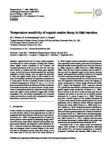
Figure 1-1. Amount of Ra precipitated as radiobarite after 2,700 y of repository release in the till domain (from Piqué et al. 2010).
Repository-derived Th is also readily sorbed onto illite. The decay of 230Th produces 226Ra, which, unlike Th and Cs, is not efficiently retained onto illite (Piqué et al. 2010). However, if the growth of Ba from Cs decay is high enough to reach barite saturation, the Ra released from Th decay could be partially retained in the newly formed barite, decreasing the 226Ra concentration that would reach the surface. Repository-derived nickel was also considered in the earlier simulations reported by Piqué et al. (2010); in this case, it was well retained in the near-surface system through sorption onto illite. Both 59Ni and 63Ni can contribute to the radioactive dose, and since 63Ni has a half-life of only 100.1 years, neglecting its decay can introduce uncertainties in the results. The degree of uncertainty will depend on several factors, such as the time at which the canister is breached as well as the 63Ni/NiT ratio.
1.2 Objectives The main objective of this work is to quantify the effect of coupling radioactive decay of selected radionuclides of Th, Ra, Ni and Cs with transport and retention of these radionuclides in the 2D model till model of Piqué et al. (2010). The study aims at evaluating the uncertainty in the results from the previous models and the role played by each geochemical process in the retention of radionuclides when decay is included. The model of the till has recently been updated (Johansson 2008). As a result, till parameterisation (the physical extent of layers characterised by different porosities and hydraulic conductivities) has changed resulting in a so called 2-layer till model, which is the current reference till model. As the updated 2-layer till model underpins the current state-of-the-art model for radionuclide transport, additional objectives of this work are to: • Assess the effect of changed till parameterisation on modelled groundwater flow and solute transport between the previous (3-layer) and the current (2-layer) till models. • Evaluate the effect of radioactive decay on the transport of 135Cs, 59Ni, 226Ra and 230Th in the current 2-layer till model. • Analyse sensitivities and estimate uncertainties associated with key parameters and assumptions through probabilistic and deterministic sensitivity calculations.
1.3 Methodology As a first step, the expected concentrations of selected radionuclides in the deep groundwater after release from the repository are estimated. To this end, the inventories of Th, Ni and Cs isotopes in the repository at the time of release are calculated and the isotope concentrations in the deep groundwater are evaluated based on equilibria with solubility-controlling phases.
8
SKB R-13-02
Batch calculations that consider radioactive decay of selected isotopes are performed using PHREEQC and AMBER. Benchmarking of the two codes is carried to test the correctness of implementation of radioactive decay in PHREEQC. Subsequently, radioactive decay and retention processes are coupled in batch calculations. The retention processes considered are the same as those in the previous study by Piqué et al. (2010). Probabilistic sensitivity analysis regarding the batch calculations is performed using MCPhreeqC – a tool that allows performing Monte Carlo simulations with PHREEQC. The results of this task feed into deterministic sensitivity calculations for the 2D reactive transport modelling. Next, radionuclide decay coupled with retention processes is implemented in 2D reactive transport models using PHAST. This task involves simulation of radionuclide release into the till domain for a period of 2,700 y. For this purpose numerical simulations performed within the previous project (Piqué et al. 2010) are revised and the decay chains are implemented. In addition, a deterministic sensitivity analysis of key geochemical parameters and processes is carried out. The reactive transport models of the till initially consider three layers with different hydraulic properties (the 3-layer till model). The hydrodynamic model is updated, following the 2-layer model of Johansson (2008). Results obtained for the 2-layer till model are compared with those obtained for the 3-layer model. Moreover, scoping calculations assessing the effect of organics on Ra transport are carried out. A detailed description of the methodology is presented in the chapters below.
SKB R-13-02 9
2
Implementation of coupled radioactive decay and retention processes in PHREEQC
The 2D reactive transport simulations described by Piqué et al. (2010) were carried out using the PHAST code (Parkhurst et al. 2004), which couples the transport code HST3D (Kipp 1997) and the geochemical simulator PHREEQC (Parkhurst and Appelo 1999). The 2D transport modelling in this project has also been performed using PHAST, where radionuclide decay and decay chains were implemented as kinetic reactions in PHREEQC. Correct implementation of radioactive decay was tested by a benchmarking study that compared results of batch simulations obtained using PHREEQC with those calculated using the AMBER code (Amber 2006). The following subsections provide details on the thermodynamic database, the groundwater types, the amount of each radionuclide assumed to be initially present in the groundwater, the implementation of radioactive decay, and the coupling of decay with different retention processes used/implemented in the calculations with PHREEQC.
2.1
Thermodynamic database
2.1.1 Modifications of SKB-TDB The SKB thermodynamic database (SKB-TDB) has been used in the calculations. This database was developed by Hummel et al. (2002) with modifications by Duro et al. (2006a). Several modifications, described below, were incorporated in the present modelling. Two Fe(III) carbonate species originally missing from the TDB were added (see Table 2-1). The speciation of Ba and the solubility constant of barite were updated (Table 2-1). Some lacking Ni species have been added (Table 2-1). Thermo dynamic data of all the species in Table 2-1 were taken from the SIT database, which was developed by Amphos21 for ANDRA (Duro et al. 2010) and corresponds to the PHREEQC version of the ThermoChimie v.7.b database, available in the 2.17 version of PHREEQC. 2.1.2 Addition of repository-derived radionuclides to the SKB-TDB The radionuclides of interest to follow after their release from the repository were labelled (e.g. 59Ni). 226 Ra was not labelled since, before repository release, its concentration in the studied groundwater is considered to be generally very low (below about 10–13 mol/L (SKB 2007)). Table 2-1. Equilibrium constants of complexation reactions for aqueous species and dissolution reactions for solid phases added to the SKB-TDB. Reaction
Log K (25°C)
Aqueous species Fe3+ + CO32– +H2O ↔ FeOHCO3 + H+
10.76
Fe3+ + 3 CO32– ↔ Fe(CO3)33–
24.24
Ba2+ + CO32– ↔ BaCO3
2.71
Ba2+ + SO42– ↔ BaSO4
2.70
Ba2+ + Cl– ↔ BaCl+ Ba2+ + H2O ↔ BaOH+ + H+ Ba2+ + CO32– + H+ ↔ BaHCO3+
0.06 –13.47 8.56
Ni2+ + S2O32– ↔ NiS2O3
2.06
Ni2+ + 2 HS– ↔ Ni(HS)2
11.10
Ni2+ + 2 CO32– ↔ Ni(CO3)22– Ni2+ + CO32– + H+ ↔ NiHCO3+ Ni2+ + 2 SO42– ↔ Ni(SO4)22–
6.20 11.73 3.01
Solid phases Barite: BaSO4 ↔ Ba2+ + SO42–
–9.97
SKB R-13-02 11
The labelling of repository-derived radionuclides involved the addition of the labelled species as primary species in the thermodynamic database. The secondary aqueous species and the reactions involving solid phases were added for the labelled radionuclides by duplicating the reactions of the non-labelled isotopes and replacing them with the labelled radionuclides. The total concentration of the selected element at any given time will be the sum of the non-labelled and the labelled species. In order to involve repository-derived radionuclides and the naturally occurring isotopes in the same solid phase without causing isotopic fractionation, new solid solutions that involve both species have been added to the thermodynamic database. For more details see Piqué et al. (2010, Section 5.5.5).
2.2
Selection of the reference groundwater for modelling
2.2.1 Groundwater compositions The groundwater selected for the batch simulations is the deep groundwater used in the previous calculations of Piqué et al. (2010). The selected groundwater was sampled at a depth of 316 m at the KFM01D borehole. It is of Na-Cl type with a moderate salinity (ionic strength of 0.13 M). The composition of the reference groundwater results from the equilibrium of the water sampled in the borehole KFM01D with pyrite and calcite, which are the pure phases expected to control the Eh and pH, respectively. Chloride was used to ensure the electroneutrality of the solution. Groundwater chemistry is reported in Table 2-1 (note that this is the composition of the groundwater before the expected release of radio nuclides from the repository). Under these conditions U is represented mainly by uranyl-carbonate complexes, while the most abundant uranious species are U(IV)-hydroxides (whose concentrations are about an order of magnitude lower than those of the uranyl-carbonate complexes). Hydroxy-complexes are also the main Th species. The speciation of Fe is dominated by ferrous iron (mainly Fe2+), while the most abundant ferric iron species (Fe-hydrocarbonate) is about five orders of magnitude lower in concentration. The measured concentrations of Ba and U were 2.14∙10–6 and 2∙10–8 mol/L, respectively (Laaksoharju et al. 2008). Using these values and assuming equilibrium with calcite and pyrite as the Eh-controlling phase, the groundwater was calculated to be supersaturated with respect to barite (SI = 0.64) and amorphous uraninite (SI = 0.25). As these minerals are expected to be in equilibrium with the deep groundwater and may play a major role in the retention of Ba and U, it was decided to reduce the concentrations of dissolved Ba and U in the groundwater so as to avoid supersaturation. The concentration of Ba was decreased to 4.85∙10–7 mol/L, while that of U was decreased to 1.11∙10–8 mol/L (Table 2-2). The calculated supersaturation could be due to a number of reasons, including presence of a mineral in the form of small crystals (increased solubility), presence of solid-solutions (e.g.: (Ba,Sr) SO4) rather than pure phases, or presence of an agent inhibiting mineral precipitation. The chemical composition of the till groundwater is taken from Piqué et al. (2010), where a detailed description of the expected geochemical conditions is presented. This groundwater composition was calculated by equilibrating a solution representing the sample taken in soil pipe SFM0002 with (Ca,Sr)CO3 solid solution, siderite and ferrihydrite. As this water was close to equilibrium with these minerals, the resulting composition did not change much after equilibration. The iron concentration was slightly modified by the equilibrium with ferrihydrite, and strontium by the equilibrium with the solid solution. The redox state of the solution was controlled by the Fe2+/ferrihydrite pair, and the pH by the equilibrium with the (Ca,Sr)CO3 solid solution and siderite. Under these conditions, uranium is found as U(VI) and the dominant aqueous species are carbonate complexes, mainly UO2(CO3)34–. All uranium solid phases are far from saturation. Thorium, similarly to U(VI), is found mainly as carbonate complexes in solution, predominantly Th(OH)3CO3– and Th(OH)2(CO3)22–. All Th solid phases are far from saturation. The speciation of iron is dominanted by Fe(II), mainly Fe2+, while the most abundant Fe(III) species (Fe(II)-hydroxy-carbonate) is about four orders of magnitude lower in concentration. The chemical composition of the till groundwater is presented in Table 2-3.
12
SKB R-13-02
Table 2-2. Chemical composition of the reference groundwater (before radionuclide release from the repository) used in the numerical calculations (modified after Laaksoharju et al. 2008). In boldface are indicated Ba and U whose concentrations were decreased in order to avoid oversaturation with respect to barite and amorphous uraninite, respectively (see explanation in the text). Parameter
Reference Groundwater mol/L
pH Eh (V) [Na]total [K]total [Ca]total [Mg]total [Sr]total [Ba]total [C]total [Cl]total [S]total [Si]total [Fe]total [NH4+] DOC [U]total [Cs]total [Ni]total [Th]total
mg/L
6.78 –0.152 6.13·10–2 2.67 7.98·10–4 2.04∙10–2 –2 1.82·10 4.54∙10–1 4.73·10–3 1.95∙10–1 6.94·10–5 7.92∙10–4 4.85·10–7
3.53∙10–6
4.72·10 1.00·10–1 2.21·10–3 5.63·10–4 5.78·10–5 7.28·10–5 6.66·10–4
3.93∙10–1 2.82 3.45∙10–2 2.00∙10–2 1.03∙10–3 4.04∙10–3 5.55∙10–2
1.11·10–8
4.66∙10–8
3.65·10–9 7.17·10–9 1.19·10–9
2.75∙10–8 1.22∙10–7 5.13∙10–9
–3
Table 2-3. Chemical composition of the till groundwater used in the numerical calculations. Parameter
Till groundwater mol/L mg/L
pH Eh (V) [Na]total [K]total [Ca]total [Mg]total [Sr]total [Ba]total [C]total [Cl]total [S]total [Fe]total [NH4+] [U]total [Cs]total [Ni]total [Th]total [P]total
7.12 0.003 1.22·10–3 5.31·10–2 –4 1.22·10 3.12·10–3 2.79·10–3 6.97·10–2 3.54·10–4 1.46·10–2 –6 2.10·10 2.40·10–5 –7 7.28·10 5.30·10–6 5.58·10–3 4.65·10–1 –3 1.90·10 5.36·10–2 –4 2.21·10 3.76·10–3 1.75·10–5 3.13·10–4 6.62·10–6 3.67·10–4 –8 2.24·10 9.41·10–8 –11 6.48·10 4.87·10–10 4.42·10–8 7.52·10–7 6.09·10–10 2.63·10–9 1.29·10–6 4.16·10–5
2.2.2 Solubility limits of selected elements in groundwater The repository-derived radionuclides of interest in this project are those of U, Th, Ra, Ni and Cs. In Piqué et al. (2010) the initial concentration of repository-derived nuclides in solution was set according to a very pessimistic assumption according to which the geosphere has no retention capacity for the radionuclides and radionuclide transport from the repository to the near-surface systems is instantaneous. In this context, the concentrations of dissolved U, Th and Ni after repository-release are calculated assuming equilibrium of the reference groundwater with their solubility-limiting phases in the near-field.
SKB R-13-02 13
Piqué et al. (2010) considered UO2·2H2O(am), ThO2·2H2O(am) and millerite (NiS) as the solubilitylimiting phases. Note that the solubility limit applies to the total amount of the element of interest, i.e. it corresponds to the sum of natural and repository-derived isotopes. The solubility limits for U and Ni in the reference deep groundwater are consistent with the mean concentrations measured in Forsmark deep groundwater. However, the solubility limit of Th is more than two orders of magnitude above the mean concentration of dissolved Th measured in groundwater. For ThO2·2H2O(am), two solubility constants are suggested in the NEA-TDB (Rand et al. 2008); they distinguish between fresh and aged Th(IV) hydroxide or hydrous oxide (Table 2-4). In the modelling reported by Piqué et al. (2010), ThO2·2H2O(am, fresh) was selected as the solubility-limiting phase, following Duro et al. (2006b). However, Rand et al. (2008) recommend ThO2·2H2O(am, aged) for modelling thorium solubilities in natural systems. Applying the solubility constant of ThO2·2H2O(am, aged), the solubility of Th in the reference groundwater is lowered one order of magnitude, being thus closer to the measured concentrations of natural Th in solution. For this reason, ThO2·2H2O(am, aged) has been selected as the solubility-limiting phase in this project. The solubility limits to be used are reported in Table 2-5. As the solubility limiting phases for Ra and Cs in the near-field are difficult to identify, radioactive release estimated at the near-field were used to constrain their concentrations (Piqué et al. 2010). The concentration of 135Cs is 3.48·10–7 mol/L and that of 226Ra is 9.15·10–11 mol/L.
2.2.3 Amount of selected repository-derived radionuclides in groundwater The maximum amount of repository-derived Th and Ni in the reference groundwater is calculated by subtracting the concentration of natural Th and Ni from the solubility limit (Table 2-6). The resulting concentrations are close to the solubility limit, since those of natural thorium and nickel are far from saturation and hence do not reduce the concentrations much (see Table 2-2 and Table 2-5). The values reported in Table 2-6 correspond to the sum of isotopes of each element theoretically released from the waste; the next step is defining the relative proportion of each radioisotope of Th and of Ni at different times. This is done by assuming that the spent fuel dissolves congruently and by calculating the evolution of the radionuclide inventory in the repository with time. A 10,000 years evolution was calculated with the code AMBER, version 5.1. The inventory used was that recommended for use in the SR-Site (SKB 2010a). This inventory is partially reproduced in Table 2-7 (only the radionuclides involved in the calculations are reported). For most radionuclides the UO2 spent fuel is the dominating source, while for 59Ni and 63Ni, the total inventory is significantly affected by the inventory of the construction material, crud, or control rods (SKB 2010b). Table 2-4. Solubility constants of ThO2(am, hyd) (Rand et al. 2008). Phase
Reaction
Log K (25°C)
ThO2·2H2O(am, fresh)
ThO2·2H2O +4 H+ ↔ Th4+ + 4 H2O
9.3 ± 0.9
ThO2·2H2O(am, aged)
ThO2·2H2O +4 H+ ↔ Th4+ + 4 H2O
8.5 ± 0.9
Table 2-5. Solubility limits of U, Th and Ni in the reference groundwater and solubility-limiting phases used in this work. Element mol/L
Solubility limit mg/L
Solubility-limiting phase
[U]total
1.11∙10–8
2.64∙10–3
UO2·2H2O(am)
[Th]total
2.12∙10
–8
4.92∙10–3
ThO2·2H2O(am, aged)
[Ni]total
3.64∙10–7
2.14∙10–2
Millerite
14
SKB R-13-02
Table 2-6. Maximum concentration of repository-derived Th and Ni in the reference groundwater (GW). Element mol/L
Reference GW mg/L
[Th]repository-derived
2.00∙10–8
4.64∙10–3
[Ni]repository-derived
3.57∙10
2.10∙10–2
–7
The inventory includes all Th isotopes present in the spent fuel in significant amount at the year 2045, namely 229Th, 230Th, 232Th and 234Th. Also, parent nuclides have been included in the calculations, to reproduce the evolution of Th budget in the fuel with time. 230Th and 234Th belong to the 238U decay chain, 232Th to the 240Pu decay chain and 229Th belongs to the 241Pu decay chain. Other Th isotopes that will be produced as decay products in the spent fuel (227Th, 228Th, and 231Th) have not been included in the calculations, since their concentrations are not expected to be significant. The amount of 232Th, 230Th and 229Th in a fuel canister increases by several orders of magnitude with time, while that of 234Th is maintained constant (Figure 2-1). Most of the Th budget in the fuel corresponds to 230Th (between 77% and 82%), followed by 232Th (19–20%), and in much lesser amount 229 Th (≤ 1.2%). Therefore, it has been approximated that the 80% of repository-derived Th in the reference groundwater corresponds to 230Th and the remaining 20% to 232Th, at any time after the canister failure (234Th and 229Th have been neglected). Since the half-live of 232Th is 1.4×10¹⁰ y, it is considered to behave as a stable isotope over the calculation time span (2,700 y) and has not been labelled, while radioactive decay has been simulated for 230Th (labelled). All natural Th is considered to be 232Th. Most of Ni derives from construction materials (e.g. cladding, fuel channel). The content of Ni in the construction material is of 1.99 and 2.46 kg for typical BWR and PWR fuel assemblies, respectively (SKB 2010b). Considering that 47,904 BWR fuel assemblies and 6,049 PWR fuel assemblies will be deposited in a total number of 6,103 canisters (SKB 2010b), the total amount of Ni in the fuel assembly per average canister is 18.06 kg. Accordingly, from the radionuclide inventory (Table 2-7) the relative proportions of 59Ni and 63Ni over total Ni per average canister can be derived. Most of the nickel inventory in the canister corresponds to stable nickel isotopes; at the year 2045, the proportions of 59Ni/NiT and 63Ni/NiT are 0.52% and 0.074%, respectively. Table 2-7. Selected inventory in moles per average fuel canister at year 2,045 based on a total number of 6,103 canisters (SKB 2010a). Radionuclide
Amount per average canister [mol/canister] Notes
Americium-241
9.21
Pu-241 decay chain
Caesium-135
6.73
Fission product
Caesium-137
8.69
Fission product
Neptunium-237
4.71
Pu-241 decay chain
Nickel-59
1.61
Activation product
Nickel-63
2.29∙10–1
Activation product
Plutonium-240
2.0∙101
Plutonium-241
1.86
Protactinium-233
1.63∙10–7
Pu-241 decay chain
Protactinium-234 m
3.67∙10–12
U-238 decay chain
Thorium-229
1.46∙10–8
Pu-241 decay chain
Thorium-230
1.75∙10–4
U-238 decay chain
Thorium-232
4.49∙10–5
Pu-240 decay chain
Thorium-234
1.07∙10–7
U-238 decay chain
Uranium-233
9.53∙10–5
Pu-241 decay chain
Uranium-234
1.82
U-238 decay chain
Uranium-236
3.91∙101
Pu-240 decay chain
Uranium-238
7.20∙103
SKB R-13-02 15
Since 59Ni and 63Ni are activation products, it is assumed that they are no longer produced once the fuel assembly is in the repository, and only decay is simulated. The amount of 63Ni quickly decreases with time, while the longer half-life of 59Ni results in limited loss of this radionuclide (Figure 2-2). Consequently, the proportion of 59Ni/NiT is almost constant, ranging between 0.52 and 0.48% over 10,000 years. Due to this small range, the value of 0.5% has been selected to calculate the initial amount of 59Ni in the reference groundwater. The proportion of 63Ni/NiT is below 0.001% after 300 years, for which reason this radionuclide has not been implemented in the calculations. The spent fuel contains two radioactive isotopes of Cs, 137Cs and 135Cs. Both are fission products of the nuclear reactor. The evolution with time of 137Cs and 135Cs concentrations in the average canister has been calculated (Figure 2-3), assuming that natural fission in the repository would not take place (or would be insignificant). The amount of 135Cs shows limited decrease over 10,000 years of simulation, due to its long half-life (2.30·106 years). On the other hand, the amount of 137Cs decreases significantly; after 500 years, the proportion of Cs/(137Cs+135Cs) is below 0.001%, therefore, this radionuclide has not been implemented in the simulations (it has been considered that repository failure would not take place before 500 years of storage). Since a solubility-limiting phase in the near field has not been defined for caesium, the amount of repository-derived 135Cs in the reference groundwater has been taken from Piqué et al. (2010), who used the radioactive release dose estimated at the near-field. The concentration of 135Cs in the reference groundwater after repository failure would be 3.48·10–7 mol/L. 137
For radium, the radioactive release dose was also taken into account to calculate the concentration of 226Ra in the reference groundwater after release from repository. In this case the concentration of dissolved 226Ra would be 9.15·10–11 mol/L. The composition of the reference groundwater after repository failure is reported in Table 2-8. 1E-1
90
Th-230 Th-232
80
1E-2
Th-234
60 1E-4
50 40
1E-5
30 1E-6
Th-229
Th isotope/ total Th (%)
Th (mol/average canister)
70 1E-3
Th-230 (%) Th-232 (%) Th-234 (%) Th-229 (%)
20 1E-7
10
1E-8 1
10
100
1000
0 10000
time (y)
Figure 2-1. Evolution of the inventory of thorium in the average canister. Year 1 corresponds to year 2,046. Calculations made with AMBER.
16
SKB R-13-02
1E+3
0,9
1E+1
0,8
1E-1
0,7
1E-3
0,6
1E-5
0,5
1E-7
0,4
1E-9
0,3
1E-11
0,2
1E-13
0,1
Ni stable
1E-15 1
10
100
1000
Ni-63 Ni-59 (%) Ni-63 (%)
Ni isotope/ total Ni (%)
Ni (mol/average canister)
Ni-59
0 10000
time (y)
Figure 2-2. Evolution of the inventory of nickel in the average canister. Year 1 corresponds to year 2,046. Calculations made with AMBER. 100 1E+1
80
1E-3
70
1E-5
60 50
1E-7
40 1E-9 30 1E-11
20
1E-13
Cs-137
Cs isotope/ (Cs-135 + Cs-137) (%)
1E-1
Cs (mol/average canister)
Cs-135
90
Cs-137 (%) Cs-135 (%)
10
1E-15 1
10
100
1000
0 10000
time (y)
Figure 2-3. Evolution of the inventory of radioactive caesium in the average canister. Year 1 corresponds to year 2,046. Calculations made with AMBER.
SKB R-13-02 17
Table 2-8. Approximate composition of the Reference GroundWater (RGW) after radionuclide release from the repository. Parameter
RGW mg/L
mol/L pH
Remarks
6.78
pe
–2.58
–2.58
[Na]total
6.13·10–2
2.67
[K]total
7.98·10–4
2.04∙10–2
[Ca]total
1.82·10
–2
4.54∙10–1
[Mg]total
4.73·10
–3
1.95∙10–1
[Sr]total
6.94·10
–5
7.92∙10–4
[Ba]total
4.85·10
–7
3.53∙10–6
[C]total
4.72·10
–3
3.93∙10–1
[Cl]total
1.00·10
–1
2.82
[S]total
2.21·10–3
3.45∙10–2
[Si]total
5.63·10
–4
2.00∙10–2
[Fe]total
5.78·10
–5
1.03∙10–3
+
[NH4 ]
7.28·10
–5
4.04∙10–3
DOC
6.66·10
–4
5.55∙10–2
[U]total
1.11·10
–8
4.66∙10–8
Natural + repository-derived isotopes
[Cs]total
3.65·10
–9
2.75∙10–8
Natural isotopes
[Ni]total
3.62·10–7
6.17∙10–6
Natural + repository-derived stable isotopes
[Th]total
5.20·10–9
2.24∙10–8
Natural + repository-derived 232Th
2.58∙10
–6
Repository-derived
[ Cs]total
3.48·10
[59Ni]total
1.79·10–9
3.03∙10–8
Repository-derived
[230Th]total
1.60·10–8
6.96∙10–8
Repository-derived
[226Ra]total
9.1·×10–11
4.03∙10–10
Repository-derived
135
2.3
–7
Implementation of radioactive decay and decay chains in PHREEQC
2.3.1 Identification and description of decay chains Preliminary calculations using the AMBER code were carried out in order to evaluate the relative importance of decay dynamics for several radionuclides of U and Th present in the spent fuel (Figure 2-4). The results indicate that over a period of time relevant for the reactive transport calculations (2,700 years) 238U and 234U are sufficiently long-lived that their decay can be ignored in the calculations with no practical impact on the results. Therefore, the implementation of the 238U decay chain starts with the radionuclide of 230Th, which has the added advantage of simplifying the amount of necessary calculations. As the only radionuclides included in the chain are 230Th and 226Ra, U isotopes were not labelled. Radionuclide decay was programmed in the PHREEQC code using the KINETICS and RATE keywords. The following decay or decay chains have been implemented in PHREEQC: Th → 226Ra → 222Rn
230
Cs → 135Ba
135
Ni → 59Co
59
Only the isotopes denoted in bold font were quantified in the simulations. Half-lives used have been taken from Table C-1 of the Spent fuel report (SKB 2010b). Note that 135Ba and 59Co are stable. In order to verify that radionuclide decay was implemented correctly, results obtained using the PHREEQC model were benchmarked against calculations carried out using the AMBER code. The PHREEQC simulations were run up to 3,000 years, divided in time steps of 10 years. The same calculations were carried out increasing the time steps to 20 and 50 years in order to assess sensitivity. 18
SKB R-13-02
1.0E-02
U-238
Concentration (mol/g U)
1.0E-03
U-234
1.0E-04
U-235
1.0E-05
U-236
1.0E-06
U-233
1.0E-07
Th-230
1.0E-08
Th-232
1.0E-09
Th-229
1.0E-10 1.0E-11 1.0E-12 1.0E-13 1.0E-14 10
100
1000
10000
100000
Time (y)
Figure 2-4. Evolution dynamics of concentrations of selected U and Th radionuclides in the spent nuclear fuel (ATM-104) over a period of 100,000 years due to radioactive decay. Results calculated with the AMBER code.
The calculated concentrations of 230Th, 135Cs, 135Ba and 59Ni are identical in the three PHREEQC batch simulations (time steps of 10, 20 and 50 years). The calculations performed with AMBER gave identical results, with only minor (on the 4th decimal place) differences in some cases. With respect to 226Ra, the calculation is more complex since it involves coupled growth and decay. In this case the results show slight deviations for different time steps, in particular for the run with a time step of 50 years (Table 2-9).
2.3.2 Coupling geochemical processes and radioactive decay Previous reactive transport models (Grandia et al. 2007, Sena et al. 2008, Piqué et al. 2010) have shown that the near-surface systems constitute geochemically reactive barriers able to retain radionuclides by several key processes. For the specific case of U, Th, Ra, Ni and Cs, a number of geochemical processes can be involved in their retention in the Forsmark till). The geochemical processes implemented in the numerical simulations have been summarised in the following paragraphs – Table 2-10 (for details, see Piqué et al. 2010). Table 2-9. Comparison of PHREEQC batch simulations and AMBER calculations for 226Ra in the reference groundwater (mol/L). Incremental time steps of: (1) 10 years – Base Case, (2) 20 years, (3) 50 years used. PHC – PHREEQC, y – year, ret. – retention, Δ% – percent difference with respect to the Base Case. Time [y]
PHC1 (decay only)
Δ%PHC2 (decay only)
Δ%PHC3 (decay only)
Δ%AMBER (decay only)
PHC1 (decay+ret.)
Δ%PHC2 (decay+ret.)
100
1.446·10–11
0.17
0.56
0.15
1.446·10–11
0.17
200
2.819·10
–11
0.19
0.70
0.16
2.819·10–11
0.19
300
4.133·10–11
0.20
0.74
0.19
4.133·10–11
0.20
400
5.390·10–11
0.19
0.75
0.19
5.390·10–11
0.19
500
6.592·10–11
0.19
0.75
0.20
6.592·10–11
0.19
1000
1.186·10–10
0.18
0.69
0.18
1.186·10–10
0.18
1500
1.607·10–10
0.16
0.62
0.26
1.607·10–10
0.16
2000
1.943·10–10
0.14
0.56
0.28
1.943·10–10
0.14
2500
2.210·10–10
0.12
0.49
0.29
2.210·10–10
0.12
3000
2.422·10–10
0.11
0.43
0.30
2.422·10–10
0.11
SKB R-13-02 19
Table 2-10. Retention processes implemented (marked with a cross) in the numerical simulations for the radionuclides of interest. Retention Process
230
Sorption onto Fe-oxyhydroxides Sorption onto Phyllosilicates Precipitation as a pure phase Co-precipitation with sulphates
× ×
Th
226
×
Ra
135
×
Cs
59
× ×
Ni
U × × ×
×
Sorption onto ferrihydrite: The surface complexation model of Waite et al. (1994) was implemented. Adsorbing carbonate species were also included in the simulations. The sorption constants for Ni2+ are those from Dzombak and Morel (1990). Ferrihydrite is a reactive mineral very sensitive to changes in the redox state of the system. For this reason, the total amount of sites available for adsorption depends on the amount of ferrihydrite present at each time step of the calculation. Sorption onto illite: Bradbury and Baeyens (2009a, b) quantitatively described the sorption of U, Th and Ni (among other elements) onto Na-illite by means of surface complexation and cationexchange. Three types of surface complexation sites were considered, one strong site and two amphoteric edge sites. Metal uptake was modelled to occur on strong-type sites only. The three-site cation-exchange model of Bradbury and Baeyens (2000) was implemented. 80% of the sites are of planar type, which can exchange either divalent or monovalent cations. Type II (20% of sites) and Frayed Edge Sites (FES; 0.25% of sites), involve monovalent species such as Na+, K+, Cs+ and NH4+. An illite amount of 10 wt% in the till was considered in the calculations (approximate value based on data from Hedenström (2004) and Lindborg (2008)). The specific surface area and site density were taken from Bradbury and Baeyens (2009a). Thermodynamic data for sorption of U, Th and Ni were taken from Bradbury and Baeyens (2009a, b). A cation exchange capacity of 225 meq/kg was considered (Baeyens and Bradbury 2004). Cation-exchange selectivity coefficients consistent with the Gaines-Thomas convention are the same as those used by Piqué et al. (2010). Precipitation of ThO2·2H2O: To retain repository-derived 230Th and the non-labelled Th isotopes in the same solid phase without causing isotopic fractionation, a solid solution that involves both species was added to the thermodynamic database. The mineral phase considered as a sink for Th was amorp hous thorianite. The dissolution reaction of this mineral phase (Equation 2‑1) was replaced by an ideal solid solution (Equation 2‑2): 2‑2 ThO2·2H2O+4H + ↔Th4++4H2O Equation 2‑3 (Th1–χ RDThχ)O2·2H2O+4H +↔(1–χ)Th4++χRDTh4++4H2O Equation where χ is the molar fraction of repository-derived 230Th (RDTh) in amorphous thorianite. Incorporation of 226Ra in barite: A binary solid solution with BaSO4 and RaSO4 as end-members was implemented in the simulations. The solid solution was considered to be ideal. Only very small fractions of RaSO4 are expected to be incorporated due to the low radium concentration (in the order of 10–11 mol/L) compared with barium. The above-described retention processes were coupled with radioactive decay in PHREEQC. The implementation of the different retention processes was done one by one, and tested in batch simulations. The simulations with coupled decay and retention processes gave the same results for total 230Th, 59Ni and 135Cs as the simulation of decay only (not shown), using both the 10-year and 20-year time-steps. In order to minimise possible discrepancies arising in the calculations, the shorter time step (10 years) was used.
20
SKB R-13-02
2.4
Role of organic complexation in 226Ra transport
In near-surface environments, the behaviour of Ra is influenced by complexation with inorganic and organic ligands, incorporation into secondary phases and adsorption onto clay minerals and solid organic matter. Sorption onto solid organic phases can play a role in the retention of Ra in soils (IAEA 1984). Complexation of Ra with dissolved organic matter is not well known. Due to affinity of Ra2+ for solid organic matter, it is expected that Ra2+ will also form complexes with dissolved organic acids. Within the present project, a literature search for thermodynamic data on Ra-organic complexes was performed. The outcome indicated that available data were scarce. However, formation constants for Ra-acetate complexes can be estimated based on existing data for analogue alkaline earth elements. These Ra-acetate complexes have been implemented in the thermodynamic database to assess the effects on the speciation of aqueous Ra. In addition, Ca-acetate complexes have been also implemented in order to simulate competition for the acetate ligand. The Ra-acetate complexes implemented and their thermodynamic constants are shown in Table 2-11. Speciation calculations were carried out with the reference deep groundwater and the till porewater; an arbitrary concentration of 0.01 mol/L of acetate was added to both. The amount of 226Ra was set to 1·10–10 mol/L. The results show that for both the deep groundwater and till porewater, the dominant species is Ra2+ (Figure 2-5). The second most abundant species is RaSO4(aq), whose concentration is one order of magnitude lower than Ra2+ in the till porewater and of almost one order in the deep groundwater. Of the two Ra-acetate species, Ra-Acetate+ is the dominant in both cases. In the deep groundwater it represents a concentration which is one order and a half lower than the dominant species (Ra2+), and in the till porewater the concentration of Ra-Acetate+ is one order of magnitude below that of Ra2+ (Figure 2-5). Given the above results on Ra speciation calculations, and given that the amount of acetate used in the calculations was very high (more realistic, lower acetate values would result in a lower proportion of Ra-acetate species), the role of acetate complexation for Ra transport was considered insignificant and the process has not been implemented in the reactive transport simulations. Table 2-11. Equilibrium constants for the complexation of Ra with acetate. Reaction
Log K (25°C)
Ra + CH3COO = Ra(CH3COO)
1.048
Ra2+ + 2 CH3COO– = Ra(CH3COO)2
1.613
2+
–
+
SKB R-13-02 21
A
Log concentration (mol/L)
-10
-11
Ra+2 RaAcetate+ RaAcetate2
-12
RaCO3(aq) RaHCO3+ RaOH+
-13
RaSO4(aq) RaCl+ RaCl2(aq)
-14
-15
4
5
6
7
8
9
10
11
12
pH
B
Log concentration (mol/L)
-10
-11
Ra +2 RaAcetate+ RaAcetate2
-12
RaCO3(aq) RaHCO3+ RaOH+
-13
RaSO4(aq) RaCl+
-14
-15
4
5
6
7
8
9
10
11
12
pH
Figure 2-5. Speciation of Ra in the deep groundwater (A) and the till porewater (B). Acetate concentration is 0.01 mol/L. Total Ra concentration is 1·10–10 mol/L.
22
SKB R-13-02
3
Probabilistic sensitivity analysis
Over the last decades efforts have been made to simulate reactive transport of radionuclides in porous media. Most of these models rely on a “classical” deterministic description of the problem while the analysis of the uncertainty is left to few sensitivity runs with minimum, maximum and average values for specific parameters. An alternative and more robust approach to deal with uncertainty is to apply stochastic modelling using Monte-Carlo simulations. In this work, Monte-Carlo simulations were performed using the numerical tool MCPhreeqc, developed by Amphos21. In MCPhreeqC input for a stochastic simulation is entered through a userfriendly graphical interface. Based on available data and/or expert judgment, a probability density function (PDF) is defined for each parameter considered in the simulation. The framework executes the PHREEQC code multiple times (10,000 realisation in this case) while parameter values are sampled randomly from a cumulative probability function (calculated from the PDF). The combined output of these runs provides information about uncertainty for specific output variables resulting from the uncertainty of the input parameters.
3.1
Modelling setup
For the Monte-Carlo analysis, batch tests were run with PHREEQC. These tests simulate the inter action of the deep groundwater with the Quaternary till. Decay chains were not implemented in these calculations. The batch simulations were run in two steps: 1) equilibration of illite and ferrihydrite sorption sites with radionuclide-free deep groundwater; and 2) interaction of the equilibrated surfaces with the same groundwater, which also carries repository-derived nuclides.
3.2
Selection of parameters for probabilistic analysis
The main geochemical parameters that can play a role in the retention of each radioelement under study are summarised below (Table 3-1). Major elements in groundwater are not independent variables, but are correlated with each other, either due to mineralogical control or groundwater mixing (or both). The groundwater pH and redox potential are also controlled by equilibrium with solid phases. Therefore, conditional probability distribution functions need to be implemented for these parameters. In this particular case it was decided to evaluate groundwater types using a deterministic approach. Three water types or “end-members” were selected for this statistical study, which are found at the emplacement depth of the future HLNW repository. The composition on the selected groundwater end-members is shown in Table 3-2. The pH was fixed to be in equilibrium with calcite. The same analysis was done for the reference groundwater. Trace elements and solid phases were simulated as stochastic variables. In order to distinguish the effect of each parameter on the retention of radionuclides the parameters were tested in a sequence, one-by-one. Therefore, as many simulations as stochastic variables were run, plus one simulation that combines all the stochastic variables. In the simulations with one PDF, the other parameters were fixed (see concentrations shown in Table 3-3).
SKB R-13-02 23
Table 3-1. Main geochemical parameters (marked with a cross) that can have an effect on radionuclide retention in the Forsmark till domain. ppt – precipitation. HFO – hydrous ferric oxides. Parameter
226
Radiobarite ppt
S(VI)aq C(IV)aq Naaq Kaq Mgaq Caaq Sraq Baaq NH4aq Feaq Uaq Csaq Thaq Niaq Raaq 135 Csaq 230 Thaq 59 Niaq pH Eh % illite in till % HFO in till
× × ×
Ra Sorption on illite
× × × × × × × ×
× × ×
×
×
×
135 Cs Sorption on illite
230 Th Thorianite Sorption on ppt illite
Sorption on illite
× × × × × × × × ×
× ×
× ×
× ×
× ×
×
×
×
×
×
×
× ×
×
× ×
× ×
×
×
× × ×
× × ×
×
×
×
× ×
× ×
59
Ni Sorption on HFO
× × × ×
Table 3-2. Composition of major parameters in the three deep groundwater types considered as end-members in Monte Carlo calculations. Parameter
Brackish non-marine
Littorina
Transition
Ionic Strength pH Eh (V) Ca mol/L Mg mol/L Na mol/L K mol/L Sr mol/L Cl mol/L C mol/L S mol/L Fe mol/L
0.2624 8.02 –0.207 6.24·10–2 1.59·10–4 7.35·10–2 1.73·10–4 3.05·10–4 2.00·10–1 9.38·10–5 3.70·10–4 6.73·10–7
0.2014 7.05 –0.171 2.52·10–2 9.96·10–3 9.96·10–2 9.28·10–4 9.86·10–5 1.55·10–1 2.07·10–3 4.82·10–3 3.10·10–5
0.2019 7.57 –0.207 3.82·10–2 2.58·10–3 7.57·10–2 4.27·10–4 1.87·10–4 1.62·10–1 3.70·10–4 2.05·10–3 1.16·10–5
Table 3-3. Fixed concentrations of trace elements and solid phases used in Monte Carlo calculations (while testing the effect of a single parameter value). Parameter
Brackish non-marine
Littorina
Transition
Reference
Baaq mol/L NH4+aq mol/L U mol/L Cs mol/L Th mol/L Ni mol/L Ra mol/L RD Cs mol/L RD Th mol/L RD Ni mol/L Illite till wt% HFO till wt%
5.07·10 2.50·10–5 7.10·10–10 5.61·10–9 1.00·10–10 7.84·10–9 9.15·10–11 3.48·10–7 1.40·10–9 7.50·10–8 10 0.1
3.22·10 1.57·10–4 3.25·10–9 1.79·10–8 1.00·10–10 1.67·10–8 9.15·10–11 3.48·10–7 8.27·10–9 1.50·10–7 10 0.1
7.39·10 5.79·10–5 7.34·10–10 2.33·10–8 1.00·10–10 1.91·10–8 9.15·10–11 3.48·10–7 2.21·10–9 1.91·10–8 10 0.1
4.85·10–7 7.28·10–5 1.11·10–8 3.65·10–9 5.20·10–9 3.62·10–7 9.15·10–11 3.48·10–7 1.60·10–8 1.79·10–9 10 0.1
24
–6
–7
–7
SKB R-13-02
3.3
Construction of probabilistic distribution functions
The PDF of each variable was constructed using measured data; for the dissolved trace elements data from the KFM and HFM boreholes was used. Groundwaters sampled at these boreholes represent waters that could eventually interact with the repository. Most of the histograms of the measured data show extended tailing at the higher end concentration values. For data presentation reasons, it was therefore decided to apply a natural log transformation to the data. The log-transformed data were represented as Gaussian-shaped histograms to which natural log-normal PDFs were fitted (Figure 3-1). The PDF of Cs was truncated to avoid unrealistic values above solubility limits. In the case of Ni, the histogram after log-normal transformation still showed a tailing; therefore a gamma distribution was fitted to the values (Figure 3-2). To ensure positive values the natural log normal values were translated by 19.55.
Relative Frequency
Relative Frequency
A constraint for the maximum concentration of dissolved Ba exists; the groundwater cannot be oversaturated with barite. Accordingly, the PDF of Ba was truncated (Figure 3-3), and the maximum concentration corresponds to the solubility limit of barite for each groundwater type (Table 3-4). The fact that many Forsmark groundwaters have higher dissolved Ba than the calculated solubility limits can be explained by the fact that these groundwaters have a much lower amount of dissolved sulphate, thus allowing more barium to remain dissolved in solution (Figure 3-4).
ln(Cs) [mol/kgw]
Relative Frequency
Relative Frequency
ln(U) [mol/kgw]
ln(Ra) [mol/kgw]
ln(NH4 ) [mol/kgw]
Figure 3-1. Histograms of measured data and fitted PDFs for U, Cs, NH4 and Ra. The cut-off values for NH4, Cs and Ra are 1.67∙10–4 mol/L, 1.50∙10–6 mol/L and 9.15∙10–11 mol/L, respectively.
SKB R-13-02 25
Relative Frequency
ln(Ni) [mol/kgw]
Relative Frequency
Relative Frequency
Figure 3-2. Histogram of measured data and fitted PDF for Ni. The natural log normal values are translated by 19.55 to generate positive values.
ln(Ba) [mol/kgw]
Relative Frequency
Relative Frequency
ln(Ba) [mol/kgw]
ln(Ba) [mol/kgw]
ln(Ba) [mol/kgw]
Figure 3-3. Histogram of measured data and fitted PDFs for Ba, with different cut-offs for different waters (upper-left: Brackish Non-Marine, upper-right: Littorina, lower-left: Transition, lower-right: Reference). Table 3-4. Maximum concentration of dissolved Ba in each groundwater type. Parameter
Brackish non-marine Littorina
Transition
Reference
Baaq mol/L
5.07·10
7.39·10
4.85·10–7
26
–6
3.22·10
–7
–7
SKB R-13-02
3.00E+03
2.50E+03
[Ba] (ug/L)
2.00E+03
1.50E+03
1.00E+03
5.00E+02
0.00E+00 0.0E+00 1.0E+05 2.0E+05 3.0E+05 4.0E+05 5.0E+05 6.0E+05 7.0E+05 8.0E+05
[SO4] (ug/L)
Figure 3-4. Plot of dissolved sulphate versus barium measured in the HFM and KFM Forsmark boreholes. Table 3-5. Maximum and minimum concentration (in mol/L) of dissolved RD-Cs, RD-Th and RD-Ni for defining the uniform PDF. Brackish n-marine Parameter
Max
RD-Cs
Min
3.5·10
–07
RD-Ni
7.5·10
–08
RD-Th
1.4·10–09
Littorina Max
5.5·10
–11
1.0·10
–11
1.0·10–11
Transition
Min
3.5·10
–07
1.5·10
–07
8.3·10–09
Max
6.9·10
–11
3.5·10
–11
1.1·10–11
Reference
Min
3.5·10
–07
1.9·10
–08
2.2·10–09
Max
1.2·10
–11
1.1·10
–11
1.0·10–11
Min
3.5·10
–07
1.1·10–11
3.6·10
–07
4.6·10–11
2.1·10–08
1.1·10–11
For natural Th in solution, due to the scarcity of data (most values are below the detection limit), a fixed concentration value was used in the simulations. For the repository-derived nuclides RD-Cs, RD-Ni and RD-Th, because of the high uncertainty in these values, uniform distributions were used. Maximum and minimum concentration values for these radionuclides are given in Table 3-5. Regarding solid phases, only the initial amount of illite and ferrihydrite were considered as variable parameters. This had effects on the amount of available sorption and cation exchange sites in illite and sorption sites in ferrihydrite. The content of illite in the till ranges between 1 and 35 wt% (Lindborg 2008). Ferrihydrite was considered an equilibrium phase, and the variable parameter is its initial amount in the system, which ranges from 0.1 to 3.65 mol/L. The maximum value was calculated from the maximum concentration of Fe determined in Forsmark till sediments (Hedenström and Sohlenius 2008), assuming that all iron is in form of oxide (which provides an upper estimation of the ferrihydrite content). For both solid phases, due to the uncertainties in the distribution of values, a uniform PDF was implemented.
3.4
Results and discussion
The results of batch calculations, where the PDF of a single parameter was used while the values of all remaining parameters were kept constant, indicate which parameters control the retention of the repository-derived radionuclides for each selected groundwater type. The simulation where PDFs for all parameters studied were used simultaneously allows to determine the possible range of concentrations of the radionuclide of interest in solution. The distribution of the concentration of RD-Ni in solution for a simulation where the PDFs for all parameters considered were used is shown in Figure 3-5 (separately for each groundwater type). The range of highest-frequency (most likely) concentrations of RD-Ni covers 3 orders of magnitude between 10–9 mol/L and 10–12 mol/L with the concentrations calculated for the Reference Groundwater
SKB R-13-02 27
located at the higher (conservative) end of the range (10–9–10–10 mol/L). The variation between the highest frequency concentrations is due to the slightly different chemical compositions of each groundwater. Despite these differences however, the parameters that control RD-Ni concentrations in solution are the same for all groundwater types, and include (Figure 3-6 and Figure 3-7; results are shown for the Reference Groundwater only): • The amount of available illite and ferrihydrite sorption sites (there is more RD-Ni in solution, where fewer sites are present – Figure 3-6). • The amount of dissolved total Ni, which compete with RD-Ni for sorption sites (Figure 3-7). 10000 9000 8000
10000
Brackish non-marine
9000
7000
7000
6000
6000
5000
5000
4000
4000
3000
3000
2000
2000
1000
1000
0
0
[RD-Ni]aq (mol/L)
8000
[RD-Ni]aq (mol/L) 10000
10000 9000
Reference
8000
Litorina
9000
Transition
8000
7000
7000
6000
6000
5000
5000
4000
4000
3000
3000
2000
2000
1000
1000
0
0
[RD-Ni]aq (mol/L)
[RD-Ni]aq (mol/L)
Figure 3-5. Distribution of dissolved RD-Ni concentrations calculated in batch simulations, where PDFs for all considered parameters were used simultaneously. Figures on the vertical axis represent the number of calculations. 10000
10000 9000 8000 7000
Reference PDF ferrihydrite
9000 8000 7000
6000
6000
5000
5000
4000
4000
3000
3000
2000
2000
1000
1000
0
0
[RD-Ni]aq (mol/L)
Reference PDF illite
[RD-Ni]aq (mol/L)
Figure 3-6. Distribution of dissolved RD-Ni concentrations calculated in batch simulations where the amounts of ferrihydrite and illite were represented by PDFs (a single PDF used in each calculation). Figures on the vertical axis denote the number of calculations.
28
SKB R-13-02
10000 9000 8000 7000
10000 9000
Reference PDF Ni
8000 7000
6000
6000
5000
5000
4000
4000
3000
3000
2000
2000
1000
1000
0
0
[RD-Ni]aq (mol/L)
Reference PDF RD-Ni
[RD-Ni]aq (mol/L)
Figure 3-7. Distribution of dissolved RD-Ni concentrations calculated in batch simulations, where the concentrations of Ni and of RD-Ni were represented by PDFs (a single PDF used in each calculation). Figures on the vertical axis denote the number of calculations.
The distribution of the concentration of RD-Th in solution for a simulation where the PDFs for all parameters considered were used is shown in Figure 3-8 (separately for each groundwater type). The range of highest-frequency (most likely) concentrations of RD-Ni covers 3 orders of magnitude between 10–11 mol/L and 10–14 mol/L with the concentrations calculated for the Reference Groundwater located at the higher (conservative) end of the range (10–11–10–12 mol/L). The variation between the highest frequency concentrations is due to the slightly different chemical compositions of each groundwater. Despite these differences however, the parameters that control RD-Th concentrations in solution are the same for all groundwater types, and include (Figure 3-9; results are shown for the Reference Groundwater only): • The amount of available illite sorption sites. • The amount of Ni and U competing for illite sorption sites (with Ni having a higher effect than U). 10000
10000 9000 8000
Brackish non-marine
9000 8000
7000
7000
6000
6000
5000
5000
4000
4000
3000
3000
2000
2000
1000
1000
0
0
[RD-Th]aq (mol/L)
8000
[RD-Th]aq (mol/L) 10000
10000 9000
Reference
Litorina
9000 8000
7000
7000
6000
6000
5000
5000
4000
4000
3000
3000
2000
2000
1000
1000
0
0
[RD-Th]aq (mol/L)
Transition
[RD-Th]aq (mol/L)
Figure 3-8. Distribution of dissolved RD-Th concentrations calculated in batch simulations, where PDFs for all considered parameters were used simultaneously. Figures on the vertical axis denote the number of calculations. SKB R-13-02 29
10000
10000 9000 8000 7000
Reference PDF illite
9000 8000 7000
6000
6000
5000
5000
4000
4000 3000
3000
2000
2000
1000
1000
0
0
10000 9000 8000 7000
Reference PDF U
[RD-Th]aq (mol/L)
[RD-Th]aq (mol/L) 10000
Reference PDF Ni
9000 8000 7000
6000
6000
5000
5000
4000
4000
3000
3000
2000
2000
1000
1000
0
0
[RD-Th]aq (mol/L)
Reference PDF RD-Th
[RD-Th]aq (mol/L)
Figure 3-9. Distribution of dissolved RD-Th concentrations calculated in batch simulations, where the amount of illite and the concentrations of U, of Ni and RD-Th were represented by PDFs (a single PDF used in each calculation). Figures on the vertical axis denote the number of calculations.
The distribution of the concentration of RD-Cs in solution for a simulation where the PDFs for all parameters considered were used is shown in Figure 3-10 (separately for each groundwater type). The range of highest-frequency (most likely) concentrations of RD-Cs covers 2 orders of magnitude between 10–10 mol/L and 10–11 mol/L with the concentrations calculated for the Reference Groundwater located at the higher (conservative) end of the range (10–9–10–10 mol/L). Moreover, the distribution of concentrations frequency is similar for all four water types considered. The variation between the highest frequency concentrations is due to the slightly different chemical compositions of each groundwater. Despite these differences however, the parameters that control RD-Cs concentrations in solution are the same for all groundwater types, and include (Figure 3-11; results are shown for the Reference Groundwater only): • The amount of available illite sorption sites. • The amount of NH4 and Cs competing for illite sorption sites (with Cs having a higher effect than NH4). The distribution of the concentration of RD-Ra in solution for a simulation where the PDFs for all parameters considered were used is shown in Figure 3-12 (separately for each groundwater type). The range of highest-frequency (most likely) concentrations of RD-Ra covers 2 orders of magnitude between 10–12 mol/L and 10–13 mol/L. Moreover, the distribution of concentrations frequency is similar for all four water types considered. The parameters that control RD-Ra concentrations in solution are the same for all groundwater types, and include (Figure 3-13; results are shown for the Reference Groundwater only): • The amount of available illite sorption sites (there is more RD-Ra in solution, where fewer sites are present). • The amount of dissolved total Ba, which competes with Ra for sorption sites on illite.
30
SKB R-13-02
10000
10000 9000 8000
Brackish non-marine
9000
7000
7000
6000
6000
5000
5000
4000
4000
3000
3000
2000
2000
1000
1000
0
0
[RD-Cs]aq (mol/L) 10000
Reference
8000
[RD-Cs]aq (mol/L) 10000
9000
Litorina
8000
9000
Transition
8000
7000
7000
6000
6000
5000
5000
4000
4000
3000
3000
2000
2000
1000
1000
0
0
[RD-Cs]aq (mol/L)
[RD-Cs]aq (mol/L)
Figure 3-10. Distribution of dissolved RD-Cs concentrations calculated in batch simulations, where PDFs for all considered parameters were used simultaneously. Figures on the vertical axis denote the number of calculations. 10000
10000 9000 8000 7000 6000
Reference PDF illite
9000 8000 7000 6000
5000
5000
4000
4000
3000
3000
2000
2000
1000
1000
0
0
10000 9000 8000 7000 6000
[RD-Cs]aq (mol/L) Reference PDF NH4
10000 9000 8000 7000 6000
5000
5000
4000
4000
3000
3000
2000
2000
1000
1000
Reference PDF Cs
[RD-Cs]aq (mol/L) Reference PDF RD-Cs
0
0
[RD-Cs]aq (mol/L)
[RD-Cs]aq (mol/L)
Figure 3-11. Distribution of dissolved RD-Cs concentrations calculated in batch simulations, where the amount of illite, and the concentrations of Cs, NH4 and RD-Cs were represented by PDFs (a single PDF used in each calculation). Figures on the vertical axis represent the number of calculations. SKB R-13-02 31
Figure 3-12. Distribution of dissolved RD-Ra concentrations calculated in batch simulations, where the amount of illite and the concentrations of Ba and RD-Ra were represented by PDFs (a single PDF used in each calculation). Figures on the vertical axis denote the number of calculations.
Figure 3-13. Distribution of dissolved RD-Ra concentrations calculated in batch simulations, where the amount of illite, and the concentrations of Ba and RD-Cs were represented by PDFs (a single PDF used in each calculation). Figures on the vertical axis represent the number of calculations. 32
SKB R-13-02
In summary, for all the cases discussed above, when the total uncertainty is considered (all parameters represented with their respective PDFs in a single run) the calculated highest-frequency (most likely) concentrations shift up to two or three orders of magnitude between the different groundwater types, while the concentrations calculated for the Reference Groundwater are always at the higher (conservative) end of the concentration range. Moreover, the dissolved concentration of all radionuclides studied depends (a total spread of two orders of magnitude) on the amount of available sorption sites (on illite and ferrihydrite for 59Ni, and on illite only for 230Th, 135Cs and 226Ra) and on the presence of other species that can effectively compete for sorption sites (total Ni for RD-Ni, total Ni and U for RD-Th, total Cs and NH4 for RD-Cs, and Ba for RD-Ra). Unsurprisingly, a radionuclide’s concentration in solution correlates also with the PDF used to represent the initial concentration of the radionuclide (before equilibration with the mineral surfaces).
SKB R-13-02 33
4
2D reactive transport simulations
4.1
Parameterisation of the 3-layer and 2-layer till models
The implementation of radionuclide decay coupled with retention processes was carried out in batch simulations and also in 1D reactive transport models using PHREEQC in the previous iteration of the GB-CHAIN project. In the work, 2D reactive transport simulations coupled with radionuclide decay have been performed. Geometry of the 2D till model (Piqué et al. 2010) is shown schematically in Figure 4-1. Two different types of parameterisation of the till domain were considered for modelling: • A till model consistent with the reference case of Piqué et al. (2010). This is referred to as the 3-layer model (due to the presence of three individual layers characterised by distinct porosities and hydraulic conductivities). • An updated till model, where transport parameter values have been revised. This model is referred to as the 2-layer model and is discussed further below. Parameterisation of the till in the 2-layer model (Figure 4-2) was updated in accordance with the revision by Johansson (2008). Transport parameter values used in the 2-layer till model are given in Table 4-1.
Figure 4-1. Schematic representation of the 2D geometry of the till domain considered in the numerical modelling.
Figure 4-2. Schematic representation of the revised 2-layer till model domain. SKB R-13-02 35
Table 4-1. Transport Parameters implemented in the revised 2-layer till model. Parameters changed (in terms of values and/or geometric extent) with respect to the previous 3-layer till model are shown in bold. Parameter
Value in Top Layer Value in Bottom Layer
Layer Thickness
0.6 m
2.4 m
Horizontal Hydraulic Conductivity 1.5·10–5 m/s
1.5·10–6 m/s
1.5·10–6 m/s
1.5·10–7 m/s
Vertical Hydraulic Conductivity Effective Porosity
0.15
0.05
Horizontal Dispersivity
0.2 m
0.2 m
Vertical Dispersivity
0.2 m
0.2 m
Longitudinal Dispersivity
0.5 m
0.5 m
Specific Storage
0.001 1/L
0.001 1/L
With respect to the 3-layer till model used by Piqué et al. (2010), the main change implemented in the revised 2-layer model was to extend the middle layer of the 3-layer model downwards all the way to the bottom of the domain and 0.2 m upwards giving it a total thickness of 2.4 m, while reducing the top layer from 0.8 m to 0.6 m. Effectively this means, that the higher-conductivity bottom layer of the 3-layer model has been eliminated, and the higher-conductivity top layer reduced in thickness. As a result, the transmissivity of the till layer as a whole has been decreased (e.g. horizontal conductivity is decreased about two times from 1.74·10–5 to 8.40·10–6 m2/s). Except for changes described above, the Reference Case of the updated 2-layer till model uses parameter values and initial and boundary conditions identical to those of Piqué et al. (2010). They are briefly outlined in the following. The shallow groundwater boundary (left-hand boundary in Figure 4-1) is defined as a fixed-flow boundary, where a water flux of 7.25 L/day is distributed uniformly across the length of boundary (3 m). In the discharge area (top-right in Figure 4-1) a constant hydraulic head of 3 m is prescribed (over a length of 20 m). The deep groundwater inflow (bottom-left in Figure 4-1) is defined in terms of a fixed flow of 0.25 L/day (distributed over a distance of 0.1 m – a discrete fracture). The till is initially fully saturated. Further details can be found in Sena et al. (2008) and Piqué et al. (2010). Note that sensitivity cases for the 2-layer till model consider an alternative boundary definition (constant head) for the shallow groundwater inflow and different flow rates in the deep groundwater inflow (Section 4.5). It should be noted that due to slight differences in the geochemistry of groundwaters used between the previous and current model versions (e.g. only the radionuclides 226Ra, 230Th, 59Ni and 135Cs have been considered) the concentration of 230Th and total Th in the deep groundwater differ from those in the previous project; the solubility-limiting phase of Th has changed), the reference case calculations for the 3-layer till model were carried out again. Modelling of radionuclide transport in the till after repository release was preceded by a 2,700 years long “pre-equilibration” period during which time steady-state concentrations were established for (most) components of interest (see Piqué et al. 2010 for details). This “pre-equilibration” ensured the presence of consistent initial conditions for the geochemical system prior to the release of radionuclides from the repository. After this period, the release of radionuclides was calculated for a period of 2,700 years. Details on the hydrodynamic parameters, groundwater compositions, hydrological and geochemical initial conditions, and spatial and time discretisation of the numerical models are given by Piqué et al. (2010).
4.2
Transport modelling results for the 3-layer till model
Comparison of results obtained from calculations of reactive transport of repository-derived 59Ni, 230 Th and 135Cs in the till indicate that there is no difference between calculations where radioactive decay was included and those where decay was disregarded. Specifically, the break-through curves calculated for these radionuclides at the observation point X = 80 m and Y = 3 m in the discharge zone are identical for calculations with and without radioactive decay chain dynamics (Figure 4-3).
36
SKB R-13-02
1.00E-08
1.00E-10
1.00E-09 Conserva�ve reac�ve, with decay Reac�ve, no decay
1.00E-12
1.00E-13
Conserva�ve reac�ve, with decay Reac�ve, no decay
1.00E-10
[135Cs]aq (mol/L)
[59Ni]aq (mol/L)
1.00E-11
1.00E-11 1.00E-12 1.00E-13 1.00E-14
1.00E-14
1.00E-15 1.00E-15 1
10
100
1.00E-16
1000
Time (years)
1
10
100
Time (years)
1000
1.00E-09
[230Th]aq (mol/L)
1.00E-10
Conserva�ve reac�ve, with decay Reac�ve, no decay
1.00E-11 1.00E-12 1.00E-13 1.00E-14 1.00E-15 1
10
100
1000
Time (years)
Figure 4-3. Predicted evolution of repository-derived 59Ni, 135Cs and 230Th at the monitoring point (X = 80, Y = 3 m) of the 2D till domain. Conservative break-through curves are also shown.
The observed lack of effect of decay on the transport of 59Ni, 230Th and 135Cs is explained by their long half-lives (75.0·103 years, 75.380·103 years, 2.30·106 years, respectively) in comparison with the period of simulations considered in the modelling (2,700 years). In addition, there is a continuous input of dissolved 59Ni, 230Th and 135Cs into the till, by the inflowing deep groundwater, which tends to “mask” the decay of these radionuclides within the domain. As previously explained in Piqué et al. (2010), there is a delay in the arrival of the radionuclides at the discharge area (Figure 4-3), due to the retention by illite (of Ni, Cs and Th) and ferrihydrite (of Ni) within the till. The decay of 135Cs generates Ba. It could happen that the generated Ba precipitates as radiobarite, although this is not supported by the results. Modelling results indicate that the in-growth of stable Ba from the decay of 135Cs is not detectable. This is mainly due to a high amount of non-radiogenic Ba naturally present in the till. Radiobarite remains undersaturated throughout calculations irrespective of whether the decay of 135Cs is included or not. On the other hand, distinct impact of radioactive decay is observed in the case of 226Ra transport. The break-through curves for calculation with and without radioactive decay chain dynamics (of 226Ra and the parent-radionuclides 230Th) at the observation point at X = 80 m and Y = 3 m in the discharge zone are shown in Figure 4-4. Although the delay in the arrival of 226Ra at the discharge area is the same in the reactive transport simulations with and without radioactive decay chain dynamics, when decay is implemented, 226Ra increase in solution does not level off. It must be noted that conservative simulations were run both with and without radioactive decay chains, but due to the short transit of the radionuclides through the domain (travel time of 2.3 years) no differences were found in any of the radionuclides between the two simulations. Due to the high affinity for illite, a relatively high amount of 230Th is observed to be associated with the mineral surfaces (Figure 4-5). As a result (through decay) this 230Th-bearing illite constitutes a significant source for 226Ra. Also, because the concentrations of retained 230Th are much greater than those of aqueous 226Ra, while the decay of 230Th has little effect on the concentration of 230Th, the impact on 226Ra concentrations in the solution is appreciable. SKB R-13-02 37
1.00E-11
Conserva�ve reac�ve, with decay Reac�ve, no decay
[Ra]aq (mol/L)
8.00E-12
6.00E-12
4.00E-12
2.00E-12
0.00E+00
1
10
100
1000
Time (years)
Figure 4-4. Predicted evolution of repository-derived 226Ra at the monitoring point (X = 80 m, Y = 3 m) of the 2D till domain. The conservative break-through curve is also represented.
When radioactive decay is accounted for, the concentration of dissolved 226Ra in the discharge area after 2,700 years is calculated to be more than 4 times higher than that calculated without radioactive decay chain dynamics (Figure 4-4). The concentration of 226Ra retained onto illite in the till domain also increases slightly in the simulation with radioactive decay (Figure 4-6). This is due to cationexchange equilibrium reactions between the 226Ra in the solution and that bound onto illite. Discharge area
Deep groundwater inflow mol/L ≡SSO230Th(OH)4-
Figure 4-5. Amount of 230Th retained as 230Th(OH)4– onto illite at the end of the simulation (2,700 y after initial injection of deep GW inflow). In the left hand-side of the deep groundwater inflow the concentration is zero. The distribution is the same in the simulations with and without radioactive decay dynamics.
Discharge area
A
Deep groundwater inflow Discharge area
B
mol/L RaX2
Deep groundwater inflow
Figure 4-6. Amount of 226Ra retained on illite at the end of the simulation (2,700 y after initial injection of deep GW inflow). In the left hand-side of the deep groundwater inflow the concentration is zero. A) Simulation with radioactive decay chain dynamics. B) Simulation without radioactive decay chain dynamics.
38
SKB R-13-02
4.3
Comparison of results from the 2- and 3-layer till models
The effect of changing till parameterisation in the updated 2-layer till model was investigated. This was done by comparing groundwater flow paths and the transport of a conservative tracer between the 3- and 2-layer till models. Initial and boundary conditions implemented in the 2-layer till model calculations are identical to those used in the 3-layer model (Piqué et al. 2010). The shallow groundwater inflow at the far lefthand end of the till domain as well as the deep groundwater inflow (through a single discrete fracture in the bottom of the till) were represented as fixed flow boundaries. At the discharge zone a fixed water head was prescribed, while all other boundaries were defined as no-flux. A comparison of groundwater flow paths and interstitial velocities between the 2- and 3-layer till models is shown in Figure 4-7. Figure 4-8 presents a comparison of hydraulic head distributions between the two models. From Figure 4-7 and Figure 4-8 it can be seen that when the shallow groundwater inflow boundary (left-hand boundary) is defined as constant flow, the presence of vertical stratification in the till hydraulic conductivity causes a zone with divergent groundwater flow paths to be formed in the vicinity of the boundary. It should be stressed that this pattern is caused by the combination of vertical stratification in hydraulic conductivity of the till and a constant inflow rate prescribed for the shallow groundwater, and it would not be observed if constant head formulation was used instead. In this sense the zone of vertical groundwater flow is an artefact of an arbitrary choice for boundary definition (as constant flow). In any case, this zone does not penetrate deep into the till, and within ca. 10 m into the till groundwater flow paths become similar those that would be obtained with a constant head boundary formulation. Irrespective of whether the shallow groundwater boundary is defined in terms of constant flow or head, the increased-hydraulic conductivity layers in the till form preferential groundwater flow paths where water flow velocities are increased. In the case of the 3-layer model, the top and bottom till layers, characterised by hydraulic conductivities that are 10 times higher than in the middle layer, preferentially channel the inflowing shallow groundwater. As these layers “capture” disproportionately large amount of water flux, the interstitial flow velocities are also higher there than in the middle layer. It is also noted, that due to lower porosity in the bottom layer (0.05) than in the top layer (0.15), the interstitial water velocities are higher in the bottom than in the top layer of the 3-layer till model.
Figure 4-7. Interstitial (pore space) groundwater flow velocity vector fields for the 3-layer (denoted by “A”) and 2-layer till (denoted by “B”) models. In dark blue – horizontal hydraulic conductivity = 1.5·10–5 m/s, in light blue – horizontal hydraulic conductivity = 1.5·10–6 m/s. Dots represent the base of velocity vectors and coincide with nodes of the finite difference grid. Lengths of vectors are proportional to water flow velocities.
SKB R-13-02 39
Figure 4-8. Hydraulic head fields for the 3-layer (denoted by “A”) and 2-layer till (denoted by “B”) models.
In the 2-layer till layer, where the bottom higher conductivity has been eliminated, preferential shallow groundwater flow occurs only in the top till layer. It is apparent that in comparison with the 3-layer till model, water flows faster in the top layer of the 2-layer till model, while in the bottom layer water flow velocities are between those of the bottom and middle layer of the 3-layer till model. Overall, the effect of changing till parameterisation from the 3- to the 2-layer till model is to decrease hydraulic conductivity of the till as a whole (e.g. the horizontal transmissivity is decreased by about a factor of two from 1.74·10–5 to 8.40·10–6 m2/s). However, as the same shallow groundwater flux is forced across the boundary, the bulk water flow remains the same, while steeper hydraulic head gradients are established. The effect of defining the shallow groundwater boundary as fixed flow in conjunction with lateral stratification in hydraulic conductivity of the till domain has a clear impact on groundwater flow pathways and velocities in the immediate vicinity of the boundary. This issue is further discussed in Section 4.5.4. The effect of changed till parameterisation on solute transport was studied using a non-reacting (conservative) tracer. The spread of a tracer “plume” at five discrete times between 50 and 5,000 days (13.7 years) for the 3- and 2-layer till model is shown in Figure 4-9 and Figure 4-10, respectively. A comparison of Figure 4-9 and Figure 4-10 indicates that: • Higher tracer concentrations in the till pore water near the deep groundwater injection point are calculated using the 2-layer model than the 3-layer model. The total mass of the tracer injected into the till at any time is the same in both calculation cases. However, in the 3-layer till model the higher conductivity bottom layer enables faster groundwater flow, which “spreads” the tracer “plume” down the groundwater flow path more strongly than in the 2-layer till model (where such a preferential flow path is absent). Consequently, in the 2-layer till model a relative build-up of tracer concentrations is observed. • Preferential transport of the tracer is observed for both the 2- and 3-layer till model, but employing distinct pathways and to different degrees. Although the tracer is transported through the bulk of the till (including the lower-conductivity layer of the respective till models) a clear preference is seen for transport within the higher-conductivity layers (for example compare Figure 4-9 and Figure 4-10 at 500 days). In the 3-layer till case, the tracer is most strongly advected within the bottom higher-conductivity layer, while the effect of the top layer is less pronounced. On the other hand, in the 2-layer model, the top layer forms a preferential tracer transport zone.
40
SKB R-13-02
Figure 4-9. Tracer concentrations (mol/L) during transient stage of migration in the till calculated for the 3-layer till model. The initial tracer concentration in the deep groundwater was arbitrarily set to 0.1 mol/L.
SKB R-13-02 41
Figure 4-10. Tracer concentrations (mol/L) during transient stage of migration in the till calculated for the 2-layer till model. The initial tracer concentration in the deep groundwater was arbitrarily set to 0.1 mol/L.
For the discussion of tracer break-through curves, a cell characterised by highest interstitial groundwater velocities (and where break-through of repository-derived radionuclides would occur first) were considered: X = 80 m, Y = 3 m (the left edge of the discharge zone). The tracer break-through curves at this point calculated for the 3- and 2-layer till model are shown in Figure 4-11. As seen in Figure 4-11, arrival times of the tracer in the highest velocity area of the discharge zone calculated for the 3- and 2- layer till models are essentially the same (both within 5 years). Also, at steady-state tracer concentrations differ only marginally: 1.86·10–3 and 1.77·10–3 mol/L respectively for the 3- and 2-layer till model. Steady state tracer concentrations across the discharge zone (X = 80–100 m) were calculated for the 3- and 2-layer till models (Figure 4-12). The results indicate that the gradients of tracer concentrations across the discharge area at steady-state are less (the concentrations are more uniform) for the 2-layer till model case than for the 3-layer till model. The integrated tracer concentration across the discharge area is lower for the 2-layer till model than for the 3-layer model. This is because in the 2-layer model mixing is increased leading to more dilution of the tracer compared with the 3-layer model.
42
SKB R-13-02
Figure 4-11. Tracer break-through curves at point X = 80 m and Y = 3 m calculated for the 3- and 2-layer till models.
Figure 4-12. Tracer break-through concentrations at steady-state across the discharge zone (X = 80–100 m) calculated for the 3- and 2-layer till models.
4.4
Effects of radioactive decay on transport in the 2-layer till model
An evaluation similar to that carried out for the 3-layer till model (Section 4.2) has been done with respect to the revised 2-layer till model: the effect of radioactive decay on the transport of 59Ni, 230 Th, 135Cs and 226Ra was assessed by comparing break-through curves for these radionuclides at the monitoring point X = 80 m and Y = 3 m (the point where break-through occurs first). The results of the assessment are presented in Figure 4-13, Figure 4-14, Figure 4-15 and Figure 4-16.
SKB R-13-02 43
Figure 4-13. Comparison of calculated 59Ni break-through curves at the monitoring point X = 80 m and Y = 3 m for the 3- and 2-layer till models. Break-through curve for a conservative tracer is also shown.
Figure 4-14. Comparison of calculated 135Cs break-through curves at the monitoring point X = 80 m and Y = 3 m for the 3- and 2-layer till models. Break-through curve for a conservative tracer is also shown.
44
SKB R-13-02
Figure 4-15. Comparison of calculated 230Th break-through curves at the monitoring point X = 80 m and Y = 3 m for the 3- and 2-layer till models. Break-through curve for a conservative tracer is also shown.
Figure 4-16. Comparison of calculated 226Ra break-through curves at the monitoring point X = 80 m and Y = 3 m for the 3- and 2-layer till models. Break-through curve for a conservative tracer is also shown.
The results of this assessment indicate that: • Radioactive decay has no appreciable effect on the transport of 59Ni, 230Th, 135Cs in the till. • Radioactive decay has a significant effect on the transport of 226Ra in the till. • No 226Ra precipitation as radiobarite is observed. • The above observations agree very closely with those made for the 3-layer model. Similarly to what is observed in calculations carried out for the 3-layer till model, the inclusion of radio active decay in the 2-layer till model results in 226Ra concentrations predicted at the monitoring point to increase by a factor of about four in comparison with the case where decay is disregarded (Figure 4-16). Although the deep groundwater is at equilibrium with barite and the till groundwater is close to saturation with the mineral (SI = –0.1), mixing of the two groundwaters does not cause supersaturation with respect to barite (Figure 4-17). As a result, 226Ra retention due to co-precipitation with barite does not occur. SKB R-13-02 45
Figure 4-17. Barite saturation index in the till domain at the end of simulation (2,700 years).
Figure 4-18 and Figure 4-19 show a comparison of aqueous and retained 226Ra calculated using the 2-layer till model for a case with and without radioactive decay chain dynamics. It can be seen that when radioactive decay is included in the simulations, an increase in 226Ra concentrations is observed everywhere within the “radium plume” (by up to about ten times). The calculated increased 226Ra concentrations in cases where radioactive decay is accounted for are explained by the decay of the parent radionuclide 230Th. As a result of high affinity for sorption onto illite a large portion of Th is bound to the mineral surface. In the course of 230Th decay, the daughter 226Ra is released into solution (which is accompanied by instantaneous equilibrium sorption and cation-exchange onto the illite surface). Figure 4-20 presents the concentration of Th as 230Th(OH)–4 adsorbed onto illite calculated for the 2-layer till model at the end of the simulation (2,700 years after the onset of repository release) – the distribution is the same for calculations carried out with and without radioactive decay. Although radioactive decay has no appreciable effect on 230Th concentrations, because the amount of 230Th associated with the solid phase is significant, the contribution of 226Ra produced from the decaying 230Th is pronounced.
Figure 4-18. Comparison of aqueous 226Ra concentrations at the end of the simulation (2,700 years after the onset of repository release) calculated for the 2-layer till model: A) simulation disregarding radioactive decay, B) simulation including radioactive decay.
46
SKB R-13-02
Figure 4-19. Comparison of 226Ra concentrations retained on illite at the end of the simulation (2,700 years after the onset of repository release) calculated for the 2-layer till model – A) simulation disregarding radioactive decay, B) simulation including radioactive decay.
Figure 4-20. The concentration of Th as 230Th(OH)-4 retained on illite at the end of the simulation (2,700 years after the onset of repository release) calculated for the 2-layer till model.
4.5
Deterministic sensitivity study for the 2-layer till model
The sensitivity of the 2-layer till model was assessed by considering a number of calculation cases, where the values of key parameters were varied in a deterministic manner. The calculation cases considered are listed in Table 4-2. The sensitivity calculation cases fall into three categories: • Till flow and transport parameters (hydraulic conductivity and dispersivity). • Boundary conditions (deep groundwater inflow rate, shallow groundwater boundary definition). • Chemical system variables (concentration of repository-derived radionuclides in the deep groundwater, cation-exchange capacity of illite, presence of equilibrium mineral phases and solid solutions). The sensitivity analysis considers the impact of change in a conceptual assumption or parameter value on the break-through of a conservative tracer as observed at the point X = 80 m, Y = 3 m. The break-through curves are compared with results calculated for a Base Case. The Base Case corresponds to the Reference Case of the 2-layer till model as defined in Section 4.1.
SKB R-13-02 47
Table 4-2. Assumptions and parameter values used in the deterministic sensitivity study of the 2-layer till model. Ref. – 2-layer till Reference Case values (see Section 4.1), SGW – shallow groundwater, DGW – deep groundwater, CEC – cation-exchange capacity. SGW Boundary DGW Inflow Dispersivity Definition Rate
Radionuclide Concentration in DGW
Illite CEC
Equilibrium Phases
Ref. Ref. Ref. Ref. Ref. Ref.
Ref. Ref. Decrease 2× Ref. Increase 5× Ref. Decrease 5× Ref. Ref. Ref. Ref. Ref.
Ref. Ref. Ref. Ref. Ref.
Ref. Ref. Ref. Ref. Ref. †Khx = 1.5·10–5, Khy = 1.5·10–6 Ref. †Khx = 1.5·10–6, Khy = 1.5·10–7 Ref.
Ref. Ref. Ref. Ref. Ref. Ref. Ref.
Ref. Ref. Ref. Ref. Ref. Ref. Ref.
Ref.
Ref.
Ref.
Ref.
230
Ref.
Ref.
Ref. Ref.
Ref. Ref.
Ref. Ref.
Ref. Ref.
Ref. Ref.
Fixed Head
Ref.
Hydraulic Conductivity [m/s]
Increase 5×
Th, 226Ra, Ni, 135Cs, 226Ra decreased 20×
59
Decrease 10× Ref. Exclude FeCO3 and (Ca,Sr)CO3
Ref.
† – homogenous values throughout the till domain (no layers); Khx – horizontal hydraulic conductivity, Khy – vertical hydraulic conductivity.
4.5.1 Effect of the shallow groundwater boundary definition The shallow groundwater inflow into the till domain (the left-hand boundary) is in the base case represented as a fixed flow boundary. When the model is solved, values of groundwater head at the boundary are calculated. Because the till is characterised by vertical stratification in hydraulic conductivity, hydraulic heads at the boundary vary as a function of depth (Table 4-3) with an average value of 4.137 m. Table 4-3. Hydraulic head values at the shallow groundwater inflow boundary (left-hand side) as a function of depth. Zero depth corresponds to the bottom of the till. Depth Interval [m]
Hydraulic Head [m]
2.9–3.0 2.8–2.9 2.7–2.8 2.6–2.7 2.5–2.6 2.4–2.5 2.3–2.4 2.2–2.3 2.1–2.2 2.0–2.1 1.8–2.0 1.6–1.8 1.4–1.6 1.2–1.4 1.0–1.2 0.8–1.0 0.6–0.8 0.4–0.6 0.2–0.4 0.0–0.2
4.062 4.062 4.063 4.064 4.065 4.067 4.079 4.098 4.114 4.127 4.144 4.162 4.176 4.188 4.197 4.205 4.210 4.215 4.217 4.219
In this sensitivity case, the average hydraulic head value (4.137 m) was applied to the entire shallow groundwater inflow boundary and compared with results for the Base Case, where the boundary is defined as a fixed inflow. Figure 4-21 shows the results of this comparison. Note that using the head distribution as shown in Table 4-3 would give results identical to those obtained in the Base Case (constant flow boundary). 48
SKB R-13-02
Figure 4-21. Tracer break-through curves at the observation point X = 80 m and Y = 3 m – the effect of shallow groundwater inflow boundary definition as fixed flow (Base Case) and a fixed head boundary (using a single value of 4.137 m, which is the average of hydraulic head values calculated in the Base Case simulation.)
Figure 4-21 indicates that defining the shallow groundwater boundary inflow in terms of constant head rather than constant flow has very limited effect on the arrival time and concentration of the tracer in the discharge area – at least as far as the boundary head value used corresponds sufficiently closely to the inflow rate used in the Base Case calculations. The above is true for the Base Case till parameterisation (presence of distinct layers with different values of hydraulic conductivity). The effect of using constant head to define the left-hand boundary is however more pronounced when a homogenous hydraulic conductivity in the till is considered (no layering in terms of hydraulic conductivity) – this is further elaborated on in Section 4.5.4.
4.5.2 Effect of the deep groundwater inflow rate Two sensitivity calculation cases were considered to evaluate the effect of change in deep ground water inflow rate (Base Case value of 3.17·10–8 m/s) on tracer transport through the till: • The inflow rate is increased 5 times (1.59·10–7 m/s) • The inflow rate in decreased 2 times (1.59·10–8 m/s) The effect of these changes on tracer break-through at the observation point: X = 80 m and Y = 3 m is shown in Figure 4-22. When the rate of deep groundwater inflow is increased 5 times relative to the Base Case, the steadystate tracer concentrations at the observation point increase 4.7 times. When the rate is decreased 2 times, the tracer concentrations are halved. The above suggests that the tracer concentration at the observation point in the discharge area scales (approximately) linearly with the deep groundwater inflow rate.
4.5.3 Effect of till dispersivity Two sensitivity calculation cases were considered to evaluate the effect of change in dispersivity (Base Case values – horizontal: 0.2 m, vertical: 0.2 m and longitudinal: 0.5 m) on tracer transport through the till: • The inflow rate is increased 5 times (horizontal: 1 m, vertical: 1 m and longitudinal: 2.5 m). • The inflow rate is decreased 5 times (horizontal: 0.04 m, vertical: 0.04 m and longitudinal: 0.1 m). SKB R-13-02 49
Figure 4-22. Tracer break-through curves at the observation point X = 80 m and Y = 3 m – the effect of change in deep groundwater inflow rate: Base Case (3.17·10–8 m/s), rate increased 5 times (1.59·10–7 m/s), and rate decreased 2 times (1.59·10–8 m/s).
The effect of changes in dispersivity on tracer break-through at the observation point: X = 80 m and Y = 3 m is shown in Figure 4-23. From Figure 4-23 it is evident that increase in the till dispersivity has no appreciable effect on the tracer break-through at the discharge zone (other than a slightly faster appearance of the tracer) – at steady-state, tracer concentrations in the Base Case and in the simulation with dispersivities increased 5 times are the same. On the other hand, a 5 times decrease in dispersivity causes the tracer to arrive later at the discharge area and to establish a lower steady-state concentration (by a factor of 0.75).
Figure 4-23. Tracer break-through curves at the observation point X = 80 m and Y = 3 m – the effect of change in dispersivity of the till: Base Case (horizontal: 0.2 m, vertical: 0.2 m and longitudinal: 0.5 m), rate increased 5 times (horizontal: 1 m, vertical: 1 m and longitudinal: 2.5 m), and rate decreased 5 times (horizontal: 0.04 m, vertical: 0.04 m and longitudinal: 0.1 m).
50
SKB R-13-02
4.5.4 Effect of hydraulic conductivity of the till Two sensitivity calculation cases were considered to evaluate the effect of change in hydraulic conductivity (Base Case – bottom layer: Khx = 1.5·10–6 m/s, Khy = 1.5·10–7 m/s; top layer: Khx = 1.5·10–5 m/s, Khy = 1.5·10–6 m/s) on tracer transport through the till: • Lower Values Case: hydraulic conductivities are homogenous across the till domain (no layers present): Khx = 1.5·10–6 m/s, Khy = 1.5·10–7 m/s. • Higher Values Case: hydraulic conductivities are homogenous across the till domain (no layers present): Khx = 1.5·10–5 m/s, Khy = 1.5·10–6 m/s. The effect of changes in hydraulic conductivity on tracer break-through at the observation point: X = 80 m and Y = 3 m is shown in Figure 4-24. Figure 4-24 indicates that faster tracer break-through is expected for both sensitivity cases considered as compared with the Base Case. It should be noted, that in the “Lower Values Case” the effective hydraulic conductivity of the till as a whole is lower than in the Base Case (the higher-conductivity top layer of the Base Case is eliminated – the hydraulic conductivities in that area are 10 times lower). Figure 4-25 shows a comparison of interstitial groundwater velocity fields between the Base Case (model A) and the “Low Values Case” (model B). Note that the shallow groundwater inflow boundary is specified identically for the two cases. Therefore, the same total volume of shallow groundwater enters the till in the two calculation cases, despite different hydraulic conductivities employed in the two models. It can be seen in Figure 4-25 (model A) that where a zone characterised by increased hydraulic conductivity exists, it forms a path way for preferential water flow where the water flow volumes and velocities are increased. Note that, given the hydraulic conductivity and porosity value contrast between the two till layers, the interstitial water flow velocity in the top layer of the till is over three times higher than in the bottom layer, while the volumetric flow rate [length/time] is about 2.5 times higher.
Figure 4-24. Tracer break-through curves at the observation point X = 80 m and Y = 3 m – the effect of change in hydraulic conductivity of the till: Base Case (bottom layer – Khx = 1.5·10–6 m/s, Khy = 1.5·10–7 m/s; top layer – Khx = 1.5·10–5 m/s, Khy = 1.5·10–6 m/s), Lower Values Case (homogenous across the till domain – no layers present): Khx = 1.5·10–6 m/s, Khy = 1.5·10–7 m/s and Higher Values Case (homogenous across the till domain – no layers present): Khx = 1.5·10–5 m/s, Khy = 1.5·10–6 m/s.
SKB R-13-02 51
Figure 4-25. Interstitial (pore space) groundwater flow velocity vector fields for the Base Case hydraulic conductivity simulation (denoted by “A”) and the “Lower Values Case” (denoted by “B”) models. In dark blue – horizontal hydraulic conductivity = 1.5·10–5 m/s, in light blue – horizontal hydraulic conductivity = 1.5·10–6 m/s. Dots represent the base of velocity vectors and coincide with nods of the finite difference grid. Lengths of vectors represent the magnitude of the flow velocity. Note that porosity values and distribution are identical in both calculation cases (not indicated in the figure).
However, where vertical stratification in hydraulic conductivity is absent, such preferential flow paths are not formed Figure 4-25 (model B) and water flows through the till homogenously with interstitial velocity that differs due to stratification in porosity only. The net effect is that in the bottom section of the till water flow velocities are higher in the till model with uniform hydraulic conductivities than in the model were vertical stratification exists (compare velocity vector lengths between model A and B in Figure 4-25) and therefore the tracer (injected into the bottom of the till) is transported faster towards the discharge zone in the former case (model B).
4.5.5 Effect of radionuclide concentration in the deep groundwater A sensitivity calculation case was considered to evaluate the effect of change in the concentration of repository-derived 135Cs, 59Ni, 230Th and 226Ra in the deep groundwater on their break-through curves at the observation point X = 80 m and Y = 3 m in the discharge zone. As deep groundwater radionuclide concentrations in the Base Case were calculated to be conservatively high (e.g. no radionuclide retention or dispersion processes considered during radionuclide transport from repository to the injection point into the till), in this sensitivity case their concentrations were decreased by an arbitrary factor of twenty. The results of this sensitivity calculation are presented in Figure 4-26 to Figure 4-29. They broadly show that for the radionuclides considered, their concentration at the observation point in the discharge zone is roughly a multiple of the initial concentration of the radionuclides in the deep groundwater.
4.5.6 Effect of siderite and (Ca,Sr)CO3 equilibria on mobility of natural Sr A sensitivity calculation case was considered to evaluate the effect of the assumption of siderite and (Ca,Sr)CO3 equilibrium on the mobility of natural Sr in the till. The simulation time considered is 5,400 years (2,700 years of pre-equilibration followed by 2,700 years of simulation after radionuclide injection in the system). In the calculation, natural Sr is initially present in the till at a concentration of 2.104·10–6 mol/L, while the concentration of Sr in the deep groundwater is higher, at 6.94·10–6 mol/L. The result of this simulation case is compared with the Base Case result and shown in Figure 4-30.
52
SKB R-13-02
Figure 4-26. 135Cs break-through curves at the observation point X = 80 m and Y = 3 m – the effect of change in repository-derived 135Cs concentration in the deep groundwater: Base Case – 3.65·10–9 mol/L and decreased 20 times – 1.74·10–9 mol/L.
Figure 4-27. 59Ni break-through curves at the observation point X = 80 m and Y = 3 m – the effect of change in repository-derived 59Ni concentration in the deep groundwater: Base Case – 1.79·10–9 mol/L and decreased 20 times – 8.95·10–11 mol/L.
SKB R-13-02 53
Figure 4-28. 230Th break-through curves at the observation point X = 80 m and Y = 3 m – the effect of change in repository-derived 230Th concentration in the deep groundwater: Base Case – 1.60·10–8 mol/L and decreased 20 times – 8.00·10–10 mol/L.
Figure 4-29. 226Ra break-through curves at the observation point X = 80 m and Y = 3 m – the effect of change in repository-derived 226Ra concentration in the deep groundwater: Base Case – 9.15·10–11 mol/L and decreased 20 times – 4.58·10–12 mol/L.
54
SKB R-13-02
Figure 4-30. Sr break-through curves at the observation point X = 80 m and Y = 3 m for the Base Case simulation (siderite and (Ca,Sr)CO3 equilibria included) and a sensitivity case, where siderite and (Ca,Sr)CO3 equilibria were disregarded. The figure shows combined results for 5,400 years of simulation (2,700 years of “pre-equilibration” followed by 2,700 years after the onset of radionuclide release from the repository).
It can be seen in Figure 4-30 that the arrival time of Sr at the observation point differs significantly for the two cases – Sr arrival in the case where siderite and (Ca,Sr)CO3 equilibria are included (Base Case) is delayed. In both cases, siderite becomes undersaturated in the vicinity of the deep groundwater injection point as a result of mixing with the shallow groundwater. However, (Ca,Sr)CO3 is observed to precipitate near the deep groundwater injection point in the Base Case calculations, which has the effect to sequestrate Sr from solution (Figure 4-31). Sr co-precipitation with calcite as (Ca,Sr)CO3 is therefore considered to be the main retardation mechanism accounting for late Sr break-through at the observation point. Also, steady-state Sr concentration is not developed at the observation point after as long as 5,400 years. On the other hand, in the calculation where Sr transport is unretarded by (Ca,Sr)CO3 precipitation, Sr readily establishes a steady-state concentration at the observation point (within about 150 years). In comparison with the transport of a conservative tracer, even when (Ca,Sr)CO3 precipitation is not included in the calculations, Sr is somewhat retarded by cation-exchange reactions onto illite surfaces. This explains the about 10 times longer time required for Sr to establish a steady-state concentration profile at the observation point when (Ca,Sr)CO3 precipitation is disregarded.
4.5.7 Effect of illite CEC A sensitivity calculation case was considered to evaluate the effect of a 20 times decrease in the illite CEC on the transport of Ni, Th, Ra, U and Sr through the till. All calculations shown and discussed below were carried out accounting for radioactive decay of the radionuclides. A previous study by Piqué et al. (2010) identified ion-exchange onto FES (Frayed Edge Sites) illite sites as the dominant retardation process affecting Cs transport through the till. In agreement with this, a decrease in the illite CEC by a factor of 20 is observed to have an effect on the break-through and concentration of repository-derived 135Cs at the observation point X = 80 and Y = 3 in the discharge area – 135Cs arrives earlier and its concentrations are about 20 times higher (due to decreased retardation by cation-exchange onto illite) – Figure 4-32.
SKB R-13-02 55
Figure 4-31. Base Case Sr precipitation as (Ca,Sr)CO3 at the end of the simulation (2,700 years after the onset of injection).
Figure 4-32. Repository-derived 135Cs break-through curves at observation point X = 80 m, Y = 3 m for the Base Case and a sensitivity case, where the illite CEC was decreased 20 times. A break-through curve for conservative 135Cs is also shown for comparison. Time zero is the onset of the injection of radionuclides.
In the case of Ni, the main retardation process during transport is surface complexation on illite surface, while ion-exchange is of relatively less importance (Piqué et al. 2010). In line with the above no significant difference is observed between 59Ni break-through curves calculated at the observation point for Base Case and the sensitivity case, where illite CEC was decreased 20 times (Figure 4-33). As pointed out by Piqué et al. (2010), Ra behaves almost conservatively during the transport in the till. Although Ra exchange onto illite occurs, this process is limited and consequently only little difference is observed in 226Ra break-through at the observation point X = 80 m and Y = 3 m between the Base Case and the sensitivity (with CEC decreased 20 times) calculations (Figure 4-34). Piqué et al. (2010) found that the primary retardation mechanism for Th in the till is complexation on the illite surface. As cation exchange of Th is considered insignificant and has not been implemented in the model, change of the till CEC has no effect on Th transport in the till. According to the analysis presented in Section 4.5.6 (the effect of (Ca,Sr)CO3 precipitation on Sr transport through the till), the retardation of Sr in the till is dominated by Sr co-precipitation with calcite (as (Ca,Sr)CO3). The limited effect of Sr exchange onto illite surfaces is illustrated in Figure 4-35.
56
SKB R-13-02
Figure 4-33. Repository-derived 59Ni break-through curves at observation point X = 80 m, Y = 3 m for the Base Case and a sensitivity case where the illite CEC was decreased 20 times. The change in CEC has no observable effect on the break-through curve. A break-through curve for conservative 59Ni is also shown for comparison. Time zero is the onset of the injection of radionuclides.
Figure 4-34. Repository-derived 226Ra break-through curves at observation point X = 80 m, Y = 3 m for the Base Case and a sensitivity case where the illite CEC was decreased 20 times. A break-through curve for conservative 226Ra is also shown for comparison (note that the tracer is calculated without radioactive decay – hence its lower concentration). Time zero is the onset of the injection of radionuclides.
SKB R-13-02 57
Figure 4-35. Concentration of total Sr at the observation point X = 80 m, Y = 3 m for the Base Case and a sensitivity case where the illite CEC was decreased 20 times. The figure shows results for 5,400 years of simulation (2,700 years of “pre-equilibration” followed by 2,700 years of the “actual” simulation). It should be noted though that Sr concentration at the observation point do not achieve a steady-state throughout the 5,400 years of simulation.
The initial discrepancy between total Sr is due to lower CEC considered in the sensitivity cases (where it was decreased 20 times). The initial Sr concentration difference disappears with time as more Sr (sourced from the deep groundwater) is transported to the observation point. The S-shaped concentration curve is the result of Sr precipitation as (Ca,Sr)CO3 and is observed for both the Base Case and the sensitivity calculations. The prevalence of Sr co-precipitation as a retention mechanism is explained by this being a practically infinite sink for Sr (limited only by strontianite saturation, which requires high Sr concentrations and/or long transport times). Given the strong affinity of U for complexation by illite and hydrous ferric oxide, the role of U-exchange onto illite is insignificant (Piqué et al. 2010). Therefore, no difference is expected for repository-derived U at the observation point between the Base Case and the sensitivity case with the illite CEC being decreased 20 times.
58
SKB R-13-02
5 Conclusions The effect of radioactive decay on the transport of 59Ni, 135Cs, 230Th and 226Ra in the till was investigated. Modelling results indicate that: • Decay has no appreciable impact on the transport of 59Ni, 135Cs and 230Th. This is due to the relatively long half-lives of those radionuclides in comparison with the transport time of the simulated system. In addition, the continuous supply of those radionuclides through the inflowing deep groundwater further “masks” decay effects. • The decay of 230Th was found to have a significant impact on the concentration of 226Ra in the till. Aqueous 226Ra concentrations in the discharge zone are over four times higher when decay is accounted for than when decay is disregarded. While the decay of 230Th causes significant increase in its daughter (226Ra) concentrations in the till, the decrease of 230Th is hardly observable, which is due to the much higher 230Th concentrations bound to illite, resulting in a lower relative (not absolute) impact. • The implementation of 135Cs decay to 135Ba does not cause radiobarite to precipitate. This is because the amounts of radiogenic Ba produced from 135Cs are much smaller than the amount of non-radiogenic Ba, naturally present in the till pore water. • The above observations are valid for both the (now obsolete) 3-layer till model and the updated (current reference) 2-layer till model. The results of probabilistic sensitivity study suggest that: • When the total uncertainty is considered (all parameters represented with their respective PDFs in a single run) the calculated highest-frequency (most likely) concentrations shift within two to three orders of magnitude between the different groundwater types, while the concentrations calculated for the Reference Groundwater are always at the higher end of the concentration range (pessimistically high radionuclide concentrations are assumed). • The dissolved concentration of all radionuclides studied depends (a total spread of two orders of magnitude) on the amount of available sorption sites (on illite and ferrihydrite for 59Ni, and on illite only for 230Th and 135Cs) and on the presence of other species that can effectively compete for sorption sites (total Ni for RD-Ni, total Ni and U for RD-Th, and total Cs and NH4 for RD-Cs). A comparison of groundwater flow and solute transport between the 2- and the 3-layer till model shows that: • Groundwater pathways are significantly different between the 3- and the 2-layer till models. In both cases, groundwater preferentially flows through the higher-hydraulic conductivity zones (top and bottom layers in the case of the 3-layer model, and top layer in the case of the 2-layer model). • Dominant tracer pathways from the injection point (deep groundwater inflow) to the discharge zone differ between the two models: the tracer is transported preferentially in the bottom layer of the 3-layer model and in the top layer of the 2-layer till model. • Despite the different tracer transport pathways in the 3- and 2-layer till model, calculated tracer arrival times and steady-state concentrations in the discharge zone are very similar between the two models. • Tracer concentrations near the injection point are significantly higher in the 2-layer till model than in the 3-layer model. This is the result of slower groundwater flow in the bottom section of the 2-layer till model (decreased hydraulic conductivity) and slower advective transport, which leads to an increase in tracer concentration.
SKB R-13-02 59
The results of deterministic sensitivity study carried out for the updated 2-layer till model demonstrate that: • Re-defining the shallow groundwater flow boundary in terms of constant head instead of constant flow has a very limited effect on solute transport in the till as long as other parameter values (e.g. vertical stratification in hydraulic conductivity) are kept the same. • The steady-state concentration of a conservative tracer in the discharge zone scales roughly linearly with change in the deep groundwater inflow rate (within an inflow rate range of two times lower and five times higher than that in the Base Case). Also, the tracer arrival time in the discharge zone is very similar regardless of the inflow rate. • The steady-state concentration of a conservative tracer in the discharge zone is unaffected by increasing the dispersivity of the till five times over the Base Case dispersivity, while the arrival time is marginally earlier. A five times decrease in dispersivity of the till results in a somewhat earlier arrival of the tracer in the discharge zone with a steady-state concentration that is ca. 25% less than in the Base Case. • Elimination of vertical stratification in hydraulic conductivity of the till has an effect on the tracer arrival time in the discharge zone, which is earlier than in the Base Case (where such stratification exists) regardless of whether the total transmissivity of the till is increased or decreased (within the values studied – about two times). This is a result of higher water velocities in the bottom section of the till in the case where stratification in hydraulic conductivity is absent than in the Base Case (where presence of the top layer of higher-conductivity concentrates a significant amount of inflowing shallow groundwater). • Within the studied range of concentration of repository-derived radionuclides in the deep groundwater, the concentration of the radionuclides in the discharge zone scales roughly linearly with its concentration in the deep groundwater. • Sr is strongly affected by co-precipitation with calcite (as (Ca, Sr)CO3) during its transport through the till. (Ca, Sr)CO3 constitutes an effective sink for Sr throughout the total period of over 5,000 years of simulation. • The only radionuclide affected by decrease in the CEC of illite (twenty times) is 135Cs. This is due to the fact that Sr-exchange onto illite surfaces is the primary retention mechanism for this radionuclide (unlike for the other radionuclides studied).
60
SKB R-13-02
References SKB’s (Svensk Kärnbränslehantering AB) publications can be found at www.skb.se/publications.
Amber, 2006. Amber 5 Reference guide. Version 1.0, December 2006. Enviros Consulting Limited, UK. Baeyens B, Bradbury M H, 2004. Cation exchange capacity measurements on illite using the sodium and cesium isotope dilution technique: effects of the index cation, electrolyte concentration and competition: modeling. Clays and Clay Minerals 52, 421–431. Bradbury M H, Baeyens B, 2000. A generalised sorption model for the concentration dependent uptake of caesium by argillaceous rocks. Journal of Contaminant Hydrology 42, 141–163. Bradbury M H, Baeyens B, 2009a. Sorption modelling on illite Part I: Titration measurements and the sorption of Ni, Co, Eu and Sn. Geochimica et Cosmochimica Acta 73, 990–1003. Bradbury M H, Baeyens B, 2009b. Sorption modelling on illite. Part II: Actinide sorption and linear free energy relationships. Geochimica et Cosmochimica Acta 73, 1004–1013. Brouwer E, Baeyens B, Maes A, Cremers A, 1983. Cesium and rubidium ion equilibria in illite clay. Journal of Physical Chemistry 87, 1213–1219. Duro L, Grivé M, Cera E, Domènech C, Bruno J, 2006a. Update of a thermodynamic database for radionuclides to assist solubility limits calculation for performance assessment. SKB TR-06-17, Svensk Kärnbränslehantering AB. Duro L, Grivé M, Cera E, Gaona X, Domènech C, Bruno J, 2006b. Determination and assessment of the concentration limits to be used in SR-can. SKB TR-06-32, Svensk Kärnbränslehantering AB. Duro L, Grivé M, Giffaut E, 2010. ThermoChimie, the ANDRA thermodynamic database In Buckau G, Kienzler B, Duro L, Grivé M, Montoya V (eds). 2nd Annual Workshop Proceedings of the Collaborative Project “Redox Phenomena Controlling Systems” (7th EC FP CP Recosy) Larnaca (Cyprus) 16–19 March 2010. Karlsruhe: KIT Scientific Publishing, 275–283. Dzombak D A, Morel F M M, 1990. Surface complexation modeling: hydrous ferric oxide. New York: Wiley. Grandia F, Sena C, Arcos D, Molinero J, Duro L, Bruno J, 2007. Quantitative assessment of radionuclide retention in the Quaternary near-surface system at Forsmark. Development of a reactive transport model using Forsmark 1.2 data. SKB R-07-64, Svensk Kärnbränslehantering AB. Hedenström A, 2004. Forsmark site investigation. Investigation of marine and lacustrine sediment in lakes. Stratigraphical and analytical data. SKB P-04-86, Svensk Kärnbränslehantering AB. Hedenström A, Sohlenius G, 2008. Description of the regolith at Forsmark. Site descriptive modelling, SDM-Site Forsmark. SKB R-08-04, Svensk Kärnbränslehantering AB. Hummel W, Berner U, Curti E, Pearson F J, Thoenen T, 2002. Nagra/PSI chemical thermo dynamic data base 01/01. Boca Raton, FL: Universal Publishers. IAEA, 1984. The behaviour of radium in waterways and aquifers. IAEA-TECDOC-301, International Atomic Energy Agency Johansson P-O, 2008. Description of surface hydrology and near-surface hydrogeology at Forsmark. Site descriptive modelling, SDM-Site Forsmark. SKB R-08-08, Svensk Kärnbränslehantering AB. Kipp K L, 1997. Guide to the revised heat and solute transport simulator HST3D – Version 2. Water-resources Investigations Report 97–4157, U.S. Geological Survey, Denver, Colorado. Laaksoharju M, Smellie J, Tullborg E-L, Gimeno M, Hallbeck L, Molinero J, Waber N, 2008. Bedrock hydrogeochemistry Forsmark. Site descriptive modelling, SDM-Site Forsmark. SKB R-08-47, Svensk Kärnbränslehantering AB. Lindborg T (ed), 2008. Surface system Forsmark. Site descriptive modelling, SDM-Site Forsmark. SKB R-08-11, Svensk Kärnbränslehantering AB.
SKB R-13-02 61
Parkhurst D L, Appelo C A J, 1999. User’s guide to PHREEQC (version 2): a computer program for speciation, batch-reaction, one-dimensional transport, and inverse geochemical calculations. Water-Resources Investigations Report 99-4259, U.S. Geological Survey, Denver, Colorado. Parkhurst D L, Kipp K L, Engesgaard P, Charlton S R, 2004. PHAST: a program for simulating ground-water flor, solute transport, and multicomponent geochemical reactions. Techniques and Methods 6-A8, U.S. Geological Survey Denver, Colorado. Piqué À, Grandia F, Sena C, Arcos D, Molinero J, Duro L, Bruno J, 2010. Conceptual and numerical modelling of radionuclide transport in near-surface systems at Forsmark. SR-Site Biosphere. SKB R-10-30, Svensk Kärnbränslehantering AB. Rand M, Fuger J, Grenthe I, Neck V, Rai D, 2008. Chemical thermodynamics. Vol 11. Chemical thermodynamics of thorium. Paris: OECD Publications. Sena C, Grandia F, Arcos D, Molinero J, Duro L, 2008. Complementary modelling of radionuclide retention in the near-surface system at Forsmark. Development of a reactive transport model using Forsmark 1.2 data. SKB R-08-107, Svensk Kärnbränslehantering AB. SKB, 2007. Hydrogeochemical evaluation of the Forsmark site, modelling stage 2.1 – issue report. SKB R-06-69, Svensk Kärnbränslehantering AB. SKB, 2010a. Data report for the safety assessment SR-Site. SKB TR-10-52, Svensk Kärnbränslehantering AB. SKB, 2010b. Spent nuclear fuel for disposal in the KBS-3 repository. SKB TR-10-13, Svensk Kärn bränslehantering AB. Waite T D, Davis J A, Payne T E, Waychunas G A, Xu N, 1994. Uranium(VI) adsorption to ferrihydrite: application of a surface complexation model. Geochimica et Cosmochimica Acta 58, 5465–5478.
62
SKB R-13-02
Appendix A A.1 Introduction This appendix describes preliminary work done on implementation and testing of coupled reactive transport and radioactive decay in the 238U chain for a simple one dimensional geometry using the PHREEQC code. The results and system understanding obtained during this exercise helped the 2D numerical implementation of radionuclide transport in the till domain, which is described in the main part of this report. A.2 Model set-up and parameterisation The model domain is 100 m long, with a spatial discretisation of 1m × 100 cells (Figure A-1). A constant water flux is prescribed at the left and right boundaries of the domain. The initial porewater has the composition of the deep groundwater (free of repository-derived radionuclides), whose composition is presented in Table 2-2 of the main report. Constant water velocity through the till was set to 10 m/year and a dispersivity of 0.05 m was defined. The time step used was 0.1 year. The retention processes considered were identical to those described in detail in Section 2 of the main report; with respect to 230Th and 226Ra these include: sorption onto illite, precipitation of 230 Th as amorphous thorianite and precipitation of 226Ra in the Ra-Ba solid solution (if saturation is reached). Decay chain processes were also accounted for. The values of total concentration of sorption sites (0.1755 mol/L) and the CEC of illite (225 meq/kg) used are identical to those used in reactive transport calculations in the main report and in previous calculations of Piqué et al. (2010). The initial composition of the exchanger was considered to be in equilibrium with the reference deep groundwater (free of repository-derived 230Th and 226Ra). The calculation was conducted using the Gaines-Thomas selectivity coefficients presented in Table A-1 and the resulting initial composition is shown in Table A-2. The initial composition of the illite surface in equilibrium with the selected groundwater is reported in Table A-3. According to the surface complexation reactions implemented, Th and U are sorbed onto strong sites and Th has more affinity for these sites than U, mainly in the form of the complex ≡SsOTh(OH)4–.
Figure A-1. Scheme of the 1D reactive transport model. The observation point is at x = 99.5 m. Table A-1. Cation exchange reactions and Gaines-Thomas selectivity coefficients in the illite interlayer. Reaction
Planar sites X– + Na+ ↔ NaX X– + K+ ↔ KX 2X– + Sr2+ ↔ SrX2 2X– + Ca2+ ↔ CaX2 2X– + Mg2+ ↔ MgX2 2X– + Ba2+ ↔ BaX2 2X– + Ra2+ ↔ RaX2 2X– + UO22+ ↔ UO2X2 Type II sites XII– + Na+ ↔ NaXII XII– + K+ ↔ KXII
Log K (25°C)
Reference
0.0 1.1 1.13 1.13 1.13 (a) 1.13 1.13 (a) 0.65
(1) (1) (2) (2)
0.0 2.1
(1) (1)
(2) (3)
(1) Bradbury and Baeyens (2000); (2) Brouwer et al. (1983). (3) Bradbury and Baeyens (2009a). (a) Value assumed, considering equal sorption behaviour for all alkaline earth elements.
SKB R-13-02 63
Table A-2. Calculated initial composition of the illite interlayer. Site
mol/L
Planar sites CaX2 NaX MgX2 KX SrX2 BaX2 UO2X2 Type II sites KXII NaXII
4.65×10⁻² 1.85×10⁻² 1.29×10⁻² 2.95×10⁻³ 1.34×10⁻⁴ 1.12×10⁻⁶ 1.09×10⁻¹⁵ 2.16×10⁻² 1.35×10⁻²
Table A-3. Initial concentrations of the species adsorbed on illite surface. Site
mol/L
Strong sites ≡SsO– ≡SsOH ≡SsOTh(OH)4– ≡SsOH2+ ≡SsOTh(OH)3 ≡SsOTh(OH)2+ ≡SsOUO2(OH)2– ≡SsOUO2OH ≡SsOUO2(OH)32– ≡SsOUO2+ ≡SsOThOH2+ ≡SsOTh3+ Amphoteric edge site 1 ≡SWIO– ≡SWIOH ≡SWIOH2+ Amphoteric edge site 2 ≡SWIIOH2+ ≡SWIIOH ≡SWIIO–
1.40×10⁻³ 1.61×10⁻⁴ 1.57×10⁻⁷ 1.16×10⁻⁷ 3.61×10⁻⁸ 6.59×10⁻⁹ 4.44×10⁻⁹ 4.06×10⁻⁹ 2.43×10⁻¹⁰ 9.33×10⁻¹¹ 2.40×10⁻¹¹ 2.19×10⁻¹³ 2.80×10⁻² 3.21×10⁻³ 2.33×10⁻⁶ 2.99×10⁻² 1.31×10⁻³ 5.70×10⁻⁷
A series of simulations were run in order to assess the effect of 230Th decay chain dynamics on the retention of 226Ra. Conservative transport, reactive transport, reactive transport and decay, and only transport and decay were simulated, considering different concentrations of repository-derived radionuclides in the boundary water. A summary of all cases simulated is reported in Table A-4. Al the simulations were run for 3,000 years, and the composition of the boundary water was constant during the calculations. Table A-4. Summary of all 1D transport simulations run. Simulation
A
Th decay chain* Ra decay only Retention processes 226 Ra in boundary water a 230 Th in boundary water
B
C
D
x a
x x a
230 226
x a
E
F
G
H
x
x
x
x
a b
x a b
I
J
K
x
x x c
x c b
b
c
L
M
x
x
c b
x c b
* Includes 230Th decay and 226Ra growth and decay. a = 9.15·10–11 mol/L; b = 10–9 mol/L; c = 10–11 mol/L.
64
SKB R-13-02
The amount of repository-derived 230Th in the boundary water was set to 10–9 mol/L; for 226Ra, a concentration of 9.15·10–11 mol/L was selected. These values are the same as those used in the calculations presented in the main part of the report and previously by Piqué et al. (2010). For details on the selection of this concentration the reader is referred to the work of Sena et al. (2008). A sensitivity study was carried out: in simulations I to M the 226Ra concentration in the boundary water was 10–11 mol/L and in simulations G and H the boundary water was free of 226Ra.
A.3
Calculation results
A.3.1. Simulations A to F
Four simulations were run with a boundary water free of 230Th and with a concentration of 226Ra of 9.15·10–11 mol/L (simulations A to D). One simulation was conservative (A), another considered only decay (B), another only retention (C) and the last implemented decay and retention processes (D). Simulations E and F introduced 230Th in the boundary water (10–9 mol/L). The concentration of 226Ra in solution at the observation point is represented in Figure A-2 for simulations A to F. Only minor differences in 226Ra concentration are found among all the simulations. The three simulations that do not consider retention processes (A, B and E) yielded (nearly) identical results. 1.10E-10 1.00E-10 9.00E-11
[Ra]aq (mol/L)
8.00E-11 7.00E-11 6.00E-11 5.00E-11 4.00E-11
x = 99.5 m
3.00E-11 2.00E-11 1.00E-11
0
500
1000
1500
2000
2500
3000
Time (y) 1.10E-10 1.00E-10 9.00E-11
[Ra]aq (mol/L)
8.00E-11 7.00E-11 6.00E-11 5.00E-11 4.00E-11
x = 99.5 m
3.00E-11 2.00E-11 1.00E-11
0
20
40
Time (y)
60
80
Simulation A
Simulation B
Simulation C
Simulation D
Simulation E
Simulation F
100
Figure A-2. Concentrations of Ra in solution at the observation point (x = 99.5 m) during the 3,000 y of simulation. The bottom figure presents the results during the first 100 years only. 226
SKB R-13-02 65
The simulations which consider retention processes show a delay in the arrival time at the observation point of approximately 20 years compared to the conservative simulation (Figure A-2, bottom). The three simulations considering retention processes show slightly different results. Where no decay processes are considered, a steady-state is reached after about 45 years of simulation. If the decay of 226Ra is considered, the concentration of aqueous radium decreases slightly over the 3,000 y of calculation. If, on the other hand, the 230Th decay chain is accounted for, the amount of radium in solution increases with time (Figure A-2, top). The behaviour of 226Ra sorbed onto illite mimics that in the solution, i.e. for simulation F it grows with time, for simulation D it decreases, and for simulation C it maintains a constant value (Figure A-3). In the case of 226Ra co-precipitated with barite, the behaviour is also similar, though the concentrations are two orders of magnitude lower than those of the radium sorbed (Figure A-3). 2.50E-10 2.40E-10
x = 99.5 m
[Ra]sorb (mol/L)
2.30E-10 2.20E-10 2.10E-10 2.00E-10 1.90E-10 1.80E-10 1.70E-10 1.60E-10 0
500
1000
1500
2000
2500
3000
Time (y) 7.00E-12
[Ra]ppt (mol/L)
6.00E-12
5.00E-12
4.00E-12
3.00E-12
x = 99.5 m 2.00E-12
1.00E-12 0
500
1000
1500
2000
2500
3000
Time (y) Simulation C
Simulation D
Simulation F
Figure A-3. Concentrations of 226Ra sorbed (top) and precipitated (bottom) at the observation point (x = 99.5 m) during the 3,000 y of simulation.
66
SKB R-13-02
The concentration of radium in solution, sorbed and precipitated in the whole domain after 3,000 years is shown in Figure A-4. For every simulation, the aqueous concentration is much the same throughout the domain, with the exception of the simulation where 230Th decay chain dynamics and retention are accounted for (simulation F). In this case, the concentration of aqueous radium increases in the first cells and then starts to (slowly) decrease (Figure A-4, top). Radium sorbed follows the same behaviour as dissolved Ra (Figure A-4, middle). 1.05E-10 Simulation A
[Ra]aq (mol/L)
1.00E-10
Simulation B Simulation C
9.50E-11
Simulation D Simulation E
9.00E-11
Simulation F 8.50E-11 8.00E-11 7.50E-11 7.00E-11 0
20
40
60
80
100
0
20
40
60
80
100
0
20
40
60
80
100
5.00E-10
[Ra]sorb (mol/L)
4.50E-10 4.00E-10 3.50E-10 3.00E-10 2.50E-10 2.00E-10 1.50E-10 1.00E-10
1.00E-06
[Ra]ppt (mol/L)
1.00E-07
1.00E-08
1.00E-09
1.00E-10
1.00E-11
1.00E-12
Distance (m)
Figure A-4. Concentrations of Ra in solution (top), sorbed (middle) and precipitated (bottom) in the simulated domain after 3,000 y. 226
SKB R-13-02 67
The maximum amount of Ra co-precipitated with barite is found in the first cells of the domain (Figure A-4, bottom). In simulations C and D, there is a peak in the first cell, while in simulation F, the increase in the amount of Ra precipitated expands up to cell no. 6 (6 metres). To explain this distinct behaviour of 226Ra, the results obtained for simulation F are shown in Figure A-5 to Figure A-10, and discussed in more detail below. The concentration of dissolved 230Th at the observation point (x = 99.5 m) is in the order of 10–19 mol/L (Figure A-5). Thorium is mostly retained by adsorption onto illite, and most of the retention takes place within the first cells of the domain (Figure A-6). At about 750 years into the simulation, the effectiveness of sorption for controlling 230Th concentration in solution becomes limited (saturation) and dissolved 230Th reaches thorianite solubility, which causes the mineral to precipitate (Figure A-6). At the end of the simulation, the amounts of 230Th sorbed and precipitated are of the same order. The spatial extent of the 230Th sorbed is shown in Figure A-7 (top). The sorbed 230Th penetrates further into the domain with time, due to a constant flux of groundwater carrying dissolved 230Th. After 3,000 y of simulation, the 230Th sorbed is found as far as 15 m away from the inflow point. Aqueous 230Th follows the same pattern as sorbed 230Th, but the concentration is several orders of magnitude lower (Figure A-7, bottom). As shown in Figure A-2, the amount of 226Ra that reaches the observation point in simulation F increases throughout the simulation (though the increase is sufficiently small so that it is not readily seen in Figure A-8 due to the logarithmic scale used). This increase of aqueous 226Ra with time is due to the decay of 230Th, which is retained in the first cells of the domain. At the observation point (99.5 m), the amounts of 226Ra sorbed and in solution are in the order of 10–10 mol/L, while that precipitated is of 10–12 mol/L at the end of simulation F (Figure A-8). In contrast, in the first cell (observation point 0.5 m), the amount of 226Ra precipitated is up to 3 orders of magnitude higher than that sorbed or in solution (Figure A-9). The amounts of 226Ra retained and in solution at times 90, 1,500 and 3,000 years throughout the model domain are shown in Figure A-10. In the first cell(s) there is a large amount of 226Ra retained (mainly in the form of radiobarite), while in rest of the domain, 226Ra is present mostly in solution and is sorbed onto illite. Interestingly, the extent of the domain where significant precipitation of (Ba,Ra)SO4 occurs increases with time, and so does the total amount of radiobarite precipitated. 1.0E-13
concentration (mol/L)
1.0E-14
[Th]aq [Th]sorb
1.0E-15
1.0E-16
1.0E-17
1.0E-18
1.0E-19
0
500
1000
1500
2000
2500
3000
Time (y)
Figure A-5. Amount of 230Th in solution ([Th]aq) and sorbed ([Th]sorb) onto illite at the observation point (x = 99.5 m), for simulation F.
68
SKB R-13-02
1.0E-04 [Th]tot
concentration (mol/L)
1.0E-05
[Th]aq
1.0E-06
[Th]sorb
1.0E-07
[Th]ppt
1.0E-08 1.0E-09 1.0E-10 1.0E-11 1.0E-12 0
500
1000
1500
2000
2500
3000
Time (y)
Figure A-6. Amount of Th in solution, sorbed on illite and precipitated as amorphous thorianite at the first node of the domain (x = 0.5 m), for simulation F. 230
[230Th]sorb (mol/L)
1.0E-05 1.0E-06
90 y
1.0E-07
1500 y
1.0E-08
3000 y
1.0E-09 1.0E-10 1.0E-11 1.0E-12 1.0E-13 1.0E-14 1.0E-15 0.5
5.5
10.5
15.5
20.5
Distance (m)
[230Th]aq (mol/L)
1.0E-09 1.0E-10
90 y
1.0E-11
1500 y
1.0E-12
3000 y
1.0E-13 1.0E-14 1.0E-15 1.0E-16 1.0E-17 1.0E-18 1.0E-19 0.5
5.5
10.5
15.5
20.5
Distance (m)
Figure A-7. Concentrations of 230Th sorbed onto illite (top) and remaining in solution (bottom) across the model domain at three different times (90, 1,500 and 3,000 y) for simulation F.
SKB R-13-02 69
Figure A-8. Concentrations of total 226Ra ([Ra]tot), 226Ra in solution ([Ra]aq), 226Ra precipitated as (Ba,Ra) SO4 ([Ra]ppt) and 226Ra sorbed onto illite ([Ra]sorb) at the observation point (x = 99.5 m) for simulation F.
Figure A-9. Concentrations of total 226Ra ([Ra]tot), 226Ra in solution ([Ra]aq), 226Ra precipitated as (Ba,Ra) SO4 ([Ra]ppt) and 226Ra sorbed onto illite ([Ra]sorb) in the first cell (the injection cell, at x = 0.5 m) for simulation F.
70
SKB R-13-02
concentration (mol/L)
1.0E-08 [Ra]tot
[Ra]aq
[Ra]sorb
[Ra]ppt
90 y
1.0E-09
1.0E-10
1.0E-11
1.0E-12 0
20
40
60
80
100
1.0E-07
concentration (mol/L)
1500 y 1.0E-08
1.0E-09
1.0E-10
1.0E-11
1.0E-12 0
20
40
60
80
100
1.0E-06
3000 y concentration (mol/L)
1.0E-07
1.0E-08
1.0E-09
1.0E-10
1.0E-11
1.0E-12 0
20
40
60
80
100
Distance (m)
Figure A-10. Concentrations of total Ra ([Ra]tot), 226Ra in solution ([Ra]aq), 226Ra precipitated as (Ba,Ra)SO4 ([Ra]ppt) and 226Ra sorbed onto illite ([Ra]sorb) throughout the model domain at 90, 1,500 and 3,000 years for simulation F. 226
SKB R-13-02 71
A.3.2
Sensitivity analysis (simulations G to M)
Sensitivity simulations were carried out to assess the effect of decreasing the concentration of 226Ra in the (inflowing) boundary water. This was decreased from 9.15∙10–11 mol/L (simulations A to H) down to 10–11 mol/L (simulations I to M), and to zero (in simulations G and H) – refer to Table A-4 for details on the processes implemented in the individual calculation cases. Figure A-11 presents a comparison of 226Ra concentrations in the aqueous, sorbed and precipitated forms at the observation point (x = 99.5 m) for the different simulation cases and throughout the calculation time. Simulation G considers only the production of 226Ra from 230Th decay (no retention processes). In this case, the concentration of dissolved radium (226Raaq) is 10–13 mol/L. When retention processes are accounted for (simulation H) the concentration of 226Raaq increases with time up to two orders of magnitude (Figure A-11). The difference in behaviour of dissolved 226Ra between the simulations G and H is due to the release of 226Ra to solution from the decay of 230Th retained onto the till (in simulation H). Simulations I to M are analogous to simulations A to F, but with a concentration of 226Ra in the boundary water being an order of magnitude lower. The results are therefore comparable in terms of behaviour (but not concentrations). Interestingly, the concentration of dissolved 226Ra in simulation H is above 10–11 mol/L during most of the simulation time. Therefore, in reactive transport simulations (where 230Th is retained), the introduction of the 230Th decay chain will have a stronger effect in the simulation results for low 226 Ra content (below 10–11 mol/L) in the boundary water. Figure A-12 shows the concentration of 226Ra in the model domain after 3,000 years of calculation. It is observed that in simulation G the concentration increases with distance from the inflow point, due to the growth of 226Ra from 230Th decay within the domain. In simulations H and M (which simulate the 230Th decay chain and retention processes) the concentration of aqueous 226Ra increases in the first cells and then is maintained (as occurred in simulation F), while in simulations I, J, K and L the concentration is stable with distance. A.3.3
Radium distribution coefficient
A Kd value of radium can be calculated from the output data of the 1D reactive transport simulations, for each cell of the modelled domain and at any time step. The Kd is expressed as the ratio of the concentration of an element retained in the solid phase over its concentration in solution (with units L/kgsolid). The concentration of radium retained in the solid phase (expressed in mol/kgsolid) is the sum of the 226Ra adsorbed onto illite and the 226Ra precipitated as (Ba,Ra)SO4. The results of the calculations give the concentration of an element in the solid and the liquid phase expressed in mol/L of water. To convert the concentration of radium in the solid phase from mol/L of water to mol/kg of solid, the following equation is used: [226Rasolid](mol/kg solid) = [226Rasolid](mol/L water) · φ · ρ–1bulk
Equation A-1
Where: φ is the total porosity of the till (dimensionless) and ρbulk stands for the bulk density, expressed in L/kg. The porosity of the till domain considered is 0.25, and the till bulk density is estimated to 1.95 kg/L. Kd of radium were calculated for the simulations C, D, F, H, K and M (which consider retention processes – Table A-4). The Kd of radium in the till domain after 3,000 y of simulation are reported in Table A-5. It is evident form the table that Ra is more strongly bound onto the till (co-precipitation with radiobarite) in the first cell of the model domain than in the rest of the domain. The Kd in the first cell is of the same order (280–283.5 L/kg) for all simulations considered. In cells 2–100, the Kd remains constant at 0.31 L/kg in the simulations that do not consider decay (C) or consider only decay of 226Ra (D and K). Those simulations which consider the 230Th decay chain (F, H and M) are characterised by variable Kd (0.45 to 0.31 L/kg) from cell 2 to 6, while the Kd remains constant at 0.31 L/kg from cell 7 to 100. Overall, in the simulated 1D domain, the Kd can be considered as constant during the 3,000 years of simulation, with exception of the first node. There, the Kd shows a linear increase with time, from 0.31 L/kg up to the values reported in Table A-5 (Figure A-13). This linear increase of the Kd in the first node is due to Ra co-precipitation with barite, which takes place throughout the simulation.
72
SKB R-13-02
1.0E-10
[226Ra]aq (mol/L)
1.0E-11
1.0E-12
Simulation G
Simulation H
Simulation I
Simulation J
Simulation K
Simulation L
Simulation M 1.0E-13
1.0E-14 0
500
1000
1500
2000
2500
3000
1.0E-10
[226Ra]sorb (mol/L)
1.0E-11
1.0E-12 Simulation H Simulation K
1.0E-13
Simulation M
1.0E-14 0
500
1000
1500
2000
2500
3000
[226Ra]ppt (mol/L)
1.0E-11
1.0E-12
1.0E-13
Simulation H Simulation K Simulation M
1.0E-14 0
500
1000
1500
2000
2500
3000
Time (y)
Figure A-11. Concentrations of 226Ra in solution ([226Ra]aq), 226Ra precipitated as (Ba,Ra)SO4 ([226Ra]ppt) and 226 Ra sorbed onto illite ([226Ra]sorb) at the observation point (x = 99.5 m) during 3,000 years of simulation.
SKB R-13-02 73
1.0E-10
[226Ra]aq (mol/L)
1.0E-11
1.0E-12
Simulation G
Simulation H
Simulation I
Simulation J
Simulation K
Simulation L
Simulation M
1.0E-13
1.0E-14 0
20
40
60
80
100
Distance (m)
Figure A-12. Concentrations of dissolved 226Ra throughout the domain, after 3,000 y of simulation. Table A-5. Radium Kd after 3,000 years of simulation in cell 1 and 2–100 (each cell is 1 metre long). Simulation
Kd in cell 1
Kd in cells 2–100 L/kg
C
283.4
0.31
D
283.2
0.31
F
283.5
0.45–0.31
H
279.8
0.45–0.31
K
280.0
0.31
M
280.2
0.45–0.31
This result suggests that a constant Kd approach to modelling Ra reactive transport in the till may not be adequate. For the problem modelled, the Kd in the till adjacent to the groundwater inflow varies by over three orders of magnitude over the 3,000 years of calculation.
Kd 226-radium (L/kg)
300.00 250.00 200.00 150.00 100.00 50.00 0.00 0
500
1000
1500
2000
2500
3000
Time (y)
Figure A-13. Kd of 226Ra in the first node of the simulated 1D domain.
74
SKB R-13-02
A.4 Summary and conclusions The modelling work described in this appendix was carried out with the aim to test the ability of PHREEQC to simulate reactive transport of radionuclides, where radioactive (chain) decay of 230Th and 226Ra is coupled with radionuclide retention processes. The results of this work intend to feed directly into extending the numerical model developed during previous iterations of the project (Grandia et al. 2007, Sena et al. 2008, Piqué et al. 2010) by explicitly considering the effects of decay chain dynamics (especially for the mobility of 226Ra). The modelled domain was considered to be composed of the Quaternary till at Forsmark and calculations were performed for a simplified 1D geometry using the geochemical simulator PHREEQC. Parameter values for the model (e.g. physical and chemical properties of the till) were chosen so as to represent the properties of the till as closely as possible. The groundwater selected for calculations was of NaCl type and moderate salinity (ionic strength of 0.13 M). The concentrations of repositoryderived 238U, 234U and 230Th in the boundary water were calculated from the recommended solubility limits for SR-Can and the corresponding fractions of the selected radionuclides in the spent fuel. The radionuclide retention processes considered included adsorption of Th and Ra onto illite (surface complexation and cation exchange, respectively), precipitation of Th as amorphous thorianite and co-precipitation of Ra with barite (as radiobarite). A series of 1D simulations were performed to evaluate the effects of introducing the 230Th decay chain in the retention of 226Ra. The results of these calculations indicate that: • Comparison of calculations that include and ignore retention processes shows that Ra in the model behaves nearly conservatively; the delay in Ra break-through at the far end of the 100 m long domain is about 20 years when retention processes are accounted for. • The main Ra retention process is adsorption onto illite (cation-exchange) with the exception of the first cell (1 m) of the domain, where Ra is retained predominantly by co-precipitation with barite (radiobarite). • Unlike Ra, 230Th is retained strongly in the till – over 3,000 years of simulation most Th is retained within the first few meters of the domain. • The main process of 230Th retention is surface complexation onto illite and the decay of adsorbed 230 Th is a significant source of dissolved 226Ra in the till pore water. • The coupled process of radionuclide retention onto the till-composing minerals and decay chain dynamics can have a significant impact onto the results of 226Ra transport modelling in the till. • The extent to which the effect of decay dynamics is significant depends on the interplay between the specific retention processes implemented, and the initial and boundary conditions of the model (especially the concentration of 226Ra in the boundary water, which, if elevated, would have the effect to “mask” the 226Ra produced from the decay of 230Th during transport in the till). • The use of simplified models based on constant distribution coefficient (Kd) may not be justified to adequately represent 226Ra transport in the till. This will however depend on the specific initial and boundary conditions selected.
SKB R-13-02 75