IMPLEMENTATION OF NON-UNIFORM SAMPLING FOR ‘ALIAS-FREE PROCESSING’ IN DIGITAL CONTROL *Mohammad S. Khan, Roger M. Goodall, Roger Dixon Controls Systems Group, Department of Electronic and Electrical Engineering, Loughborough University, Loughborough LE11 3TU, UK *(e-mail:
[email protected]) Abstract: A non-uniform additive pseudo-random sampling pattern (mainly proposed in the signal processing communities) can be used for performing an ‘alias-free signal sampling’ process. The carefully designed sampling scheme can mitigate the effects of aliasing and permit significant reductions in the average sampling frequency, leading to more efficient processor utilization. Despite the fact that the sampling scheme potentially yields a number of advantages, has previously received no significant attention in the field of control theory for research. This paper highlights the implementation of this technique in digital control compensators, discussing the importance of selecting a suitable form for implementation and illustrates the potential benefits in terms of alias avoidance. Keywords: non-uniform sampling, alias-free signal, delta operator, IIR filtering 1. INTRODUCTION
Several sampling schemes have been investigated in the area of digital signal processing with distinct properties (Bilinskis and Mikelsons [1992]). Perhaps the most promising for alias suppression is the additive random sampling scheme, which can remove aliasing without requiring any
original process random sampling: ZOH equivalent
0.8 0.6 0.4 0.2 Output
Digital controllers used in modern real-time control system implementations need to operate at frequencies that are higher than ever before. In order to use the classical signal processing techniques, it is often necessary to increase the sampling rates to levels beyond the hardware limits. This is primarily due to the phase lags introduced by the sampled-data controller and limits imposed by the Nyquist sampling theorem. According to the theorem, the sampling frequency must be at least twice the highest frequency component present in the sampling signal. If this condition is not satisfied, the resulting digital spectrum will contain copies of extra frequency components i.e. will be aliased. Aliasing tends to corrupt the characteristics of the signal and is not desirable in signal processing applications. With context to feedback control, this means that any energy in the signal beyond the Nyquist frequency should be sufficiently small to have an impact on the overall system operation. In digital control systems, usually a relatively high sample rate is used; for example, a figure of around 70 times the control system bandwidth is usually recommended (Goodall et al. [1998]). However, there might be certain cases in which the processing system cannot meet this requirement, indicating that a higher performance device is required (along with a rise in the hardware cost). The authors are proposing the possibility of a second option: to use a different sampling scheme to reduce the average sample rate leading to a reduction in the controller processing and hardware requirements.
0 −0.2 −0.4 −0.6 −0.8 0
1
2
3
4
5
time (s)
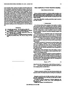
Fig. 1. Sampling data non-uniformly with a ZOH reconstruction pre-processing, thereby reducing the complexity of the system. This allows high-frequency analogue signals to be sampled at much lower sample rates and yet avoid the addition of any aliases in their digital spectra. Figure 1 illustrates the concept of applying random sampling and reconstructing them back by using a zero-orderhold (ZOH) reconstruction device (note that since the sample time is non-uniform, the ZOH-reconstruction will not be a time invariant system). More recently, other texts have commented on non-uniform sampling theory and its applications (See e.g. Marvasti [2001], Bilinskis [2007]), demonstrating its advantages and benefits. The non-uniform sampling strategy has been used for the implementation of broad-band measurement instruments (Filicori et al. [1989]). Furthermore, investigators have
In classical digital controller design, the sampled signals are always considered to be periodic and equally timespaced. But variations in the sample times are inevitable during operation and much efforts have been researched to reduce these effects (Albertos and Crespo [1999]). The motivation for this research is to investigate practical ways of creatively using these variations in the sample period or even utilizing a deliberate non-uniform sampling scheme to extract some benefits from it, principally as a result of enabling a lower sampling frequency without compromising the operating bandwidth of the digital compensator, with a reduction in the overall processing. This paper is structured as follows. Section 2 presents the theoretical background of alias-free sampling describing its potential benefits, followed by a brief description of an IIR filter. Section 3 highlights the design of a non-uniform sample time controller and the consequence of using the z-operator to implement it. Sections 4 proposes a solution to the issues rising from using the z-operator by using the modified delta operator. Section 5 describes the future work and finally the conclusion.
16 14 12
Amplitude
10 8 6 4 2 0
2.1 Alias-free sampling Alias-free sampling is purely an exercise of identifying the true spectral content of a signal. A sampling scheme that demonstrates such superior abilities for alias suppression is the additive-random sampling scheme (Shapiro and Silverman [1960]), which is primarily based on the assumption that the successive sampling intervals {ti , ti+1 } are statistically independent and identically distributed. These sample intervals were characterized by their mean value µ and a standard deviation σ. The sampling mode is given as: ti = ti−1 + Ti , i = 0, 1, 2, . . . (1) where ti−1 is the i − 1th sampling time and Ti is a realization of a random variable which can be generated by a pseudorandom number generator algorithm i.e. linear feedback shift registers. When a non-uniform sample time is used, the variances of the sample point locations sum up, so that after some time the probability of the sampling points along the time axis becomes constant. Therefore the non-uniformity between sample points should be implemented accurately
50
100 Frequency [Hz]
150
200
18 16 14 12 10 8 6 4 2 0
2. THEORETICAL BACKGROUND
0
Fig. 2. Uniformly sampled data. Sampling below the Nyquist rate causes aliases which can clearly be seen to have corrupted the signal
Amplitude
demonstrated the ability of random sampling to recover a DC signal immersed in noise (Carrica et al. [2001]). Nonuniform sampling has also recently been applied to FIR filtering (Tarczynski et al. [1997]). However, despite being a popular area for research in digital signal processing, it has received scant attention in the field of digital control. This could be due to the fact that unintended variations or any sort of non-uniformity in the sampling instants have always been seen as a threat in feedback control systems as they could cause degradation in the control performance and may even lead to instability (Marti et al. [2001]). Either way, as far as the authors can tell, there has been no research reported investigating the opportunities of using a non-uniform sampling rate for feedback control systems.
0
50
100 Frequency [Hz]
150
200
Fig. 3. Non-uniformly sampled data. Adding variation to the sampling scheme can mitigate the effects of aliases so that some probabilistic requirements are met, or else the required alias suppression effects will not be achieved. The randomness introduced in the sampling time can be controlled by one parameter, the ratio of σ and µ (which is the standard deviation and mean sample rate). Note that a ratio σ/µ of zero will signify uniform sampling. The ability to distinguish frequencies depends on the ratio σ/µ used when generating the sampling point process. Obviously, the more the ratio σ/µ, the more alias suppression can be achieved, but too much variation can introduce unacceptable statistical errors in the whole process. Therefore an intermediate value must be used that will accomplish the intended effect. In Figure 2, an 80Hz sine wave is sampled at 100Hz with a uniform sampling scheme. Obviously, due to the slow and constant sample rate, duplicate frequencies appear in the spectrum of the ‘under-sampled’ signal. Figure 3 shows the result achieved when the non-uniform additive pseudo-random sampling pattern is used to acquire the sample instances. The pattern has an average non-uniform
Fig. 4. Applying a deliberate non-uniform sampling rate in a closed-loop sample rate of 100Hz, with a variation ratio σ/µ = 0.2. The signal being sampled is a 80Hz sine wave. It can be seen that by using a non-uniform sample rate, aliases are converted into broadband noise which does not have the same implications as aliases (noise is incoherent) and hence is much less objectionable. It should be pointed out that when a set of data is sampled with a non-uniform sample rate, the usual FFT algorithms cannot be used. The results in Figure 3 are estimated by Equation (A.3) which is derived in the Appendix A. Alias-free sampling is theoretically possible whenever the random sampling sequences are stationary (Bilinskis and Mikelsons [1992]). In practical conditions of processing a finite number of samples, alias components are never eliminated completely but can only be suppressed by a finite amount. The mean sampling rate of a typical aliasfree sampling process is lower than the sampling frequency of the periodic sampling process that would be sampling the same signal. In other words, a non-uniform sampling scheme can allow the use of fewer numbers of samples and yet give accurate results. 2.2 The Infinite Impulse Response (IIR) Filter Controllers used in real-time control system implementations are primarily based on digital IIR filters that make use of the shift operator z −1 . The principal advantages of using recursive filters rather than nonrecursive Finite Impulse Response (FIR) filters are reduction of computation delays and improved computational efficiency as they use less memory resources, although it should be noted that the recursion introduces significant numerical issues that do not exist with FIR approaches. Typically, a general IIR type equation in the s-domain is defined as:
H(s) =
N (s) n0 + n1 s + · · · + nM sM = , D(s) 1 + m1 s + · · · + mN sN
(2)
It can be implemented digitally by making use of the shift operator and the coefficients can be approximated from the continuous plane to the digital domain through mapping techniques, e.g. bilinear transform. The resulting transfer function takes the form:
H(s) =
N (z) a0 + a1 z −1 + · · · + aM z −1 = , D(z) 1 + b1 z −1 + · · · + bN z −1
(3)
Fig. 5. The direct implementation structure
Fig. 6. The canonical implementation structure It is this filter (3) that needs to be implemented with a time varying sampling frequency.
3. SETTING UP THE NON-UNIFORM SAMPLE TIME CONTROLLER A closed-loop layout for enabling a non-uniform sample rate to an existing controller is shown in Figure 4. It comprises of the digital compensator, that will implement the control algorithm and a non-uniform sample times block which regulates the sampling process and provides the digital compensator with the current sample rate value to update its coefficients. In addition, there will be various delays associated with the controller implementation which includes the effects of the Zero-Order-Hold (ZOH) reconstruction and latencies during computation. The design layout is simplified, since the delays are ignored at all the frequencies in the bandpass. Although, during implementation this can be done only if the uniform sample rate is much higher than the bandpass frequency, ωs . A good selection of the sample rate fs , where fs = 1/T and 2Π = ωs , well above the control bandwidth can provide control engineers with certain freedom to design compensators in the continuous s-domain to the approximate zdomain to match their requirements. Therefore, the role of sampling in control systems is two-fold, it has to limit: • aliasing of frequencies within the control loop bandwidth • loss of phase and gain margin due to delays (primarily due to the ZOH) In order to implement the discrete controller using the z-operator, an implementation structure will have to be determined. These structures reflect the ways in which the discrete transfer functions can be interpreted both theoretically and diagrammatically. The most commonly used methods are the direct and canonical forms shown in
Figures 5 and 6, respectively. It is widely recognized that the canonical form has certain benefits over the direct form since there are fewer stored variables and shift operations and hence is the most popular choice for implementation.
n0 (ti − ti−1 ) + 2n1 (ti − ti−1 ) + 2m1 n0 (ti − ti−1 ) − 2n1 a1 = (ti − ti−1 ) + 2m1 (ti − ti−1 ) − 2m1 b1 = (ti − ti−1 ) + 2m1
2
1.5
1
0.5
0
a0 =
5
10
15
Fig. 7. Showing an undesirable transient. The filter coefficients are changed just once at t = 8s (4)
A point to be noted is that, if implemented in the correct way, this transient phenomenon will not occur in the case of non-recursive filters (Valimaki and Tarczynski [1996]). Furthermore, a recursive time varying filter is ‘transient-free’ only when its feedback coefficients are kept unchanged throughout the whole process. However, in this case, all the compensator coefficients will being changed and hence the transients will cause an undesirable behavior of the closed loop system. To better understand the concept of transients, consider the following experiment which is an emulation of a practical PID compensator based on IIR filtering, where the filter coefficients are changed just once at runtime at t = 8s. The compensator has the transfer function: 1 + 0.05s 1 + 0.2s . 1 + 0.01s 0.2s
And the fixed and continuous plant model is: 0.65 1 + 0.45s
The digital filter coefficients are updated by changing the sample time parameter ts. For simplicity, in this
Plant response Control signal
3
2.5
2 Output
The coefficients of any digital filter are dependent on the sampling interval, which are usually calculated just once at the start of the implementation. When a non-uniform sampling scheme is employed, the filter coefficients will have to be updated at each sample instant by using (4), which will allow the filter to retain its desired characteristics. However, in the case of recursive filters, the output signal may suffer from a transient phenomenon as the filter is loaded with its internal variables based on the previous coefficient set. The severity of transient signals depend on the filter input signal and the size of magnitude change in the filter coefficients.
P (s) =
0
time (s)
3.1 Repercussions of sample-time non-uniformity
H(s) =
Plant response Control signal
2.5
Output
In order to adapt to the varying sampling rate, simple formulas can be driven from (2) through discretization techniques, to be used by the control algorithm in every iteration. This will enable the coefficients of the compensator to be updated directly during the operation in order to preserve the desired filter characteristics. Consider the non-uniform sampling sequence {. . . , ti−1 , ti , . . . }, then the coefficients for a time varying 1st order compensator can then be given as:
3
1.5
1
0.5
0 0
5
10
15
time (s)
Fig. 8. Uncontrollable transients when using a nonuniform sampling pattern. The filter coefficients are changing at every sample instant demonstration only two filter coefficient sets are being used, set-1 from 0s → 8s (where ts = 0.02s), and set-2 from 8s → 15s (where ts = 0.01s). Figure 7 shows the control signal generated by the controller and plant response due to it. It is evident that the change in coefficients in the discrete compensator (at t = 8s) has significantly affected the control signal at the point of coefficient change. A solution to this problem was presented based on the assumption that images of recursive filters are running for each coefficient set that is ever encountered in the system, but only one of them is connected to the output at one time (Zetterberg and Zang [1988]). However, this approach requires a very large number of filters running in parallel which makes it increasingly complex. In practice, this is not computationally viable and further modifications to this method were suggested (Valimaki et al. [1995]) for transient suppression that could give an acceptable performance at a reasonable implementation complexity. The problem that has to be addressed in the case of nonuniform sample
Plant response Control signal 2.5
Output
2
Fig. 9. The Modified delta canonical structure
1
time IIR filtering is slightly more complicated, especially when the sample time parameter ts is changing at every instant, introducing uncontrollable transients. Figure 8 demonstrates the effect of transients occurring due to a continuously varying sampling time pattern. The pattern has an average sample rate of 50Hz (ts = 0.02s), with the variation ratio σ/µ = 0.2. Clearly, the control signal is suffering from transients that could destabilize the system. 3.2 The importance of implementation structure Recent investigators have highlighted the significance of choosing the right implementation structure for the purpose of transient reduction (Kovacshazy et al. [2001]). Using the proper structure for the controller realization can aid in suppressing transients, and the delta structure has been identified to assure smaller transients than other structures for small disturbances.
The delta operator provides a much superior performance over the fixed-point shift law implementation (Middleton and Goodwin [1990]) and can lead to much reliable and robust numerical control algorithms. Since the internal variables in the delta structure are no longer successive values of the same quantity, the operation is rather an accumulation of the previous values with the new values. A delta equivalent transfer function can be derived from the z based discrete function by using the following mapping: z −1 1 − z −1
4. IMPLEMENTING THE DELTA OPERATOR The discrete transfer function in the delta form can be written in identical form to that for the z operator (3), although the coefficient values will be different: H(δ) =
0.5
0
0
5
10
15
time (s)
Fig. 10. Output response using the delta operator. Demonstrating transient dependence on the filter structure forward path of the filter (Forsythe and Goodall [1991]). This modification has the important advantage that the internal variables have their maximum values which are of the same order as that of the input variable. The discrete transfer function is now written as: H(δ) =
p + d1 qδ −1 + · · · + d1 . . . dN rδ −n , 1 + d1 δ −1 + · · · + d1 . . . dN δ −n
(6)
where r is the last feed-forward coefficient.
3.3 The Delta transform
δ −1 =
1.5
c0 + c1 δ −1 + · · · + cM δ −n , 1 + r1 δ −1 + · · · + rN δ −n
(5)
The only adjustment needed in the implementation equations is that the original shift equations have to be replaced by additions.
Again, the coefficients need to be recalculated each time the sample time changes during the operation. The equations required for calculating the coefficients for a time varying 1st order delta compensator can be given as: n0 (ti − ti−1 ) + 2n1 (ti − ti−1 ) + 2m1 q = n0 2(ti − ti−1 ) d1 = (ti − ti−1 ) + 2m1 p=
(7)
It is worth mentioning that as the order of the filter increases, the coefficient calculations will have to take the prior sample rates into consideration. For example, assuming the non-uniform sampling sequence {. . . , ti−2 , ti−1 , ti , . . . }, then a 2nd order filter will need to take the values of ti−2 , ti−1 and ti into account to calculate the correct results. Figure 10 demonstrates the simulation carried on the same PID compensator used earlier, but with a modified delta structure implementation instead. It is evident that using the delta operator in the non-uniform sample time controller implementation can provide a better performance than its z counterpart in canonical realizations. 5. FUTURE WORKS AND CONCLUSION
4.1 The modified delta transform A modification of the filter structure can be seen in Figure 9, in which the feedback coefficients are moved into the
The paper described the concept of alias-free sampling highlighting its potential to suppress aliasing while processing signals at rates below the Nyquist limit. The paper
investigates the use of this approach for digital control applications. However, a major issue was identified when variations in sampling instants result in uncontrollable transients that can cause serious performance degradation. A simple control example was presented to demonstrate this effect and a solution to reduce it was also presented. The delta transform was found to provide a more robust implementation with the non-uniform sample rate. The next steps involve demonstrating the applicability with other controller structures and application to some real experimental hardware. Central questions related to the research that are yet to be answered are: • Can a non-uniform sampling pattern help improve the operating bandwidth of a control system? • What are its implications on stability?
A. Tarczynski, V. Valimaki, and G. D. Cain. Fir filtering of nonuniformly sampled signals. Acoustics, Speech, and Signal Processing, 1997. ICASSP-97., 1997 IEEE International Conference on, 3:2237–2240, 1997. V. Valimaki and A. Tarczynski. Modifying fir and iir filters for processing signals with lost samples. Proc. NORSIG 1996, 1:359–362, 1996. V. Valimaki, T. I. Laakso, and J. Mackenzie. Elimination of transients in time-varying allpass fractional delay filters with application to digital waveguide modeling. Proc. Int. Computer Music Conference, pages 303–306, 1995. L. H. Zetterberg and Q. Zang. Elimination of transients in adaptive filters with application to speech coding. Signal Processing, 15(4):419–428, 1988. Appendix A. NON-UNIFORM TIME DISCRETE FOURIER TRANSFORM
REFERENCES P. Albertos and A. Crespo. Real-time control of nonuniformly sampled systems. Control Engineering Practice,, 7(4):445–458, 4 1999. I. Bilinskis. Digital Alias-free Signal Processing. John Wiley & Sons Ltd, 2007. I. Bilinskis and A. Mikelsons. Randomized Signal Processing. Prentice Hall, London, 1992. D. Carrica, M. Benedetti, and R. Petrocelli. Random sampling applied to the measurement of a dc signal immersed in noise. IEEE Transactions on Instrumentation and Measurement, 50(5):1319–1323, 2001. F. Filicori, G. Iuculano, A. Menchetti, and D. Mirri. Random asynchronous sampling strategy for measurement instruments based on nonlinear signal conversion. IEE Proceedings Science, Measurement and Technology, 136 (3):141–150, 1989. W. Forsythe and R. M. Goodall. Digital Control: Fundermentals, Theory and Practice. 1991. R. M. Goodall, S. Jones, and R. Cumplido-Parra. Digital filtering for high performance real-time control. IEE Colloquium on Digital Filters: An Enabling Technology (Ref. No. 1998/252), pages 7/1–7/5, 1998. T. Kovacshazy, G. Peceli, and G. Simon. Transient reduction in reconfigurable control systems utilizing structure dependence. IEEE Instrumentation and Measurement, 2001. N. R. Lomb. Least-squares frequency analysis of unequally spaced data. Astrophysics and Space Science, pages 447– 462, 1976. P. Marti, J. M. Fuertes, G. Fohler, and K. Ramamritham. Jitter compensation for real-time control systems. RealTime Systems Symposium, IEEE Proceedings, pages 39– 48, 2001. F. Marvasti. Non-uniform Sampling: Theory and Practice. 2001. R. Middleton and G. Goodwin. Digital Control and Estimation: A Unified Approach. Prentice Hall Professional Technical Reference, 1990. ISBN 0132116650. R. W. Ramirez. The FFt Fundamentals and Concepts. Prentice Hall PTR, 1984. H. S. Shapiro and R. A. Silverman. Alias-free sampling of random noise. SIAM Journal on Applied Mathematics, 8(2):245–248, 1960.
Many techniques exist in literature for estimating the spectral content of unevenly sampled data (see e.g. Lomb [1976], Marvasti [2001]). Although, a simple method based on numerical integration is described here. Consider the expression of the standard discrete Fourier transform (DFT) as given by Ramirez [1984]:
Xd (k∆t) = ∆t
N −1 X
x(n∆t)e−j2Πk∆f n∆t
(A.1)
n=0
where the variables have the following definitions: Xd (k∆t) x(n∆t) N ∆t ∆f n k
set of Fourier coefficients discrete set of samples number of samples considered time between samples sample interval in the frequency domain time sample index frequency component index
assuming that the sampling scheme is defined according to Equation (1), then the spectrum can be estimated as:
Xd (k∆f ) = ∆t
N −1 X
x(ti )e−j2Πk∆f ti
(A.2)
n=0
where ti is the non-uniform sample time instant The approximation of the Fourier coefficients can further be improved by applying other sophisticated numerical integration rules (although the improvement in approximation will come at the cost of increased complexity of the expression). Consider the following substitution where y(ti ) = x(ti )e−j2Πk∆f ti the result with trapezoidal integration can be expressed:
Xd (k∆f ) = ∆t
N −1 X n=0
[y(ti ) + y(ti+1 )]
(ti+1 − ti ) 2
(A.3)