Implementation of TPSA in the Mathematica Code LieMath - CERN

Proceedings of EPAC 2006, Edinburgh, Scotland

WEPCH067

IMPLEMENTATION OF TPSA IN THE MATHEMATICA CODE LieMath D. Kaltchev, TRIUMF, Vancouver B.C., Canada Abstract

Pyramids of Coefficients

The Lie Algebra package LieMath written in the Mathematica language constructs the beamline map in a singleexponent Lie generator form. The algorithm (a BCH-based map concatenation) has been recently enhanced with Truncated Power Series Algebra (TPSA) techniques. The polynomials produced by the series expansion of the Hamiltonian are replaced with arrays of coefficients (derivative structures) and the Poisson bracket and BCH are defined as operations on such structures. We have confirmed the statement that using automatic differentiation instead of symbolic operations increases the speed by least an order of magnitude. The code is equipped with a MAD parser and a normal form block allowing it to extract nonlinear chromaticity and amplitude detuning. The notebook was applied in FFAG studies and may be useful for the linear collider final focus or collimation systems.

The expansion of a real-valued function of n variables x = {x1 , x2 , . . . , xn }, truncated at order m, is:

INTRODUCTION In the BCH-based map concatenation, the computationally intensive part is calculation of the Poisson brackets (PB). Therefore, differential algebra libraries are needed to carry out fast computations with polynomials and vector functions of polynomials. The map may be created on a symbolic computational system such as Mathematica [1], [2], [3]. Usually, as it was the case with the LieMath code reported in [3], one relies on the symbolic engine to perform operations on multivariate polynomials, such as product, derivative, truncation etc. We have recently implemented in LieMath some Truncated Power Series Algebra (TPSA) techniques allowing us to speed up the above operations and also to produce parameter dependent Taylor maps – maps with knobs [7]. The main question addressed here is how to implement the pyramid structure of polynomial coefficients and efficiently handle the index set manipulation. We use direct addressing with a linear index array and preprocessing [5], [6]. In general, the implementation of TPSA improved the notebook runtime by around a factor of ten – see the last Section.

TPSA IN LIEMATH This section describes the algorithm allowing one to replace the polynomial operations in BCH with operations on coefficient arrays (derivative structures).

f (x) =



Fk xk11 . . . xknn =

|k | ≤ m



Fk xk

(1)

|k | ≤ m

|k| ≡ k1 + k2 + · · · + kn , where the multi-index k = {k 1 , k2 , . . . kn } is a vector of nonnegative integers indicating the term in the series and Fk is an array of series coefficients. F k is also the array of partial derivatives of f (with factors k l ! thrown in). It can be visualized is an n-dimensional pyramid where n specifies the dimension – linear, triangular, and pyramidal arrays, and m the size. Below we will call F k the derivative structure (DS), or simply the pyramid of f . One can join all index vectors k into one array (index set) Γm n . The index set can be built as follows: Γm n ≡ {k1 , k 2 , . . . , k L } =

Join C[p, n] (p = 0, 1, · · · )

(2)

wherethe total  number of entries L is the binomial coeffim + n cient and C[p,n]) are the Compositions of p of m order n, i.e. all different arrangements of n nonnegative integers whose sum is p. A function generating C is available in Mathematica.

Poisson bracket as a pyramid operation Let f, h, u, v be the polynomials produced by the truncated series expansions of the Hamiltonian and F, H, U, V the associated pyramids. The basic idea is: if h is given as an arithmetic operation combining u and v and the pyramids U and V are known, then one needs to define a corresponding pyramid operation on U and V that yields H. To encode the Poisson bracket only power and derivative are of interest since addition and multiplication by a number are performed coordinatewise, as in matrix addition and multiplication by a constant.

Indexing and Speed Although in Mathematica it is not a syntactic problem to index directly one array with another, even when their dimensions are arbitrary, we choose to work with a linear index, which means simply dumping all F k into a linear array F (l), l = 1, . . . L. The method of addressing and the order in which the entries F (l) are stored in the computer memory have been chosen in three alternative ways:

05 Beam Dynamics and Electromagnetic Fields D02 Non-linear Dynamics - Resonances, Tracking, Higher Order

2077

WEPCH067

Proceedings of EPAC 2006, Edinburgh, Scotland

A) the order of F (l) is as in (1), i.e. determined by the Compositions operator. A reference array lists all the indices needed for the DS Poisson bracket (PBDS). For each argument U, V subsets of Γ are created and stored together with information on what to do with the subset. A subset corresponds to a group of pyramid entries called a box. When the PBDS is actually called, only the box elements are operated upon. This method saves time at the expense of space and only requires one to encode a few manipulations on lists of integers. However, this is may not be the optimum solution for operations on sparse arrays, which occur since in some expressions only a few of the variables are present. B) F (l) is reordered in the same way as the differential algebra vector in [5], i.e. according to decimals in base m + 1. This brings the advantage that for the product the resultant coefficients can be automatically stored into the correct location, thus avoiding multiple operations on zeros. A reference array is still used. The derivative is computed as in A. C) F (l) is reordered according to the nested index SCALARNEST in [6]. With the method A, the time needed to concatenate two elements with a BCHDS that contains terms to O(6) (see below) is a constant: 0.22 sec on a 1 GHz processor for n=6 and map order M=3. With method B, as well as with the analytical BCH, this time varies depending on the optical element. In general, replacing A with B did not bring any substantial improvement in speed which can be explained with the built-in ability of Mathematica to operate on sparse structures. Work in this direction continues.

LIEMATH The map transforms a vector of canonical coordinates x = (x, px , y, py , cτ, pτ ). The dimension of phase space n may be larger than 6, if a nonlinear optimization is required (last Section). The input conforms closely to the standard format, which is made possible by a Mad parser written in the same language. MadX and Dimad beamline descriptions work, if a flow-control command liemath is added immediately after use. The algorithm is as outlined in [3], [8], [10]. However, the BCH formula is replaced by its pyramid equivalent BCHDS. At first, Γm n is created and the generators −Lp Hp (x) are series-expanded to order m = M + 1 and converted into pyramids F k . Above Lp and Hp are the length and the Hamiltonian of the p-th optical element. For a particle with energy E, assumed to be constant, the Hamiltonian is: 1/2  pτ eAs 2pτ 2 2 2 + pτ − px − py − − . H = −(1+hx) 1 − β0 β0 p 0 (3) The momenta have been scaled by the design momentum p0 . Also pτ = −(E − E0 )/p0 c and cτ = c(t − t0 ) is the

2078

time of flight relative to the reference particle. In the field  . s (1 + hx), where A  is the vector expansion term A s = A potential and s the unit vector in direction tangent to the reference trajectory. We use eA s /p0 up to and including octupole terms, see e.g. [9]. The kick factorization of an element is made by replacing it with a Lie operator and a following linear matrix. All matrices are moved to the end of the lattice, which changes each Lie operator with a similarity transform. For purely numerical maps, using the DS operators in the last step does not give much advantage because of the sparsity of the polynomials involved. Next, all nonlinear generators are combined into one with BCHDS: BCHDS(F, G) = F + G + +

1 1 :F : G + : F :2 G+ 2 12

1 1 : G :2 F + · · · + : G :2 : F :2 G + O((F, G)6 ); 12 120 : A : B ≡ PBDS[A, B]), (4)

where F and G are the pyramids of two polynomials whose linear terms are removed and O((f, g) 6 ) means terms of order ≥ 6. Applying on this generator the formal expansion of the Lie exponent (in DS form) yields the Taylor map. For periodic lattices, this one-turn map is converted to its normal form by using symbolic transformations as in [4].

RESULTS Computing time For purely numerical maps, the notebook runtime is around one minute per 100 elements. This time is reduced ∼ 3 times for a BCH of order O((f, g) 4 ). Using BCHDS in the concatenation loop (4), instead of the symbolic BCH, improves speed since in intermediate calculations the symbolic system attempts to store all terms, so truncation of the orders ≥ m becomes absolutely necessary, while with TPSA the polynomials are in a sense always automatically truncated in the desired order. To confirm the above statement we have compared the time of BCHDS and the untruncated BCH. Only some fraction, picked up randomly, of the f and g pyramids is populated with nonzero real numbers. The improvement in speed due to TPSA reaches a factor of 10 3 for large-size (n > 4, m > 3) and dense (most entries nonzero) pyramids. The maximum improvement is observed when all coefficients are symbols. In another test (Table 1) we have timed the BCH loop for a beamline of 70 elements. The result from the symbolic BCH is truncated at order m after each element. Table 1: BCH loop time in sec (lattice as in [1]) M 3 4

BCHDS 15 52

symbolic BCH 125 846

05 Beam Dynamics and Electromagnetic Fields D02 Non-linear Dynamics - Resonances, Tracking, Higher Order

Proceedings of EPAC 2006, Edinburgh, Scotland

WEPCH067

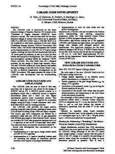
Figure 1: LieMath output showing the (linear) dependence of the elements T126, T346, U1266 and U3466 on the strengths of the two sextupole families S1 and S2. See the discussion in [1] and [11].

Figure 2: Strong interleaved sextupoles – lattice as in [1]. The particle is a 50 GeV electron with x0 = 3 σ (σ = 1.5 10−6 m). The Dimad result (sineand cosine-like trajectories) is also shown.

Numerical nonlinear optimization One natural extension of the algorithm allows us to get numerical maps depending on nonlinear parameters (maps with knobs [7]). Consider a beamline for which Q parameters nl1 , nl2 , . . . , nlQ have been declared to be variables. To create dependence on these parameters, the above names are appended to the coordinate vector: x = {x, px , y, py , cτ, pτ , nl1 , nl2 , . . . nlQ } and the value of m is increased. No other changes in the algorithm are needed. For instance, increasing the map order from two to three produces linear dependence on sextupole strengths, making it possible to match chromaticities and second order map elements. An example based on the lattice in [1] is shown on Figure 1.

Agreement with numerical integration of EOM Fig. 2 and 3 present results of single-pass tracking through the Mathematica Taylor map of order M for two lattices: one with strong interleaved sextupoles (SLC final focus [1]), and another – an FFAG cell with a very large momentum offset required [3]. For each optical element, we have solved numerically the equations of motion derived from (3) with unexpanded square root. For test purpose, no approximations are made in the Hamiltonian. The plots show, for a particle that starts with x = {x0 , 0, 0, 0, 0, pτ,0}, i.e. δ = (1 − 2pτ,0/β0 + p2τ,0 )1/2 − 1, the relative deviation of final x LIE from the numerical result xNUM , assumed to be exact.

Figure 3: A large momentum offset and lattice as in [3]. The particle is a muon (γ = 190) and x 0 = 1 cm. The result from 7th-order tracking with Cosy is also shown.

In both cases the agreement is limited for large M , which is explained with the omitted higher orders in the BCH expansion (4).

REFERENCES [1] N. J. Walker, J. Irwin, M. Woodley, “Analysis of Higher Order Optical Aberrations in the SLC Final Focus”, using Lie Algebra Techniques, Proc. of PAC 1993. The lattice we have used can be found as Demo 7 in Dimad: ftp://csftp.triumf.ca/pub/CompServ/dimad [2] J. Irwin, Analytic Nonlinear Methods for Beam Optics, in Proc. PAC 1997. [3] D. Kaltchev, Building Truncated Taylor Maps with Mathematica and Applications to FFAG, in Proc. EPAC 2004. [4] Chunxi Wang and Alex Chao, “Analytic Second- and ThirdOrder Achromat Designs”, Proc. of PAC 1995. [5] Berz M., “ Differential algebraic description of beam dynamics to very high orders”, Particle Accelerators 24, 109 (1989), pp 109-124. [6] R. Neidinger, “Computing Multivariable Taylor Series to Arbitrary Order”, Proc. of Intern. Conf. on Applied programming languages, San Antonio (1995) pp. 134-144 [7] M. Berz and K. Makino, COSY Infinity Version 8.1. [8] Tanaji Sen, Y.T. Yan, J. Irwin, Liemap : A Program for Extracting a One-turn Single Exponent Lie Generator map [9] Johan Bengtsson, Doctorate Thesis CERN 88-05. [10]A. Dragt and E. Forest, J. Math. Phys. 24 (12), 1983. [11]J. Murray, K. Brown, T. Fieguth , SLAC-PUB-4219 (1987).

05 Beam Dynamics and Electromagnetic Fields D02 Non-linear Dynamics - Resonances, Tracking, Higher Order

2079