sensing and image processing applications can be implemented efficiently on ...
The properties of algorithms and application that make for efficient GPU.
IMPLEMENTING ALGORITHMS FOR SIGNAL AND IMAGE RECONSTRUCTION ON GRAPHICAL PROCESSING UNITS SANGKYUN LEE
AND STEPHEN J. WRIGHT∗
Abstract. Several highly effective algorithms that have been proposed recently for compressed sensing and image processing applications can be implemented efficiently on commodity graphical processing units (GPUs). The properties of algorithms and application that make for efficient GPU implementation are discussed, and computational results for several algorithms are presented that show large speedups over CPU implementations. Key words. Graphical processing units, compressed sensing, image denoising, image deblurring. AMS subject classifications. 65Y10, 90C47, 90C20, 90C06
1. Introduction. Parallel computation has long been recognized as a means of speeding up computationally intensive numerical computing tasks. A great variety of architectures has been developed over the years to support different types of parallel computation. With the current ubiquity of multicore architectures, parallel processing has become the dominant paradigm in computing. Most personal computers also contain another type of parallel processing device: graphical processing units (GPUs). GPUs were developed for real-time rendering or 3D graphics, but are increasingly being adopted for massively parallel numerical computating. GPUs feature a many-processor architecture and high-bandwidth memory that maximize multithreading performance, along with faster arithmetic units than those on CPUs. Many recent studies have reported significant performance boosts by using GPUs to run critical numerical computing tasks in various applications, including pattern analysis [7, 15], biomedical imaging [17], DNA sequence alignment [28], molecular modeling and simulation [29, 32], multibody dynamics [30], and quantum chemistry [31]. Our focus in this paper is on GPU implementations of algorithms that have been proposed recently for reconstruction of sparse signals from random observations (compressed sensing) and for image denoising and deblurring. These problems typically involve a large number of unknowns but, unlike many problems in numerical computing, the amount of data needed to specify the problem typically is often less than the number of unknowns. The major computational operations that are used in the algorithms we described here — which are among the most effective algorithms available for these problems, even when implemented on CPUs — are readily implemented with high efficiency on GPUs. In this paper we introduce NVIDIA’s GPUs and describe the CUDA software platform that can be used to implement algorithms on these GPUs. We then describe the applications and algorithms, discuss some details of the GPU implementations, and give computational results that compare the speed of implementations on the CPU host with the speed of the GPU implementation. Since the cost of GPUs is so low (hundreds of dollars) and the speedups so high (two orders of magnitude and more), GPU implementations provide a remarkable extension of numerical computing capabilities in certain areas at an extremely low cost. 2. Hardware and Software Platform. ∗ Computer Sciences Department, University of Wisconsin, 1210 W. Dayton Street, Madison, WI 53706, USA; {sklee}{swright}@cs.wisc.edu
1
2
S. LEE AND S. J. WRIGHT
GPU 8 Scalar Processors SP
SP
SP
SP
SP
SP
SP
SP
T1
T2
T3
T4
T5
T6
Block 1,2
Block 1,3
Block 2,1
Block 2,2
Block 2,3
Block 3,1
Block 3,2
Block 3,3
Shared memory Texture memory Constant memory
Streaming Multiprocessor Multiprocessor
Global memory A task
Fig. 2.1. A schematic view of a GPU.
Fig. 2.2. A thread execution configuration.
2.1. NVIDIA GPUs. NVIDIA provides a wide range of GPU products that can be used for general computing as well as for their original purpose of real-time rendering or 3D graphics. Here we briefly describe two recent models, the GeForce 9800 GX2 and Tesla D870. Both devices provide two GPUs whose processor and memory specifications are summarized in Table 2.1. In both products, each GPU has 128 processors called scalar processors (SPs), which run threads and access the shared or global memory concurrently. A streaming multiprocessor (SM) is composed of 8 SPs together with an instruction unit, 8192 registers, shared memory, and caches. Each GPU has a high-bandwidth global memory, which can be accessed from all 128 SPs in the same GPU. A schematic view of a GPU composed of these elements is shown in Figure 2.1. In these products, the memory bandwidth of the global memory in GPUs is much higher than the bandwidth of the host memory: GPU memory transfer rate is more than 60GB/s, whereas the host memory transfer rate is 6.4GB/s for DDR2-800 memory (the memory on our host PC), or 12.8GB/s for DDR3-1600 memory (the fastest presently available.) The GPUs are connected to a host computer via the PCI Express bus, which provides the maximum bandwidth of 8GB/s (PCI Express v2.0 ×16) between the host and GPU. Although this rate is much slower than the GPU-to-GPU transfer rate, it is actually faster than the host-to-host memory transfer rate for the DDR2-800 host memory that we use. Our host computer is a Dell Precision T5400 workstation, equipped with a 2.66GHz Intel quad-core processor and 4GB of main memory. Since our focus in this paper is on fine-grained parallelization of the algorithms in question, we use only a single GPU of the GeForce 9800 GX2 device. Multiple GPUs can be utilized if we overlay a coarse-grained parallelization on the algorithms described below. This could be accomplished by writing CPU-based parallel codes using pthread, MPI, or other parallel tools, but since such techniques are well understood, we do not investigate them in this paper. 2.2. Software Platform. The Compute Unified Device Architecture (CUDA) is NVIDIA’s software platform for GPUs [24]. It is an extension to the the C++ language that allows users to write thread execution configurations, manage device memory, and do thread synchronization. CUDA splits a task into a grid of blocks, where a block is composed of a set of threads. (An example of a grid composed of nine blocks, each
SIGNAL AND IMAGE RECONSTRUCTION ALGORITHMS ON GPUS
Device name # GPUs # Streaming Multiprocessors Number of Scalar Processors Memory size GPU memory bandwidth Host communication bandwidth
GeForce 9800 GX2 2 16 per GPU 8 × 16 per GPU 512MB per GPU 64GB/s per GPU 8GB/s
3
Tesla D870 2 16 per GPU 8 × 16 per GPU 1.5GB per GPU 76.8GB/s per GPU 4GB/s
Table 2.1 The specifications of NVIDIA GPUs.
with six threads, is shown in Figure 2.2.) These blocks are scheduled to run on the multiprocessors of the GPU. CUDA uses a single-instruction multiple-thread (SIMT) model, which means that the threads running in a multiprocessor share the same code but run at possibly different states with different streams of data. CUDA also provides GPU-accelerated libraries for basic linear algebra operations (CUBLAS [22]) and discrete Fourier transforms (CUFFT [23]). In CUDA, each GPU thread receives its own set of dedicated registers, unlike threads that run on CPUs, which typically share registers. This design helps minimize the costs of context switching on GPUs. When registers are shared, their contents must be stored in memory when one thread leaves a processor, and new values for the entering thread must be loaded from memory. Because memory transfers are about one hundred times slower than computations, avoidance of register content copies adds greatly to the benefits of fine-grained parallelism in CUDA. On the other hand, although multiprocessors contain a huge number of registers, the dedication of registers to threads limits the number of threads that can be simultaneously scheduled on a multiprocessor. The applications most suited to GPU implementations are those that are intensive in computation, for which the ratio of computation to memory accesses is high. Because CUDA provides faster memory accesses to coalesced patterns and spatially local patterns, operations on dense matrices and two-dimensional image data can be implemented efficiently. Since the shared memory in streaming multiprocessors can be accessed as fast as the registers (provided there is no bank conflict), operations that apply the same small data elements to different locations of a large data set can also be optimized. However, global memory size and host communication speed are limiting factors in any implementation, and both should be controlled carefully. Tasks should be large enough to keep all multiprocessors busy so that the latency of memory operations does not affect the overall efficiency too greatly. We refer to Appendix A for further details on maximizing the efficiency of CUDA programs on GPUs. 3. Compressed Sensing. 3.1. Problem Description. In compressed sensing, we seek to identify a signal that is known to be sparse, that is, when represented as a set of n coefficients in some basis representation, only S � n of the coefficients are nonzero. We aim to recover the signal from a set of m observations, with m < n, where each observation is some linear function of the signal — a linear combination of the coefficients in the basis representation. The observation vector y ∈ IRm can thus be expressed in terms of the signal coefficient vector x by y = Ax, where the m × n matrix A is referred to as the
4
S. LEE AND S. J. WRIGHT
sensing matrix. Under certain assumptions on A, we can recover the true x by solving the problem min kxk1 subject to Ax = y,
(3.1)
which is the solution of the underdetermined linear system Ax = y with smallest `1 -norm. The crucial assumption on A, referred to as the restricted isometry property (RIP), essentially requires that each column submatrix of A for which the number of columns is comparable to S is almost orthonormal. This property ensures that any two signals of sparsity at most S retain their distinctiveness when operated on by A, so that they give rise to significantly different observation vectors. When A has such a property, the formulation (3.1) yields the true signal even when m is only a modest multiple of the number S of nonzero coefficients in the signal. When the observation vector y contains error, such as measurement noise, it is inappropriate to enforce the constraint Ax = y exactly. Here, we replace (3.1) by the following weighted formulation: min φ(x) := x
1 kAx − yk22 + τ kxk1 , 2
(3.2)
for some regularization parameter τ > 0. Note that for τ ≥ τmax the solution is x = 0, where τmax := kAT yk∞ .
(3.3)
Theory concerning the effectiveness of these formulations for finding sparse solutions of Ax = y can be found in the papers of Donoho [12, 11], Cand`es and Tao [5], and Cand`es, Romberg, and Tao [4]. Donoho [10] and Cand`es [6] give introductions to compressed sensing and discuss the various contexts in which these problems arise. 3.2. Algorithms. The optimization formulations above are conceptually simple — (3.1) can be written as a linear program and (3.2) as a convex quadratic program, with a suitable splitting of the variable x — but their difficulty arises from their high dimensionality (m and n large) and the fact that A is dense in many applications of interest. Many algorithms have been proposed, the vast majority of which do not require the full matrix A (or significant submatrices of A) to be stored or factored explicitly. Rather, they require numerous matrix-vector products involving A and AT to be performed. Fortunately, there are interesting matrices A that satisfy RIP for which such products can be calculated economically. For example, if A consists of m rows randomly drawn from an n-dimensional discrete cosine transformation (DCT), the products Au and AT v can be computed in O(n log n) operations. The same complexity estimate is true if we work with signals in the complex domain (A, x, and y containing complex elements), where A consists of m rows randomly drawn from a discrete Fourier transform (DFT). As a sample of the vast algorithmic literature, we mention the iterative thresholding / shrinking (IST) approach [9, 13]; extensions of this approach [21, 2] based on the optimal first-order methodology of Nesterov [19, 20]; a variant of IST that uses a “continuation” strategy of successively reducing the parameter τ in (3.2) [16]; interiorpoint methods [27, 18, 3]; and gradient projection applied to the bound-constrained quadratic programming formulation of (3.2) [14]. We focus in this paper on the SpaRSA approach of [33], which can be viewed as an accelerated variant of IST. From the current iterate xk , SpaRSA obtains the new
SIGNAL AND IMAGE RECONSTRUCTION ALGORITHMS ON GPUS
5
iterate xk+1 by solving the following subproblem: 1 xk+1 = arg min αk kz − xk k22 + (z − xk )T AT (Axk − y) + τ kzk1 z 2 � � 2 τ 1 = arg min z − xk − (1/αk )AT (Axk − y) 2 + kzk1 , z 2 αk
(3.4a) (3.4b)
for some αk > 0. The subproblem (3.4a) is the same as (3.2) except that the true Hessian AT A replaced by αk I, and a constant term is omitted. It is separable in the components of z, so it requires O(n) operations to solve (a closed-form solution is easy to derive), in addition to one matrix-vector multiplication each by A and AT , which are required to form the term AT (Axk − y). Different variants of SpaRSA are distinguished by different strategies for choosing αk . A nonmonotone approach (that does not necessarily yield a decrease in the objective (3.2) at each iteration) uses a choice of αk inspired by Barzilai and Borwein [1]. Denoting by sk := xk − xk−1 the difference between the last two iterates and y k := AT Ask the difference between the gradient of the sum-of-squares term (1/2)kAx − bk22 at the last two iterates, this variant sets αk =
kAsk k22 (sk )T y k = . (sk )T sk ksk k22
(3.5)
(Note that αk lies in the spectrum of the Hessian AT A, so in this sense, αk I is a plausible approximation to AT A.) A monotone variant uses the value (3.5) as an initial guess, then repeatedly increases αk by a constant factor η > 1 until xk+1 obtained from (3.4) has a lower function value than xk . The performance of SpaRSA (and other IST methods) generally degrades as the regularization parameter τ is reduced and the solutions x become more dense. Much of the practical efficiency can be recovered, however, by the use of a continuation strategy. We start by using SpaRSA to solve (3.2) for a larger value of τ , then decrease τ in steps toward its target value, using the solution for the previous value of τ as the starting point for each successive τ value. In the results report below, we specify the number of continuation steps C and step from the starting value τ0 = 0.8τmax to the target value τC = τ in C steps τ1 , τ2 , . . . , τC , where log τl = log τ0 + (l/C)a (log τC − log τ0 ).
(3.6)
Here, a ≥ 1 is a parameter governing the “bunching” of τl values near the target τ . (The value a = 1 leads to constant ratios τl+1 /τl , while larger values of a causes these ratios to become larger as l increases.) Implementations of SpaRSA and other algorithms often include an optional postprocessing step known as debiasing, in which the regularization term is dropped from the objective in (3.2) and an unconstrained least squares problem is solved, with the zero components of x from the main SpaRSA algorithm discarded. The last step is often performed with a conjugate gradient approach, for which the major operations at each iteration are multiplications by A and AT and some Level 1 BLAS calculations, just as in the main SpaRSA algorithm. We would thus expect the debiasing step to be implemented as efficiently on a GPU as the main SpaRSA algorithm. For simplicity, however, we did not include the debiasing feature in the implementations described in this paper.
6
S. LEE AND S. J. WRIGHT
3.3. GPU Implementation. For efficient GPU implementation of SpaRSA, it is important that the sensing matrix A is one that can be stored compactly (and implicitly) and that matrix-vector products involving A and AT can be formed efficiently on the GPU architecture. The other major operations in SpaRSA — vector additions and inner products — are simple and can be implemented efficiently or using BLAS operations from the CUBLAS library [22]. We use CUBLAS library to compute `1 -norms and inner products, but for all the other operations we use our own routines for better performance. The total amount of storage used is a small multiple of n. Specifically, we need to store the current iterate xk , the candidate for next iterate xk+1 , the step sk , the gradient of the sum-of-squares term AT (Axk − y) (each of which requires n locations), and the vectors Ask and Axk − y (each of which requires m locations), together with whatever storage is needed to represent A. Compressed sensing experiments often make use of matrices A whose elements consist of numbers drawn independently from a random distribution about 0 with a common variance, or from a Bernoulli distribution (entries ±1 with equal probability). Such matrices are known to have good restricted isometry properties and thus allow effective recovery of sparse signals. However, they are not practical for GPU implementation, as they generally either require much more than O(n) storage, or are expensive to regenerate whenever needed. Matrices A consisting of randomly chosen rows from a discrete cosine transformation (DCT) (in the case of real data) or a discrete Fourier transform (for complex data) are much more suitable. Besides having satisfactory restricted isometry properties, such matrices can be stored compactly (just m locations are needed, to store the indices of the chosen rows), and implemented using the CUFFT library [23]. DCTs can be implemented using DFTs with O(n) pre- and post-processing steps, which can be executed efficiently on GPUs. In our GPU implementation, significant data transfer between the host machine and GPUs occurs only at the beginning and the end of the algorithm. The initial values of the variable x, together with the observation vector y, the m row indices defining A, the regularization parameter τ , and possibly some algorithmic parameters are copied to the GPU at the start, and the solution is returned at the end. The host CPU is still used for small computations, such as computation of the roster of τ values used in the continuation process, in scalar comparisons, and in checking of loop control variables. Further savings could be made in data transfers if the value x = 0 as the starting point in the continuation process (it usually suffices). We can also return a compressed version of the solution of (3.2), consisting of the nonzero components of x and their indices. Further, if numerous instances of (3.2) are to be solved in sequence for different data, data transfers for successive instances could be overlapped with computation. 3.4. Computational Results. We discuss results obtained with simple implementations of SpaRSA, applied to problems in which the signal is a sparse one- or two-dimension array, and the sensing matrix consists of randomly selected rows from a discrete cosine transformation (DCT). Noise may be added to the observation vector. Our main point of comparison is between • the runtime for the Matlab implementation running on the CPU of the host machine (which we refer to hereafter as the “CPU implementation”), and • the runtime for the CUDA-based GPU implementation. Both implementations use the same Matlab code to set up the problem and analyze the results, but the GPU code replaces the Matlab routine implementing SpaRSA with a functionally equivalent CUDA routine.
SIGNAL AND IMAGE RECONSTRUCTION ALGORITHMS ON GPUS
7
We note several distinctions between the two implementations. First, the GPU computations are carried out in single precision, while the CPU computations are in double precision. This is because the GPU cards we used support only singleprecision arithmetic. (Double-precision cards are only now coming on the market, and the CUDA environment and its libraries are being extended to run on them.) The lower accuracy of single precision computations creates significant issues for the GPU implementation of SpaRSA. The duality-based stopping criterion for each value of τ described in [33] cannot be implemented satisfactorily in CUDA. Inaccuracy in computation of the gap often makes it difficult to reduce the relative gap below about 10−4 , regardless of how many iterations are performed, for smaller values of τ ; no such difficulties are observed in the double-precision CPU implementation. In our implementation, we used a stopping criterion for each value of τ based on the relative change in objective value from one iteration to the next, namely, |φ(xk ) − φ(xk−1 )| ≤ 10−6 . φ(xk )
(3.7)
Still, as we see in the tables below, the GPU implementation sometimes requires slightly more iterations than the CPU implementation to find a solution of equivalent accuracy. A second difference between the implementations is the use of Matlab code for the CPU implementation vs. CUDA code (an extension of C++) for the GPU implementation. We believe however that a CPU implementation via C++ and mex files would show little if any improvement over the Matlab implementation. The major computational operations are DFT, DCT, and Level 1 BLAS operations, all of which are implemented with high efficiency in Matlab. In fact, we could speed up the GPU implementation further by using C++ calling code in place of the Matlab and mex software. Multiple data transfer requests on page-locked host memory could be made without having to wait for the completion of the previous requests, making room for other jobs in the host or GPUs. In our current Matlab / mex interface, data are stored in the Matlab memory, which is not page-locked, so overlapped data transfers require extra copies to page-locked host memory. Such transfers only degrade the performance, so we avoid them. We note several issues regarding initialization of GPU computations. The very first call to a CUDA utility function made by a process (for example, cudaGetDevice Count() which counts the number of CUDA-enabled GPUs, or cudaSetDevice() which selects a particular GPU) executes in about .01 seconds. The very first GPU memory allocation call issued by a process takes significantly longer than subsequence memory allocation calls: about .8 seconds. Following these initializations, GPUs still appear to need some “warming up” before they reach peak performance. For example, if we compute the `1 -norm of a vector of length 106 , the first call takes approximately 2.5 times as long as the second call. These overheads will be amortized over all the invocations of SpaRSA made by that process. In real situations, we can expect SpaRSA to be invoked multiple times to process different data sets (for example, different time slices of a signal) in sequence, or possibly to be used as one of a number of tasks running concurrently on the GPUs. Hence, we do not include these initialization overheads in our discussion of GPU execution times below. One-Dimensional Signal with DCT Sensing. Our first experiment is with a onedimensional signal with n components, in which the sensing matrix consists of m < n rows drawn randomly from an n×n DCT matrix. The signal consists of bm/5c spikes,
8
S. LEE AND S. J. WRIGHT
half of which have magnitude near 1 with the remaining half having magnitudes between 10−5 and 10−4 (logarithms uniformly distributed). There is also noise in the signal of order 10−6 on each element. Results are shown in Tables 3.1 and 3.2. In both tables, the SpaRSA algorithm was run with 10 steps of continuation, with three different target values of τ , shown in the first column of each table. The total iteration counts and for the GPU and CPUbased implementations are shown, as is the final mean-square error in the recovered solution. The quality of the solution is similar for both GPU and CPU implementations. For the GPU, we show total runtime after the selection of the GPU, the very first GPU memory allocation, and a few “warm-up” numerical computations unrelated to the algorithm. The reported time includes time for second and subsequent memory allocations and times for data transfers to and from the GPU. Two speedup figures are shown in the final columns of each table. The first is calculated by comparing total runtimes between the GPU and CPU implementations, and the second by comparing runtimes per iteration. Table 3.1 shows results for a sensing matrix of dimension 213 × 216 . For each value of τ , the GPU execution time was approximately 0.16 seconds, whereas the CPU implementations required about 5 seconds, resulting in speedups of 26 to 37 in total time. The average speedups per iteration are about 34, and are almost identical for all τ values, indicating that the speedup resulting from use of the GPU is quite stable and consistent. Note that each iteration of SpaRSA on the GPU (in which the main computational effort is two matrix-vector operations involving the sensing matrix) takes about 1.2 microseconds, versus about 40 microseconds for the CPU implementation. Table 3.2 shows results for a sensing matrix of dimension 217 × 220 , a factor of 16 larger in each dimension. Here the speedups are 51 to 61 (counting total runtime), and about 61 on average per iteration. The memory transfer between host and GPU takes more time, but this cost is amortized over a much longer execution time, so its effects on speedup figures is less deleterious. Moreover, the larger data set yields a larger number of thread blocks in our implementation, resulting in less idle time on the GPU’s multiprocessors. Each iteration of SpaRSA in the GPU implementation requires about 16 microseconds, compared to about one second in the CPU implementation. Two-Dimensional Signal with DCT Sensing. Our second result is for a sparse two-dimensional signal of length n, which can be thought of as an n ¯×n ¯ array of pixels where n = n ¯ 2 , only a small fraction of which are nonzero spikes. The sensing matrix consists of m rows randomly selected from an two-dimensional (¯ n×n ¯ ) DCT matrix. We choose the fraction of spikes to be .001, and set m to be 20 times the number of spikes. Each spike is chosen randomly to be +1 or −1, and the observations are corrupted by noise drawn independently from a Normal distribution, N (0, .0012 ). The values of regularization parameter τ on which we report are approximately the ones needed to produce results of good quality. For τ = .05τmax and τ = .1τmax where τmax is defined in (3.3), the algorithms recover approximately the same number of nonzero components as in the true solution. For τ = .02τmax we have a slightly under-regularized solution, with more spikes than the true solution. We report results in Table 3.3 for a problem with n = 216 and m = 1311, while Table 3.4 shows a larger problem with n = 220 and m = 20972. The relative performances of the two approaches are broadly similar to the one-dimensional case. For larger data sets, the advantage of the GPU implementation increases. Although the
SIGNAL AND IMAGE RECONSTRUCTION ALGORITHMS ON GPUS
τ /τmax .000100 .000033 .000010
iters 103 135 143
CPU time (s) 4.32 5.52 5.81
MSE 8.1e-10 1.3e-10 9.8e-11
iters 129 126 139
GPU time (s) 0.16 0.15 0.17
MSE 7.2e-10 2.0e-10 1.3e-10
9
Speedup total iter 26 33 37 34 35 34
Table 3.1 Computational results for a 1-D DCT sensing matrix of dimension 8192 × 65536, with 1638 spikes
τ /τmax 0.000100 0.000033 0.000010
iters 107 131 149
CPU time (s) 107.08 129.10 145.31
MSE 9.1e-10 1.7e-10 1.0e-10
iters 129 131 160
GPU time (s) 2.08 2.10 2.57
MSE 8.5e-10 1.6e-10 9.0e-11
Speedup total iter 51 62 61 61 57 61
Table 3.2 Computational results for a 1-D DCT sensing matrix of dimension 131072 × 1048576, with 26214 spikes
τ /τmax 0.10 0.05 0.02
iters 62 67 77
CPU time (s) 2.56 2.68 3.06
MSE 1.9e-05 4.8e-06 9.7e-07
iters 67 68 83
GPU time (s) 0.09 0.08 0.10
MSE 1.9e-05 4.8e-06 9.6e-07
Speedup total iter 27 30 32 32 30 32
Table 3.3 Computational results for a 2-D DCT sensing matrix of dimension 1311 × 65536, with 60 spikes
τ /τmax 0.10 0.05 0.02
iters 64 65 80
CPU time (s) 98.25 103.10 117.97
MSE 3.2e-05 7.9e-06 1.5e-06
iters 64 70 84
GPU time (s) 1.00 1.08 1.30
MSE 3.1e-05 7.9e-06 1.5e-06
Speedup total iter 98 98 95 102 91 95
Table 3.4 Computational results for a 2-D DCT sensing matrix of dimension 20972 × 1048576, with 1031 spikes
time to transfer data between host and GPU increases as the data set size increases, the speedups improve because of faster memory access on the GPU, the increase in the number of thread blocks (which improves GPU utilization), and the fact that the GPU can perform thread scheduling and switching efficiently, without intervention of operating systems. The limit of n. For the one-dimensional compressed sensing, the problem with sensing matrices of the dimension up to 219 × 222 can be solved on the GeForce 9800 GX2, whereas we can drive the dimensions up to 220 × 223 on the Tesla D870. Note that the size limit on GeForce 9800 GX2 is due to the limitation of the GPU memory, whereas the limit on Tesla D870 is due to the limitation imposed by the CUFFT library, which allows a maximum input length is 223 for 1-D transforms and 216 for each dimension for 2-D or 3-D transforms. Similar considerations yield a restriction on the size of two-dimensional compressed sensing problems that can be solved to n = n ¯ 2 = 222 . For problems with larger dimensions than these, we would need to implement more complicated decomposition and parallelization strategies that are
10
S. LEE AND S. J. WRIGHT
beyond the scope of this paper. 4. Image Restoration. Image restoration is an important task in image segmentation or computer vision applications. Regularization methodologies based on total variation (TV), introduced by Rudin, Osher, and Fatemi [26], are highly effective in removing noise, blur, or other unwanted fine-scale detail, while preserving edges. We report here on TV-regularized denoising and deblurring formulations, solved with a particularly effective primal-dual gradient descent approach described recently by Zhu and Chan [34]. The main computational operations in this algorithm include a difference operation (needed to calculate the TV-norm), DFTs and inverse DFTs (needed in the deblurring application), and various Level 1 BLAS operations and simple projection operations. All these operations require O(N ) operations, where N is the number of unknowns, with the exception of the DFT and inverse DFT procedures, which require O(N log N ) operations. All can be implemented efficiently on a GPU. After briefly discussing the formulation and the algorithms, we compare the efficiencies of CPU and GPU implementations. 4.1. Denoising. Given a domain Ω ⊂ IR2 (usually a rectangle) and an observed image f : Ω → IR, we recover a denoised image u : Ω → IR by solving the following problem in the appropriate function space: Z |∇u|2 +
min u
Ω
¯ λ ku − f k22 , 2
(4.1)
¯ is a regularization parameter. (Larger values of λ ¯ yield better fidelity to the where λ recorded image, while smaller values produce more cartoon-like images, with larger areas of constant intensity.) The notation | · |2 represents the Euclidean norm on IR2 , and the first term in the expression (4.1) is the TV seminorm of u. We can obtain saddle-point and dual formulations of (4.1) in function space by an appropriate redefinition of the TV seminorm. (Some details are given in [35], for example.) We focus here on a simple finite-difference discretization of this problem and its corresponding saddle-point (min-max) and dual formulations. Assume for simplicity that Ω is square, and define an n × n grid of pixels over the domain, indexed by (i, j), where i, j = 1, 2, . . . , n. The unknown function u is replaced by an n × n matrix uij , and the discrete spatial gradient ∇u is defined by (∇u)1i,j = (∇u)2i,j =
� �
ui+1,j − ui,j 0
if i < n if i = n
(4.2a)
ui,j+1 − ui,j 0
if j < n if j = n.
(4.2b)
The discretized T V seminorm is thus TV(u) =
X
k(∇u)i,j k2 .
(4.3)
1≤i,j,≤n
We can obtain a discrete version of the formulation (4.1) by reshaping the unknown matrix u into a vector v ∈ IRN (where N = n2 ), defined as follows: v(j−1)n+i = ui,j , 1 ≤ i, j ≤ n.
SIGNAL AND IMAGE RECONSTRUCTION ALGORITHMS ON GPUS
11
The (i, j) component of the gradient (4.2) can thus be represented as a multiplication of the vector v ∈ IRN by a matrix ATl ∈ IR2×N , for l = 1, 2, . . . , N : (vl+1 − vl ; vl+n − vl ) if l mod (0; v if l mod l+n − vl ) ATl v = (vl+1 − vl ; 0) if l mod (0; 0) if l mod
n 6= 0 n=0 n 6= 0 n=0
and and and and
l+n≤N l+n≤N l+n>N l + n > N.
(4.4)
Using this notation, the discretization of (4.1) can be written as follows: min P (v) := v
N X
kATl vk2 +
l=1
λ kv − gk22 , 2
(4.5)
where g represents a discretization of the image f and λ is an appropriately scaled ¯ We obtain the min-max form by introducing vectors xl ∈ IR2 , l = version of λ. 1, 2, . . . , N and noting that kATl vk2 = max xTl ATl v. kxl k2 ≤1
By defining x := (x1 ; x2 ; . . . ; xN ) ∈ IR2N , A := [A1 | A2 | . . . |AN ] , X := {x ∈ IR2N | kxl k2 ≤ 1, l = 1, 2, . . . , N }, we can write the min-max formulation of (4.5) as follows: min max `(v, x) := xT AT v + v
x∈X
λ kv − gk22 . 2
(4.6)
Interchanging min and max, and solving the minimization explicitly for v, yields the following dual formulation: � � λ 1 2 2 max D(x) := kgk2 − kAx − λgk2 , (4.7) x∈X 2 2λ which we can write equivalently as min
x∈X
1 kAx − λgk22 . 2
(4.8)
Algorithms for solving the dual formulations (4.7) and (4.8) — mainly algorithms of gradient projection type, with different choices of steplength — are described in [35]. These first-order methods are shown to be effective for finding solutions of low to moderate accuracy, though they tend to be overtaken by second-order methods such as the one described in [8] when high accuracy is demanded. The first order methods require at each calculation of the gradient residual r := Ax − λg and the gradient of (4.8), which is AT r. Multiplication by AT is the difference operation essentially defined by (4.2); multiplication by A is a discretized divergence operation, defined correspondingly. In neither case is any explicit storage required for A, and both operations can be performed with high efficiency on a GPU, as we discuss below.
12
S. LEE AND S. J. WRIGHT
The other major operations required for gradient projection methods are projections onto X (which are O(N ) operations and are also easy to perform on GPUs) and Level-1 BLAS operations. In our GPU implementations of these algorithms (and the deblurring algorithms described below), we use our own codes to perform Level 1 BLAS and other O(N ) operations, as they are marginally more efficient than the corresponding CUBLAS routines. We focus here on a primal-dual hybrid (PDHG) gradient projection approach proposed by Zhu and Chan [34], which requires the same basic operations as the dual gradient projection approaches. This method has striking performance on practical denoising problems, outstripping other first-order methods, and even second-order methods, regardless of the solution accuracy demanded. The method generates a primal-dual sequence (v k , xk ) ∈ IRN × X by taking the following steps: xk+1 := PX (xk + τk ∇x `(v k , xk )) v
k+1
k
k
k+1
:= v − σk ∇v `(v , x
),
(4.9a) (4.9b)
where PX (·) denotes projection onto the set X and τk and σk are positive steplengths. These are gradient ascent/descent steps taken alternately in dual and primal variables, projected onto the appropriate feasible set. The results reported in [34] are obtained with the following steplengths: � � 1 1 .5 − . (4.10) τk := (.2 + .08k)λ, σk := τk 3 + .2k Note in particular that, somewhat counterintuitively, we have τk → ∞. However, the projection onto X in (4.9a) keeps the steps between successive iterates xk short on later iterations. The theoretical properties of this approach are not well understood, though some connections with literature on variational inequalities and saddle-point problems are pointed out in [34]. We declare numerical convergence of the algorithm when the relative duality gap falls below a specified level, specifically: P (v) − D(x) ≤ Tol. |P (v)| + |D(x)|
(4.11)
4.2. Deblurring. When the problem data f is not the image itself but some blurred version of it involving a known linear blur operator K, the problem (4.1) becomes Z ¯ λ (4.12) min P (u) := |∇u|2 + kKu − f k22 . u 2 Ω By using the same discretization of the regularization term as in (4.2) and (4.3), and replacing K by a discretization K, we obtain the following discrete form of (4.12): min P (v) := v
N X l=1
kATl vk2 +
λ kKv − gk22 , 2
(4.13)
¯ The min-max form, generalizing (4.6), where λ is an appropriately scaled version of λ. is as follows: min max `(v, x) := xT AT v + v
x∈X
λ kKv − gk22 . 2
(4.14)
SIGNAL AND IMAGE RECONSTRUCTION ALGORITHMS ON GPUS
13
Zhu and Chan [34] note that the blurring operator K is ill-posed in many applications, and that the PDHG steps (4.9) do not give rapid convergence. Good performance can be recovered, however, by making the step in the variable v semi-implicit, modifying (4.9) as follows: xk+1 := PX (xk + τk ∇x `(v k , xk )) v
k+1
k
:= v − σk ∇v `(v
k+1
k+1
,x
).
(4.15a) (4.15b)
Note that v k+1 appears on the right-hand side of (4.15b). This formula can be implemented efficiently in terms of forward and inverse DFTs as follows: # " k k+1 ) + σk λF(K)F(g) k+1 −1 F(v − σk Ax , (4.16) v =F 1 + σk λF(K)F(K) where F(·) and F −1 (·) represent the forward and inverse DFT operators respectively, and B denotes the complex conjugate of a matrix B. All matrix-matrix multiplications and divisions are pointwise and so can be performed in O(N ) operations. The following choice of parameters was used in [34], and we use them also in our implementations: � � 1 .2 τk := 10 + 40k, σk := . (4.17) 1− τk k 4.3. GPU Implementation. In both the denoising and deblurring algorithms, the spatial difference operation (4.4) and its transpose, the discrete divergence operation, are among the most time-dominant operations. Our GPU implementation of these operations is divided into N threads, each of which produces entries for a single value of the index `. Considering the operations in two dimensions, the thread that produces the (i, j)-th output entry has to access not only the (i, j) location of the input vector, but also adjacent locations of the input vector in the i and j directions, which are also needed by other threads. Rather than having each thread doing its own memory fetches — which would result in the same location of the input vector being fetched multiple times — we impose a caching technique called a texture on global memory to reuse fetched entries, which greatly reduces the average memory latency. Texture memory is illustrated in Figure 2.1, while more details on the use of textures to reduce average memory latency are given in Appendix A. At various places in the algorithms, we need to perform a reduction of a data set of size proportional to the problem dimension to a single value. For example, to compute the primal and the dual objective function values in the denoising algorithm, we have to sum n2 values. Careful implementation is required to perform such operations efficiently on a GPU. We can divide the computation into thread blocks, where each block performs a partial reduction and produces a single number as a result. To make the most efficient use of GPU multiprocessors, we should use enough thread blocks to keep 16 multiprocessors busy. There is a tradeoff, however. Since each thread block must store its result in a global memory location, we would pay a high price in memory latency if too many blocks were used, and space in global memory is limited in any case. In our implementation of a global sum operation, each thread block of 256 threads first reads 256 global memory entires in coalesced fashion and stores them in a shared memory block of dimension 16 × 16. The block performs the same operation seven
14
S. LEE AND S. J. WRIGHT
more times, adding each 16×16 block fetched from global memory to the 16×16 block resident in shared memory. The thread block then sums up the entries in this 16 × 16 block, producing a single number — the sum of 2048 numbers in all — which it stores in global memory. In this fashion, we produce a global memory vector containing n2 /2048 partial sums. The whole procedure is then repeated recursively, reducing the dimension of the stored vector by a factor of 2048 each time, until we obtain the result. For example, we can sum a vector of dimension up to 222 by performing two stages of this partial summation procedure. The global memory space needed to store the vector of partial sums after the first pass of reduction would consist of 211 locations, or about 8 KB in single precision. Elementary operations that are not dependent on each other can be executed concurrently in a GPU by means of streams. A stream is the unit of streamlined synchronization in CUDA; a synchronization point can be defined for multiple streams by a call to the CUDA function cudaThreadSynchronize(). Using streams, we can for example update the rows of the dual variable x simultaneously, since the updates for the different rows are independent. For the deblurring algorithm, we prepare the blur kernels K in Matlab and pass them to both CPU and GPU codes. These kernels are created by using the Matlab function fspecial(), followed by a call to fftshift(), to shift the zero frequency components to the center of spectrum by calling. The kernels are padded with zero values by padarray() Matlab function, so that the size of the kernel data structure matches that of the image data structures. (All three routines are available in the Matlab image processing toolbox.) In the GPU implementation, we incur some inefficiency by transferring the padded kernel to the GPU, as it contains mostly zeros, but the effect on overall runtime is minor. In our GPU implementations, significant data transfer between the host machine and GPUs occur only at the beginning and at the end of the algorithm. We transfer the initial value of the variables to the GPU at the start of the call and then transfer final values at the end. (We can avoid the first transfer by using fixed initial values such as x = 0, but the savings are minimal.) For deblurring, we also precompute the values of F(K)F(g) and F(K)F(K) at the start of both the CPU and GPU codes, and use them repeatedly in performing the operation (4.16). Additional storage is needed for these vectors (the GPU implementation stores them in the GPU global memory), but the space is available for problems of the dimensions we consider, and considerable computational savings are made by precomputing these vectors. In the deblurring problem, we use CUFFT library [23] to compute two-dimensional DFTs. 4.4. Computational Results. For both problems, we used five test images of different sizes: Shape (128 × 128), Cameraman (256 × 256), Barbara (512 × 512), Man (1024 × 1024), and Earth (2048 × 2048). These data sets are available from a URL listed in Section 5. Denoising. We prepared noisy versions of the test images by adding Gaussian noise of mean 0 and standard deviation 0.1 to the images. The value of λ was fixed to 0.041 for all case. In some cases, better visual results could be obtained with slightly different values of λ, but our focus in this paper is on the relative performance of CPU and GPU implementations, rather than on the efficacy of the formulations, and our conclusions about relative efficiency are not much affected by the choice of λ. Here we adopted a stopping criterion based on the duality gap, since no significant precision issues were found in computation for the problems and the parameter values we tried. Several different values of the duality gap tolerance Tol in (4.11) were
SIGNAL AND IMAGE RECONSTRUCTION ALGORITHMS ON GPUS
Image size 1282
2562
5122
10242
20482
Tol 1.e-2 1.e-4 1.e-6 1.e-2 1.e-4 1.e-6 1.e-2 1.e-4 1.e-6 1.e-2 1.e-4 1.e-6 1.e-2 1.e-4 1.e-6
iters 11 79 338 13 68 304 12 54 222 14 69 296 13 67 319
CPU time (s) 0.03 0.21 0.90 0.17 0.81 3.57 0.95 3.96 16.08 5.42 25.80 103.54 31.41 149.24 694.16
iters 11 79 329 13 68 347 12 54 238 14 69 324 13 67 338
GPU time (s) 0.02 0.02 0.07 0.02 0.03 0.11 0.03 0.05 0.19 0.08 0.24 1.02 0.28 0.90 4.12
15
Speedup total iter 2 2 11 11 14 13 9 9 32 32 33 38 31 31 76 76 84 90 64 64 106 106 102 111 114 114 165 165 169 179
Table 4.1 Computational results of image denoising (λ=0.041.)
tried: 10−2 , 10−4 and 10−6 . The CPU algorithm uses double-precision, whereas the GPU version uses single-precision. The difference in precision resulted in some variation in the number of iterations required to reach the specified accuracy, but the GPU implementation rarely required more than 10% more iterations than the CPU implementation. The speedup varies from 14 to 169 at highest precision, with higher speedups as the image dimension grows. The absolute speed is remarkable; even for the largest image (dimension 2048 × 2048), the GPU implementation requires less than one second to denoise the image to a moderate tolerance 10−4 . Deblurring. We prepared blurred noisy images by first convolving the images with blur kernels, and then by adding Gaussian noise with mean 0 and standard deviation σ = 0.001. Two types of blur kernels were generated by the Matlab function fspecial(): motion blur and Gaussian blur. For each kernel, two settings were used. For motion blur, we used mild (length=21) and severe (length=91) blur, both with an angle of 135 degrees. For the Gaussian blur, mild (size=21, sigma=5) and severe (size=41, sigma=10) settings were used. For all cases, the values of λ were chosen to be min{.2/σ 2 , 2 × 10¹¹ }. Convergence was declared when the difference between the last two primal iterates, measured by ||v k+1 − v k ||∞ , fell below 10−3 . Runtime comparisons of the host-based and the GPU-based algorithms are shown in Table 4.2. Note that for CPU-based implementation, we use fft2() function in Matlab, of which the performance is optimized in a special way when the data set size is a large power of 2, between 214 and 222 . All our images are able to take advantage of this special optimization in the Matlab CPU implementation. Still, our GPU implementation runs between 6 and 50 times faster than the CPU Matlab code. Note also that the runtime of GPU-based code increases almost linearly as the image size quadruples, indicating good scaling of our GPU-based implementation. 5. Conclusions. We have shown that two signal reconstruction problems of current interest in computational science — compressed sensing and image processing
16
S. LEE AND S. J. WRIGHT
Image size 1282
2562
5122
10242
20482
Blur kernel mild motion severe motion mild Gaussian severe Gaussian mild motion severe motion mild Gaussian severe Gaussian mild motion severe motion mild Gaussian severe Gaussian mild motion severe motion mild Gaussian severe Gaussian mild motion severe motion mild Gaussian severe Gaussian
iters 31 106 88 66 27 79 44 39 34 72 44 37 31 75 44 41 33 79 49 48
CPU time (s) 0.15 0.49 0.41 0.32 0.55 1.57 0.88 0.79 3.94 8.23 5.07 4.27 19.39 46.00 27.07 24.76 113.38 263.07 166.36 163.72
iters 31 106 88 66 27 79 44 39 34 72 44 37 30 74 44 41 33 79 49 48
GPU time (s) 0.02 0.05 0.04 0.04 0.04 0.08 0.05 0.05 0.14 0.26 0.17 0.15 0.42 0.95 0.59 0.55 2.31 5.26 3.34 3.28
Speedup total iter 6 6 10 10 10 10 9 9 14 14 20 20 17 17 17 17 28 28 31 31 29 29 29 29 46 45 48 48 46 46 45 45 49 49 50 50 50 50 50 50
Table 4.2 Computational results of image deblurring.
— can be solved with high efficiency on commodity GPUs attached to PC platforms. In each case we worked with algorithms that are among the most effective available, even in their CPU implementations. There was no need to revert to less efficient but more parallelizable alternative strategies. It can be expected that other problems and algorithms with similar characteristics — compute-intensive algorithms, locality of data access, total data size comparable to the number of variables in the problem — can be solved on GPU platforms with similar efficiency. The codes and data sets used to perform the experiments described in Sections 3 and 4 can be downloaded from the URL http://pages.cs.wisc.edu/~swright/ GPUreconstruction. Acknowledgments. This research was supported in part by the National Science Foundation under Grants CCF-0430504 and CNS-0540147. We acknowledge a faculty grant from nVidia Corporation, who supplied the GPU hardware on which this work was performed. Appendix A. Performance hints for CUDA implementations. We summarize here a number of points that are important to understand in taking full advantage of the potential of GPU implementations. More details can be found in the CUDA documentation [24, Chapter 5]. Memory coalescing. Global memory access throughput can be maximized by exploiting memory coalescing. Threads in CUDA are aligned by units called warps, which consists of 32 threads for the devices in Table 2.1. If 16 concurrent memory
SIGNAL AND IMAGE RECONSTRUCTION ALGORITHMS ON GPUS
17
accesses, each of them from a thread of a half-warp, are aligned and contiguous, then those 16 memory accesses are combined into a single memory operation automatically by CUDA — an operation that would take 16 times as long if the accesses are performed serially. Serialization of memory accesses should be avoided whenever possible, since global memory access latency is very high. For example, to read a single-precision number from global memory, we have to spend 4 GPU clock cycles to issue the read command and another 400 to 600 cycles to actually fetch the value. By comparison, computations and shared memory accesses in GPUs and much faster. For instance, writing a single-precision number to shared memory takes 4 clock cycles, while a floating-point multiplication takes 4 cycles. It is essential, therefore, to take advantage of memory coalescing in order to maximize performance. Avoid bank conflicts. The shared memory in a streaming multiprocessor can be accessed as fast as registers provided there are no bank conflicts. The shared memory on a streaming multiprocessor consists of sixteen equally-size banks, which can be accessed simultaneously. That is, if sixteen threads running on the multiprocessor access sixteen different shared memory locations that fall into different banks, those accesses are performed concurrently. In our experience, bank conflicts do not degrade performance as much as uncoalesced global memory accesses because shared memory is on-chip and much faster than the global memory. Still, it can be an important factor, and we were careful to avoid bank conflicts in our implementations. Avoid divergent branches. If the threads in a warp take different execution paths, they can no longer run simultaneously because different execution paths have to be serialized. Conditional statements should be used with care to avoid these divergent branches. Use textures for spatially local memory accesses. Global memory is not cached on GPUs. Inefficiencies can result from multiple fetches of the same memory location, when this location is used by several different threads. Such nearly concurrent accesses happen in our image processing solvers of Section 4, where the spatial difference operator (4.4) and the divergence operator need to access adjacent locations in the two-dimensional vector of unknowns. We could use shared memory to cache these global memory accesses, but CUDA provides much easier-to-use caching facilities by means of the texture memory illustrated in Figure 2.1. A texture provides a readonly cache for global memory. A reference to a location in this cache can be attached to a global memory pointer by calling the CUDA routines cudaBindTexture() or cudaBindTextureToArray(). Memory accesses can then be performed through the texture by calling the tex1Dfetch(), tex1D(), or tex2D() CUDA functions, using the texture reference as an argument. Textures also provide other features useful for image data, such as linear interpolation or wrap-around addressing, but these are not used in this paper. Increase GPU utilization. If only one thread block is scheduled to run on a multiprocessor, the multiprocessor will be idle while threads in the block are waiting for synchronization or for completion of memory accesses. To avoid this idle time, which degrades efficiency, two or more blocks per multiprocessor should be active at any given time. In fact, it is recommended in [24] to have at least one hundred blocks per task to ensure overlapped execution of threads. A convenient way to monitor the factors described above is to use the CUDA Visual Profiler [25], which shows the numbers of uncoalesced global memory loads/stores, the number of divergence branches, GPU utilization, and other important information.
18
S. LEE AND S. J. WRIGHT
Use page-locked memory. Host memory is usually pageable in many operating systems, so that the physical memory assigned to a process can be reclaimed at any time by the operating system. CUDA allows host memory to be page-locked, enabling data transfers between host and GPU memory to be sped up by a factor of about two. We do not use this feature, however, since our data are stored in the host memory that is managed by Matlab, so is unavailable to CUDA unless we perform costly host memory copies. Appendix B. Speedup of elementary operations. It is often the case that a small fraction of the operations in an algorithm are responsible for the majority of the total runtime. In our CPU implementation of 2-D compressed sensing, the DCT and the inverse DCT operations together take about 96% of the total runtime. Overall speedup depends largely on the speedup of these time-dominant operations. In Table B.1, we show the execution time of some selected operations in a 2-D compressed sensing run, for the problem with a sensing matrix of dimension 20972 × 1048576 with 1031 spikes, on CPU and GPU. The “occupancy” column in these tables shows the fraction of total execution time for the SpaRSA implementation that was consumed by each operation. The speedups for DCT and inverse DCT on a vector of dimension 210 × 210 were 71 and 133, respectively, over the dct2() and idct2() functions in Matlab. These speedups were the main contributors to the overall speedups of up to 102 seen in Table 3.4 for problems of this size. Speedups are less dramatic on some less significant operations, such as inner product computations and `∞ -norm calculations. The `1 -norm calculation in Matlab is inefficient, as can be seen by the speedup of 356 attained by the GPU implementation of this operation. A comparison of a C++ implementation of this operation on the host CPU with the CUBLAS GPU implementation shows a speedup of only 18. The DFTs using CUFFT library [23] are about 30 times faster than the fft2() and ifft2() functions in Matlab when applied to a data set of size 1024 × 1024, as shown in Table B.2. Operations 2-D DCT 2-D inv. DCT inner product `1 -norm `∞ -norm Total time
time (s) 31.47 66.39 0.18 2.32 0.0042 103.36
CPU occupancy 0.31 0.65 0.0017 0.023 0.000040 1.0
time (s) 0.48 0.54 0.016 0.010 0.00014 1.095
GPU occupancy 0.44 0.49 0.015 0.0093 0.00012 1.0
Speedup per iter 71 133 14 356 32 102
Table B.1 GPU acceleration of some elementary operations in a 2-D compressed sensing run.
Operations 2-D DFT 2-D inv. DFT Occupancy
CPU time (s) 5.01 5.43 .43
GPU time 0.16 0.16 .58
Speedup 31 34 -
Table B.2 GPU acceleration of some elementary operations in a deblurring run.
SIGNAL AND IMAGE RECONSTRUCTION ALGORITHMS ON GPUS
19
REFERENCES [1] J. Barzilai and J. M. Borwein, Two-point step size gradient methods, IMA Journal of Numerical Analysis, 8 (1988), pp. 141–148. [2] A. Beck and M. Teboulle, A fast iterative shrinkage-threshold algorithm for linear inverse problems, technical report, Technion-Israel Institute of Technology, July 2008. `s and J. Romberg, `1 -MAGIC: Recovery of sparse signals via convex programming, [3] E. Cande tech. rep., California Institute of Technology, October 2005. `s, J. Romberg, and T. Tao, Signal recovery from incomplete and inaccurate infor[4] E. Cande mation, Communications in Pure and Applied Mathematics, 59 (2005), pp. 1207–1223. `s and T. Tao, Near-optimal signal recovery from random projections and universal [5] E. Cande encoding strategies, October 2004. `s, Compressive sampling, in Proceedings of the International Congress of Mathe[6] E. J. Cande maticians, Madrid, 2006. [7] B. Catanzaro, N. Sundaram, and K. C. Keutzer, Fast support vector machine training and classification on graphics processors, in International Conference on Machine Learning, 2008. [8] T. F. Chan, G. H. Golub, and P. Mulet, A nonlinear primal-dual method for total variation based image restoration, SIAM Journal of Scientific Computing, 20 (1999), pp. 1964–1977. [9] P. L. Combettes and V. R. Wajs, Signal recovery by proximal forward-backward splitting, Multiscale Modeling and Simulation, 4 (2005), pp. 1168–1200. [10] D. L. Donoho, Compressed sensing, IEEE Trans. Inform. Theory, 52 (2006), pp. 1289–1306. [11] , For most large underdetermined systems of linear equations the minimal `1 -norm nearsolution is also the sparsest near-solution, Communications in Pure and Applied Mathematics, 59 (2006), pp. 907–934. [12] , For most large underdetermined systems of linear equations the minimal `1 -norm solution is also the sparsest solution, Communications in Pure and Applied Mathematics, 59 (2006), pp. 797–829. [13] M. A. T. Figueiredo and R. D. Nowak, An EM algorithm for wavelet-based image restoration, IEEE Transactions on Image Processing, 12 (2003), pp. 906–916. [14] M. A. T. Figueiredo, R. D. Nowak, and S. J. Wright, Gradient projection for sparse reconstruction: Application to compressed sensing and other inverse problems, IEEE Journal on Selected Topics in Signal Processing, 1 (2007), pp. 586–597. [15] V. Garcia, E. Debreuve, and M. Barlaud, Fast k nearest neighbor search using gpu, 2008. [16] E. T. Hale, W. Yin, and Y. Zhang, A fixed-point continuation method for `1 -regularized minimization with applications to compressed sensing, CAAM Technical Report TR07-07, CAAM, Rice University, May 2007. [17] T. D. R. Hartley, U. Catalyurek, A. Ruiz, F. Igual, R. Mayo, and M. Ujaldon, Biomedical image analysis on a cooperative cluster of gpus and multicores, in ICS ’08: Proceedings of the 22nd annual international conference on Supercomputing, New York, NY, USA, 2008, ACM, pp. 15–25. [18] S.-J. Kim, K. Koh, M. Lustig, S. Boyd, and D. Gorinevsky, A method for large-scale `1 -regularized least squares problems with applications in signal processing and statistics, technical report, Electrical Engineering Department, Stanford University, February 2007. [19] Y. Nesterov, A method for unconstrained convex problem with the rate of convergence o(1/k2 ), Doklady AN SSSR, 269 (1983), pp. 543–547. [20] , Introductory Lectures on Convex Optimization: A Basic Course, Kluwer Academic Publishers, 2004. [21] , Gradient methods for minimizing composite objective function, CORE Discussion Paper 2007/76, CORE, Catholic University of Louvain, September 2007. [22] NVIDIA, CUDA CUBLAS Library, Version 2.0, March 2008. [23] , CUDA CUFFT Library, Version 2.0, April 2008. [24] , CUDA Programming Guide, Version 2.0, June 2008. [25] , CUDA Visual Profiler 1.0, June 2008. [26] L. Rudin, S. Osher, and E. Fatemi, Nonlinear total variation based noise removal algorithms, Physica D, 60 (1992), pp. 259–268. [27] M. A. Saunders, PDCO: primal-dual interior-point method for convex objectives, tech. rep., Systems Optimization Laboratory, Stanford University, November 2002. [28] M. C. Schatz, C. Trapnell, A. L. Delcher, and A. Varshney, High-throughput sequence alignment using graphics processing units, BMC Bioinformatics, 8 (2007). [29] J. E. Stone, J. C. Phillips, P. L. Freddolino, D. J. Hardy, L. G. Trabuco, and K. Schulten, Accelerating molecular modeling applications with graphics processors, Journal of
20
S. LEE AND S. J. WRIGHT
Computational Chemistry, 28 (2007), pp. 2618 – 2640. [30] A. Tasora, D. Negrut, and M. Anitescu, Large-scale parallel multibody dynamics with frictional contact on the graphical processing unit, To appear in Journal of Multibody Dynamics, (2008). [31] I. S. Ufimtsev and T. J. Mart´ınez, Quantum chemistry on graphical processing units. 1. strategies for two-electron integral evaluation, Journal of Chemical Theory and Computation, 4 (2008), pp. 222 –231. [32] J. A. van Meel, A. Arnold, D. Frenkel, S. F. P. Zwart, and R. G. Belleman, Harvesting graphics power for md simulations, Molecular Simulation, 34 (2008), pp. 259–266. [33] S. J. Wright, R. D. Nowak, and M. A. T. Figueiredo, Sparse reconstruction by separable approximation, in Proceedings of the International Conference on Acoustics, Speech, and Signal Processing, October 2008. [34] M. Zhu and T. F. Chan, An efficient primal-dual hybrid gradient algorithm for total variation image restoration, CAM Report 08-34, Mathematics Department, UCLA, May 2008. [35] M. Zhu, S. J. Wright, and T. F. Chan, Duality-based algorithms for total variation image restoration, CAM Report 08-33, Mathematics Department, UCLA, May 2008.