Implementing Flexible and Robust Agent Interactions using Distributed Commitment Machines Michael Winikoff RMIT University Melbourne, AUSTRALIA Phone: +61 3 9925 9651 Fax: +61 3 9662 1617 Email:
[email protected] July 19, 2006 Abstract This paper focuses on the question of designing flexible and robust interactions between entities (such as agents or web services). Traditional approaches to interaction design focus on the permissible sequences of messages, but this constrains the autonomy of the entities, and limits interaction flexibility and robustness. The key to allowing for more flexible and robust interactions is to move away from message-centric design, and instead to design interactions using concepts such as the goals of the interaction, or the social commitments of the entities. This paper focuses on the Commitment Machine (CM) framework of Yolum & Singh, a simple and elegant approach for interactions which is based on social commitments. However, the CM framework is centralised, which is not a realistic model for distributed systems. The contribution of this paper is four-fold: an alternative
1
formalisation of Commitment Machines is presented which is simpler than previous formalisations; Distributed Commitment Machines are defined as a more realistic model for interactions in distributed systems; the properties of Commitment Machines, both Distributed and centralised, are explored; and it is shown how the properties of Distributed Commitment Machines can be exploited to provide a simple implementation of CM-based interaction in distributed systems. Keywords: Agent Interactions, Social Commitments, Commitment Machines, Interaction Design.
2
1
Introduction
Software agents are autonomous software entities which are situated in some environment, balance responding to changes in their environment (being reactive) with achieving their goals (being proactive), and interact with other entities (i.e. are social) [13]. If the environment in which the agents are deployed allows for failure then the additional attributes of flexibility and robustness become important. Flexibility is defined as having multiple ways of getting things done, and robustness is defined as detecting failure, and responding to it [10]. Flexibility and robustness are related: a flexible agent can use its flexibility to deal with failure. For example, if an attempt to achieve a goal fails, then the agent can try an alternative way of achieving the goal in question. Although a range of agent platforms support the development of flexible and robust individual agents (see e.g. [1]), the development of flexible and robust agent interactions is not well supported. This paper focuses on the question of how to design interactions that allow for flexibility and robustness. Traditional approaches to defining interactions use interaction protocols which focus on the possible sequences of messages that can occur in an interaction. These interaction protocols can be defined using a range of notations such as Agent UML [6], Petri nets [11], and finite state machines (FSMs). Unfortunately, designing agent interactions in terms of permissible sequences of messages constrains the autonomy of the agents participating in the interaction by forcing them to follow prescribed message sequences, and limits agents’ ability to use their flexibility and robustness. This is not just an abstract theoretical consideration: rigid (non-flexible) interactions do not deal with as wide a range of situations. Such situations include failure, but also alternative (valid) interactions. For example, suppose that an interaction protocol specifies that a purchasing agent sends a credit card number to a merchant and that this is followed by the merchant either accepting the card, in which case the interaction continues, or declining the card, in which case the inter-
3
action terminates. This simple interaction protocol fragment, which is typical of what one finds in interaction protocols, does not allow the agents to recover from failure (e.g. by sending an alternative credit card), nor does it allow for flexibility in the interaction (e.g. the merchant might accept payment after delivery, might accept alternative forms of payment, or a particular product might be free under certain circumstances in which case the protocol requires a credit card number for a payment of $0!) The key to allowing interactions to be flexible and robust is to move away from designing interactions by prescribing legal message sequences, and to instead design interactions in terms of higher-level concepts such as the goals of the interaction or the social commitments of the agents. A number of approaches to developing flexible and robust interactions have been proposed. One approach is the work of Cheong and Winikoff [2, 3] where a pragmatic software engineering methodology is developed which designs interactions in terms of interaction goals and action maps (similar to UML activity diagrams). Another approach is the work of Kumar et al. [8, 9] which introduces the concept of an interaction landmark — roughly speaking intermediate states in the interaction — formalised using the joint intention logical framework. There have also been a number of approaches that design interactions in terms of the social commitments of the participating entities [4, 5, 7, 15, 17]. This paper focuses on the Commitment Machine framework of Yolum and Singh [14, 16, 17], which is noteworthy for its elegance and simplicity. Recent work [15] has begun to focus on making the framework more practical by considering what criteria should be used when designing Commitment Machines to realise a given desired interaction. However, one key issue that needs to be addressed in order to allow Commitment Machines to be used as the basis for real implemented interactions is centralisation. Commitment Machines are centralised: there is a single state of the interaction (consisting of fluents and commitments) which is changed by the actions of agents. This is a simple and clean model, but it does not match with the reality where agents are distributed and there is no single synchronised interaction state. 4
This paper proposes Distributed Commitment Machines which provide a more complex, but more realistic, model for real implementations of flexible and robust interactions using the commitment machine framework. This paper also presents a new formulation of commitment machines that is simpler, more elegant, and which has various useful properties which are explored. These properties are used to show that under certain (reasonable) assumptions, the symmetry inherent in the dynamics of commitments can allow Distributed Commitment Machines to be implemented without needing to worry about race conditions. In fact, although this paper talks about “agents” and “roles”, there is no need to make any assumptions about the internals of agents, and so this approach would work with agents, with web services, with communicating processes, etc. In fact, the remainder of the paper uses the terms “agent” and “role” to mean the same thing: an entity which participates in an interaction. This paper is structured as follows. Section 2 begins with a brief review of Commitment Machines. A new formalisation of Commitment Machines is then presented in section 3 before proceeding to define Distributed Commitment Machines and to explore their properties (section 4). The paper then explains how the properties of DCMs can be used to simplify the implementation of DCM-based interactions in section 5. Section 6 then concludes.
2
Commitment Machines
A Commitment Machine (CM) [14, 16, 17] defines interaction in terms of a state which is changed by actions. Although originally formalised in terms of the event calculus, a state can be thought of informally as a set of formulae. The key contribution of the CM framework was to allow the set of formulae comprising the interaction’s state to contain commitments (both base-level and conditional), and to define the rules governing the behaviour of commitments over time. Two types of (social) commitments are defined: base-level, and conditional. A base-level commitment1 C(A, B, p) denotes that agent A (the debtor) is committed 1
Capital letters (A, B) are used to denote agents, and lower case letters (p, q, r) are used to
5
to agent B (the creditor) to make the condition p true. A base-level commitment is discharged (deleted) when p becomes true. When the identities of the debtor and creditor are clear from context or are unimportant the base-level commitment is sometimes abbreviated to C(p). However, in some situations base-level commitments are not enough. It is sometimes important to be able to represent conditional commitments. For example, a merchant might commit to sending the goods once payment has been made. This is a conditional commitment: until payment is received there is no obligation on the merchant to send the goods. However, it is important to allow these sorts of commitments in interactions. Without this sort of conditional commitment the customer may not be willing to send payment, but once the conditional commitment is made the customer can send payment knowing that doing so will cause the merchant to become committed to sending the goods. Formally, a conditional commitment, CC(A, B, p, q), denotes that agent A (the debtor) is committed to agent B (the creditor) to make condition q true, conditional on p becoming true. More precisely, if p becomes true then the conditional commitment is replaced by the base-level commitment C(A, B, q). When the identities of the debtor and creditor are clear from context or are unimportant the conditional commitment CC(A, B, p, q) is sometimes abbreviated to CC(p
q),
where the arrow emphasises the causal relationship between p becoming true and the resulting commitment to make q true. A given interaction state is considered to be final if it has no base-level commitments. The intuition is that if there are outstanding base-level commitments then the interaction cannot end until they have been discharged. This requirement is not applied to conditional commitments because they are latent: unless the triggering condition is made true, there is no commitment to do anything. An interaction is defined by specifying the roles involved, defining the possible formulae that the state can contain (both fluents and commitments), and for each action that an agent can perform defining the effects of the action on the state. An action’s effects are defined in terms of the fluents and commitments that it adds denote conditions.
6
(initiates) and those that it deletes (terminates). The commitment machine framework defines the effects of these additions on commitments. The original framework [14, 16, 17] specified three discharge rules2 : 1. If the state contains a (base-level) commitment C(p) and p becomes true then delete the commitment. 2. If the state contains a (conditional) commitment CC(p
q) and q becomes
true then delete the commitment. 3. If the state contains a (conditional) commitment CC(p true then delete CC(p
q) and p becomes
q) and add C(q).
Subsequent work by Winikoff et al. [12] argued that these rules failed to give the desired outcome in certain situations and extended the rules by making them symmetrical, and by introducing a notion of implied commitments. The original rules defined by Yolum and Singh were not symmetrical: adding a commitment C(p) followed by adding p gave a different result to making p true and then creating the commitment C(p). This was fixed by modifying the commitment creation rules as folows. If an action’s effects are defined to add the commitment C(p) but p is already true when the action is done, then the action does not add the commitment. Similarly, if an action’s effects are defined to add CC(p
q) but q is already true then the action does not add the commitment.
Finally, if the action’s effects are defined to add CC(p
q) but p is already true
(and q is not), then performing the action adds the commitment C(q). The notion of implied commitments is now considered. Suppose a merchant has the conditional commitment CC(CC(goods
pay)
goods), where “goods”
holds in states where the goods have been sent to a customer, and “pay” holds in states where the customer has paid. The intention of this commitment is that if the 2
Actually the framework also defined additional rules that allowed commitments to be released
by the creditor, or transferred between roles; but these three rules are the key ones which capture the behaviour of commitments.
7
customer promises to pay once they’ve received the goods, then the merchant is willing to send the goods on the strength of the promise. However, consider what happens if instead of making the desired promise, CC(goods
pay), the cus-
tomer instead simply goes ahead and pays. The original rules defined by Yolum and Singh state that nothing happens: the merchant’s conditional commitment requires a promise from the customer, and that promise has not been made. This is counter-intuitive since paying is stronger than the promise: the promise is to commit to paying (under certain conditions). Actually paying is stronger than the promise to pay, and indeed if the customer had taken on the promise then paying would have discharged it. Winikoff et al. [12] argued that the condition for discharging a conditional commitment CC(p
q) and replacing it with C(q) should
be not that p is true, but that p is implied. The difference being that commitments are defined as implied if they hold, or (roughly speaking) if they would be discharged were they to hold. So, in the example above, once the customer has paid, the promise CC(goods
pay) is considered to be implied, and the merchant’s
commitment is discharged and replaced with the commitment to send the goods. Given a definition of an interaction in terms of roles and the effects of actions, an interaction run is any sequence of actions that begins in a given state and ends in a final state. Given a Commitment Machine definition it is possible to define a corresponding finite state machine (FSM) where each state corresponds to a distinct possible interaction state, and the arcs between states correspond to actions. Doing this can be useful to visualise the interaction space defined by a given Commitment Machine.
Example: Outrageous Haircuts A (very) simple example from [12] is now given. This example is used, rather than the traditional (and more complicated) NetBill example, because introducing Distributed Commitment Machines significantly enlarges the interaction space, and in order to be able to fit the complete interaction space onto a page a simpler
8
example is needed. The example involves two friends (called “me” and “you”) who would like to negotiate with the outcome that both of them get an outrageous haircut for the last day of classes. Neither friend wants to be the only person with the haircut. The interaction state can contain the fluents yourscut and minecut (representing that you (respectively me) have had the haircut). The interaction state can also contain the commitments: Ok = CC(me, you, yourscut, minecut) Dare = CC(you, me, Ok, yourscut) There are four actions: cutme (done by me, making minecut true), cutyou (done by you, making yourscut true), Offer (done by you, creating the Dare commitment), and Accept (done by me, creating the Ok commitment). There are also some pre-conditions: cutme can only be done if the agent “me” has the commitment C(minecut), and similarly cutyou can only be done if the agent “you” has the commitment C(yourscut). The Finite State Machine3 (FSM) for the Haircut example can be found in Figure 1. Final states are shaded. The FSM shows that the interaction can begin with an Offer (or an Accept). The interaction can then stop (since states 2 and 6 are final), or it continue with an Accept (or an Offer). At this point the interaction cannot end since there is an outstanding commitment, so it must continue with cutyou, followed by cutme.
3
Commitment Machines Revisited
Winikoff et al. [12] have argued that the notion of implied commitments is important to correctly discharging commitments. A new formulation of commitment 3
All finite state machines in this paper were software-generated: the nodes and connections
were computed by an implementation of the axioms (available from http://www.winikoff.net/ CM) and were then laid out by graphviz (http://www.graphviz.org/, http://www.pixelglow.com/ graphviz/).
9
dynamics is now proposed, based on the realisation that in fact it is simpler to formalise directly the notion of implied commitments, and then derive the usual discharge rules indirectly through a more general normalisation process. Consider a state as a set of formulae X, assuming that states do not contain any formulae with logical connectives, only fluents (atoms), and commitments (this restriction is termed “flatness”). Then inference rules are defined that specify when a given formulae c is implied by the set of formulae X (denoted X ` c; and where X 6` c is used to denote that c is not implied by X). The inference rules are presented in the style of sequent calculus: each rule allows one to infer its conclusion (below the line) from its premises (above the line). A proof is a tree with the final conclusion at the bottom and the leaves (instances of the Ax rule) at the top.
X`p X`q ∧ X `p∧q X`p C X ` C(p) 1 X`q X ` CC(p
X ` pi ∨ X ` p1 ∨ p2 CC(q
q)
p∈X Ax X`p
p) ∈ X X ` q C2 X ` C(p) X ` C(q) CC2 X ` CC(p q)
CC1
The rules for conjunction and disjunction are standard sequent calculus rules which simply specify that p ∧ q is implied by X if p is implied by X and q is implied by X, and that p ∨ q is implied by X if one of p or q is implied by X. The axiom rule (Ax) says that X implies any p where p ∈ X. The remaining rules capture the meaning of commitments. For base-level commitments there are two rules. Rule C1 says that if p is implied by X then C(p) is also implied by X. Rule C2 says that if CC(q
p) is an element of X and q is
implied by X then C(p) is implied by X. For conditional commitments there are two rules. Rule CC1 says that if q is implied by X then CC(p
q) is also implied
by X (for any p). Rule CC2 says that if C(q) is implied by X then CC(p
q)
is implied by X (for any p). These rules are based on the revised commitment machine axioms of Winikoff et al. [12, Fig. 7]. 10
The inference below shows a derivation of X ` C(yourscut) where X = {minecut, CC(CC(yourscut
CC(CC(yourscut
minecut)
minecut)
yourscut)}.
yourscut) ∈ X X ` C(yourscut)
minecut ∈ X Ax X ` minecut CC1 X ` CC(yourscut minecut) C2
The properties of this formulation of commitment machines is now briefly explored, ultimately leading to the definition of a normal form, and a normalisation operator which is used to define the dynamics of commitments. First a notion of subsumption between sets of formulae is defined: X v Y if anything that X implies is also implied by Y . Two sets are defined to be logically equivalent (denoted X ≡ Y ) if they subsume each other. def
Definition 1 (Subsumption) X v Y = ∀x.(X ` x ⇒ Y ` x) def
Definition 2 (Logical equivalence) X ≡ Y = X v Y ∧ Y v X Clearly v is reflexive and transitive, as well as monotonic (X v (X ∪ Y )). Lemma 1 If X ≡ Y then X ∪ Z ≡ Y ∪ Z. Proof: Use induction over the structure of proofs. The rules C1 , CC1 , CC2 , ∧ and ∨ are simple, leaving as the two interesting cases the inference rules Ax and C2 . For the Ax rule assume that X ≡ Y and seek to show that (without loss of generality) if X ∪ Z ` p is provable using an application of the Ax rule (for an arbitrary formula p), then Y ∪ Z ` p is provable. From the Ax rule we know that p ∈ (X ∪ Z). If p ∈ X then we can conclude, using a different application of the Ax rule, that X ` p. Hence we have that Y ` p (because X ≡ Y ) and hence that Y ∪ Z ` p (by monotonicity). If p 6∈ X then we must have p ∈ Z in which case we know that Z ` p and hence Y ∪ Z ` p. For the C2 rule we have that CC(q
.. .. p) ∈ (X ∪ Z) X ∪ Z ` q C2 X ∪ Z ` C(p) 11
By the induction hypothesis we have that Y ∪ Z ` q. If CC(q have that CC(q
p) ∈ (Y ∪ Z) and hence that
CC(q
hence Y ` CC(q CC(q
.. .. p) ∈ (Y ∪ Z) Y ∪ Z ` q C2 Y ∪ Z ` C(p)
p) 6∈ Z then CC(q
If CC(q
p) ∈ Z then we
p) ∈ X and hence X ` CC(q
p) and
p). Now there are two possibilities. One possibility is that
p) ∈ Y in which case we can apply the C2 rule as above to show that
Y ∪ Z ` C(p). The second possibility is that CC(q Y ` CC(q
p) 6∈ Y , in which case
p) must be inferred using either CC1 or CC2 . If CC2 was used then
we know that Y ` C(p) must be provable, as desired. If CC1 was used then we know that Y ` p must be provable, and hence Y ` C(p) can be proven using rule C1 . However, subsumption is not anti-symmetric, since, for example, {p, C(p)} v {p} and {p} v {p, C(p)}. However, by defining an appropriate normal form anti-symmetry can be recovered. This is a strong property which allows one to conclude that two (normal form) sets are equal if they are logically equivalent. A set of formulae X is defined to be in normal form if the following conditions hold4 : • if C(p) ∈ X then X 6` p • if CC(p
q) ∈ X then X 6` p and X 6` q and X 6` C(q)
Clearly, not all formulae sets are in normal form, but it is possible for any set of formulae X to be transformed to an equivalent set of formulae which is in normal form, denoted N (X). Definition 3 N (X) is obtained by performing the following non-deterministic process which considers all commitments in X in an unspecified order, removing violations of the normal form condition. 4
Recall that X can only contain fluents and commitments.
12
• if C(p) ∈ X and X ` p then remove C(p) • if CC(p
q) ∈ X then
– if X 6` q and X ` p then remove CC(p
q) and add C(q).
– otherwise, if either X ` q or X ` C(q) then remove CC(p
q).
The astute reader might be wondering whether it is possible for the normalisation process to produce different results depending on the order in which commitments are considered. The fact that this is not possible is a corollary of theorem 1 below. However, before proceeding to the main theorem — which shows that for normal form sets logical equivalence implies equality — two basic properties of normalisation are first established: firstly, that the process indeed does produce a set that is in normal form, and secondly, that the resulting set is logically equivalent to the original set (i.e. X ≡ N (X)). Lemma 2 N (X) is in normal form. Proof: The normalisation process removes all violations of the normal form conditions. Lemma 3 X ≡ N (X) Proof: The elements of X which are removed are redundant — they can be inferred. For example, if X ` p then by inference rule C1 we can infer X ` C(p) without requiring that C(p) ∈ X. Similarly, if X ` q or X ` C(q) then we can infer that X ` CC(p
q) without requiring that CC(p
case, if X ` p and X 6` q then the original set has CC(p
q) ∈ X 5 . In the final q) ∈ X, and the
normal form set has C(q) ∈ N (X). To show that X ≡ N (X) in this case we observe that X ` C(q) using C2 and that N (X) ` CC(p 5
q) using CC1 .
In fact, strictly speaking we also need to note that removing C(p) cannot affect the proof of
X ` p (and similarly for CC(p
q) and the proofs of X ` q and X ` C(q)).
13
Lemma 4 N (X) = N (N (X)) Proof: None of the conditions of the normalisation process are applicable to a normal form set, so the second normalisation process will have no effect. Theorem 1 If X and Y are in normal form then X ≡ Y ⇐⇒ X = Y Proof: Consider a proof of X ` p, then since X ≡ Y there is a corresponding proof of Y ` p. Considering the possible structure of the proof, it is argued that the two proofs must have precisely the same structure, leading up to the same applications of axiom rules, thus forcing the presence of the same formulae in both X and Y . Since this applies to any formula p, it follows that X = Y . If p is a fluent then the only rule applicable is Ax, and in both proofs we have that p ∈ X and p ∈ Y . If p is a (base level) commitment, C(q), then we have three applicable rules: Ax, C1 and C2 . Now, in fact C2 is not applicable because we know that X and Y are in normal form. We then consider without loss of generality the case where the proof of X uses C1 and the proof of Y uses Ax. We then have C(q) ∈ Y Ax Y ` C(q)
X`q C X ` C(q) 1
since Y is in normal form and C(q) ∈ Y we have that Y 6` q and hence — since Y ≡ X — that X 6` q which means that this case cannot occur. Hence the proofs either both use Ax or both use C1 . In the former case C(q) must be an element of both X and Y , in the latter case it must be an element of neither (since the sets are in normal form and we have that X ` q and Y ` q). Finally, consider the case where p is a conditional commitment CC(r
q).
There are now three distinct cases (with three additional symmetrical cases with analogous arguments): 1. The proof of X ` p begins with Ax and the proof of Y ` p begins with CC1 :
CC(r q) ∈ X Ax X ` CC(r q)
14
Y `q Y ` CC(r
q)
CC1
Since X is in normal form we must have X 6` q and hence Y 6` q so this case cannot occur. 2. The proof of X ` p begins with Ax and the proof of Y ` p begins with CC2 :
CC(r q) ∈ X Ax X ` CC(r q)
Y ` C(q) CC2 Y ` CC(r q)
But because X is in normal form it cannot have both CC(r
q) ∈ X and
X ` C(q) (which is implied by Y ` C(q)), so this case cannot occur. 3. The proof of X ` p begins with CC1 and the proof of Y ` p begins with CC2 : X`q X ` CC(r
q)
CC1
Y ` C(q) CC2 Y ` CC(r q)
Now, since we have X ` q we have that Y ` q, and hence that the proof of Y ` C(q) must be the conclusion of a C1 — if it were the conclusion of an Ax rule then we would have C(q) ∈ Y and Y ` q which is not possible for a normal form set. Hence we have the following situation where the proofs, although not identical, are effectively equivalent, and can be easily made identical by replacing the proof involving CC2 with a simpler one simply using CC1 . X`q X ` CC(r
q)
CC1
Y `q C Y ` C(q) 1 CC2 Y ` CC(r q)
Thus, is has been shown that if X ≡ Y and both X and Y are in normal form, then it must be the case that X = Y . Corollary: N (X) is well-defined, i.e. for a given set X the normalisation process will produce a single set Y = N (X) regardless of the order in which the elements of X are considered by the normalisation process. A normalisation process has been defined and it has been shown that although in general logical equivalence does not imply equality, for two sets, X and Y , in 15
normal form, if X and Y are logically equivalent (X ≡ Y ) then they must be equal. The next question to be considered is how the effects of adding a formula to a set can be defined using the inference rules and normalisation process presented. Adding a new formula p to a set X has the following three effects: 1. Some commitments (e.g. C(p)) will be deleted as a result of adding p. 2. Additional (base-level) commitments are added where p causes conditional commitments to become base-level commitments. 3. The formulae p itself is added to the state6 . The result of these three effects is the new state resulting from adding p, which is denoted as X +p . How can this — seemingly fairly complex — set of changes be formalised using the inference rules and normalisation process? The first key realisation is that X +p and X ∪ {p} are logically equivalent (X +p ≡ X ∪ {p}), but not necessarily equal. For example, consider X = {C(p q), C(p)} then X +p should intuitively be {C(q), p}, and X ∪ {p} is just {C(p q), C(p), p}. Observe now that for any element r ∈ X +p it must also be true that X ∪ {p} ` r, because the first two effects of adding p to X do not affect logical equivalence with respect to X ∪ {p}. Conversely, for any element r ∈ (X ∪ {p}) it must be true that X +p ` r. Specifically, it can be shown that X +p ` C(p (using rule CC2 ), that X
+p
(using rule C2 ), i.e. that X
+p
q)
` C(p) (using rule C1 ), and that X ∪ {p} ` C(q) ≡ X ∪ {p}.
The second key realisation is that actually deleting the formulae that should be removed, adding new base-level commitments, and adding the correct variant of p is precisely what is done by the normalisation process. Thus X +p is defined as a two-step process: adding p, and then normalising the result. def
Definition 4 X +p = N (X ∪ {p}) 6
If the rules of [12] are used then in some cases a variant of p will be added, for example if
p = CC(r
q) and X ` r then C(q) will be added, not p.
16
Now consider the effects of removing a formula p. This is simpler: removing a formula simply removes it (if it is present). There are no effects on other formulae. Definition 5 X −p = X \ {p} These definitions are simpler than those given by Winikoff et al. — for instance, compare the code in appendix A with that given in [12] — and are also more direct, since they define directly a way of computing the set of formulae resulting from adding a formula.
4
Distributed Commitment Machines
In this section the issue of CMs being centralised is addressed by defining Distributed Commitment Machines (DCMs) as a more realistic model of distributed agent interaction. The basic idea is to have multiple copies of the state (one copy per agent), and to introduce messages between agents: whenever an agent performs an action it updates its own state and sends a message to other agents. When an agent receives a message it processes it by updating its own state with the effects of the action. For example, starting with an empty state, suppose that the agent “you” performs the Offer action, creating the Dare commitment. Then you update your own state by adding the Dare commitment and send the agent “me” a message indicating that the Offer action has been done. When the agent “me” receives and processes this message it updates its state by adding the Dare commitment. Separating the states of the different agents and introducing message processing as a separate step from performing an action, allows DCMs to model situations where one agent performs an action in parallel with another agent performing another action, and thus each agent perceives a different ordering of the actions. The following sequence of events shows such a situation where two agents disagree on the order in which actions were performed: from the perspective of one agent the actions occurred in a given order, but from the perspective of the other agent the actions occurred in the opposite order. 17
1. Agent A (me) does action cutme 2. Agent B (you) does action cutyou 3. Agent A (me) processes message to do cutyou, thus agent A (me) has seen cutme followed by cutyou. 4. Agent B (you) processes message to do cutme, thus agent B (you) has seen cutyou followed by cutme. A given DCM is defined similarly to a CM: one defines the roles that interact, the possible fluents and commitments that can occur, and the effects of the actions. For DCMs a new piece of information is introduced: each action specifies which roles, other than the role that performs the action, should be informed when the action is performed. A reasonable default is to inform all other roles. Formally a Distributed Commitment Machine consists of: • A set of roles (R) • A set of possible fluents (F ) • A set of possible commitments (C) • A set of possible actions A where for each action a ∈ A the following are defined: – A role ra ∈ R which performs that action. – A set of addition effects Ea+ and deletion effects Ea− , both of which are sets of formulae (Ea+ ⊂ (F ∪ C) and Ea− ⊂ (F ∪ C)). The addition and deletion effects must be disjoint (Ea+ ∩ Ea− = ∅). Each commitment that is added or deleted must be a commitment made by ra (e.g. C(ra , r0 , p)). – A set of roles RI ⊆ (R \ ra ) which are informed when the action is performed.
18
def
The local state of a role r is given by the tuple Sr = hX, Qi where X is a set of formulae (fluents and/or commitments), and Q (which is new) is a queue (sequence) of incoming messages that have not yet been processed by r. The global state of the interaction for a DCM is a collection of states, one for def
each role: S = {(r1 7→ hXr1 , Qr1 i), . . . , (rn 7→ hXrn , Qrn i)}. There are two types of state transitions that can occur in a DCM: a role can perform an action, or a role can process a message. When a role performs an action a, its own state is updated immediately, in the usual way for a commitment machine. In addition, for each role r ∈ RI a message indicating that a was performed is added to r’s message queue Q. Formally a role performing an action is defined as S a : def
S a = {(ri 7→ hXri , Qri i) | (ri 7→ hXri , Qri i) ∈ S ∧ ri 6∈ RI ∧ ri 6= ra } ∪ {(ri 7→ hXri , (Qri ⊕ a)i) | (ri 7→ hXri , Qri i) ∈ S ∧ ri ∈ RI } ∪ {(ra 7→ hN ((Xra ∪ Ea+ ) \ Ea− ), Qra i)} Where Q ⊕ a denotes adding a to the message queue Q, and where (ra 7→ hXra , Qra i) ∈ S. When a role processes a message in its message queue, the message is removed from its queue and that role’s state is updated as if the action were performed. Formally a role r processing a message a is defined as Sra : def
Sra = {(ri 7→ hXri , Qri i) | (ri 7→ hXri , Qri i) ∈ S ∧ ri 6= r} ∪ {(r 7→ hN ((Xr ∪ Ea+ ) \ Ea− ), (Qr a)i)} Where (r 7→ hXr , Qr i) ∈ S, and a is the most recent message in Qr , and Qr a denotes the result of removing a from Qr . A final state in a DCM is one where (a) for each role its state (X) is final, that is contains no base-level commitments, and (b) for each role the message queue (Q) is empty. Having defined Distributed Commitment Machines, the remainder of this section explores their properties. This exploration begins by considering properties 19
of the Outrageous Haircut example, and then generalises the observed properties by showing formally that certain observed properties do, in fact, apply to all interactions. The FSM corresponding to the Distributed Commitment Machine for the Outrageous Haircut example can be found in Figure 2. Clearly, it is much more complex than the CM version (in Figure 1): it has 54 states, of which 4 are final, and 164 transitions. One of the key properties of DCMs which distinguishes them from CMs is that they allow for the perceptions of agents to differ regarding the ordering of actions. For example, agent A may believe that its action a1 was done before action a2 ; whereas agent B may believe that its action a2 was done before a1 . An interesting observation is that for the Outrageous Haircut DCM, whenever there are two actions that are done in one order by one agent, and in the other order by the other agent, then the resulting state is the same. In other words, actions commute: starting in state X the result of doing action a followed by action b is the same as the result of doing b first followed by a: b
X −−−→ Y1 a a y y Y2 −−−→ Z b
A related observation is that whenever the message queues of both agents are empty (i.e. all messages have been processed), then the states of the agents are identical. Another observation about the Outrageous Haircut DCM concerns actions that have no effects. For (non-distributed) commitment machines actions that have no effect are suppressed. However, for DCMs such actions are not suppressed because even though an action a might have no effect on the state, it will always have the effect of sending a message to the other role, so the resulting global state is different. In the FSM this appears as pairs of states where there is an arc from state A to state B labelled send-X and an arc from B to A labelled receive-X. By suppressing actions which have no local effect (i.e. an effect on the state) 20
a much simpler FSM is obtained, which is depicted in Figure 3. This FSM has 14 states and 18 transitions. Since this FSM is the expanded version of a Distributed Commitment Machine, each state is a mapping from a role to that role’s state, where a role’s state comprises a set of formulae, and a message queue. The details of the states for the FSM can be found in Figure 4. It can be clearly seen that preventing actions which have no local effect results in a much simpler FSM. However, a justification for preventing these actions is needed. The justification is that for the Outrageous Haircut example, in all cases, if an action a performed by a role has no effect on that role’s state, then when the other role processes the message and performs a, then a also has no effect on the other role’s state. A final observation is that although there are loops in the FSM of Figure 2, the desired final state (state number 25 in Figure 2) can be reached from any other state. So, to summarise, for the Outrageous Haircut example: • Actions commute: doing a followed by b yields the same result as b followed by a. • Whenever both agents have empty message queues they also have identical states. • When an action a has no effect on its performer’s state, then it also has no effect on the other agent’s local state. This justifies preventing actions that have no local effects, and yields a much simpler interaction space. • The final state is reachable from any other state. These properties are now generalised. It transpires that, except for the last property, they hold for all monotonic (see definition 6) DCMs, not just for this example. First consider the commutativity of actions. Recall that X +p has been defined as the state resulting from adding p to state X. This notation is extended by writing X +p;+q to denote the state resulting from adding p to state X and then adding q 21
+q
to the result (i.e. X +p;+q = X +p ). Similarly, X −p;−q denotes the state resulting from deleting p from state X and then deleting q from the resulting state. Given actions a and b the notation X a denotes the state resulting from performing the action in state X, and X a;b denotes the state resulting from performing the action a in state X and then performing the action b in the resulting state7 . Recall also that the effect of performing an action is to add all of the elements in its addition effects set Ea+ and to delete all of the elements in its deletion effects set Ea− . Theorem 2 X +p;+q = X +q;+p , i.e. addition is commutative. Proof: We know that X +p ≡ X ∪ {p}. We also have that X +p;+q = X +p X
+p
+q
≡
∪ {q}. By lemma 1 this is logically equivalent to (X ∪ {p}) ∪ {q} which is
clearly equivalent to (X ∪ {q}) ∪ {p} ≡ X +q ∪ {p} ≡ X +q;+p . Hence X +p;+q ≡ X +q;+p . Since both sides are in normal form (by definition 3) it follows from theorem 1 that they are equal. Theorem 3 X −p;−q = X −q;−p , i.e. deletion is commutative. Proof: X −p;−q = X −p \ {q} = (X \ {p}) \ {q} = X \ ({p} ∪ {q}) = (X \ {q}) \ {p} = X −q;−p . However, although two deletions commute and two additions commute, an addition and a deletion do not, in general, commute. For example, consider X = {p}, then X −p;+C(p) = {C(p)} but X +C(p);−p = {}. Formally, is it not a theorem that X −p;+q = X +q;−p . Although actions in general do not commute, they do commute under the assumption that the DCM is monotonic. Definition 6 (Monotonic DCM) A DCM is monotonic if for each action the deletion effects set is empty (Ea− = ∅). The Outrageous Haircut example is monotonic. The Net Bill example [16] is almost monotonic: the one violation is that the sendQuote action deletes the fluent request (which was added by the sendRequest action). This can be easily 7
This assumes that both actions can be performed.
22
fixed by having sendRequest create a commitment in the merchant to respond8 (C(responded)) and having the sendQuote action also create the fluent responded. Theorem 4 If a DCM is monotonic, then X a;b = X b;a , where b and a are actions. Proof: Since the DCM is monotonic, the effects of a and b are to add formulae to the state, but formulae addition is commutative, so the addition of formulae can be rearranged without changing the end result. Specifically we can rearrange an addition sequence where the formulae added by performing a come before those of b, into a sequence where the formulae added by performing b come before those formulae added by performing a. A corollary to this theorem is that states in a monotonic DCM remain synchronised. Theorem 5 In a monotonic DCM, if all agents have empty message queues, then the states of all agents will be equal. Proof: Suppose that all agents start with the same state (which is true at the start of the interaction), then once all messages have been processed each agent will have performed the same actions, albeit not necessarily in the same order. Theorem 4 guarantees that the state resulting from performing a set of actions does not depend on the order in which the actions are performed, and thus the agents all have the same resulting state. The next observation about the Outrageous Haircut DCM was that actions with no effect on the local state have no effect on the states of other agents. The following theorem shows that this observation holds for all monotonic DCMs. Theorem 6 If an action in a monotonic DCM has no effect on the local state then it will no have no effect on the state of other agents. Proof: (by contradiction) Suppose that beginning in state X there is an action a which results in X (i.e. action a has no local effect). Then in order for the action 8
This weakens the assumption that actions can only create commitments by the performer of
the action.
23
a to have an effect in another agent’s state (which starts in the same state, X, due to theorem 5) there must be an action b which the other agent performs before a such that the end result of both a; b and b; a is Z (due to commutativity), but where a has an effect if it comes after b (i.e. Y 6= Z): b
X −−−→ Y a a y y X −−−→ Z b
ab
a
b
However, we have that X −→ Z, and that X → X, hence X → Z so Y = Z giving a contradiction. This theorem justifies the suppression of actions that have no local effect in a monotonic DCM. The final property of the Outrageous Haircut example was that the desired final state was always reachable. Clearly, this does not hold for all interactions. For example, consider an interaction with two actions: the first action has effect +p, the second action, which has the precondition ¬p, has effect +r, and the desired final state has r. Performing the first action leads to a dead-end from which the desired final state cannot be reached.
5
Implementing Agent Interaction with DCMs
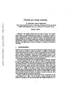
This section discusses how the properties of DCMs are used to simplify their implementation. A key simplification is that actions that have no effect on the agent’s local state are disallowed. This is justified by theorem 6. A second key simplification is that there is no need to worry about race conditions. Thus it is not necessary to ensure that agents wait for each other, or that only one agent is “active” at any given point in time. Given these two simplifications, the implementation of a DCM is as follows: • Each agent has an associated CM module which contains the state (fluents 24
and commitments) local to that agent and updates the CM with the effects of actions (see Figure 5) • At each execution cycle the CM gives the agent the state and a list of enabled actions (those actions that (a) have a true pre-condition; and where (b) executing the action has an effect on the state, i.e. N (X ∪ Ea+ ) 6= X). • The agent then provides the CM with a selected action from the list, or the special “do-nothing” action wait. • The agent’s local CM updates the state by performing the action (Xnew := N (Xold ∪ Ea+ ), since in a monotonic DCM Ea− = ∅) and sends a message to the relevant roles (those in the action’s RI ). If the agent selected the wait action then the state is unchanged and no messages are sent. • When the agent’s CM module receives a message from another agent’s CM module it updates the state with the effects of the relevant action. Note that the only synchronisation required is that within a single CM module changing the state due to an agent’s action and due to a received message does not occur at the same time. There is no need for any synchronisation or coordination between agents. The sequence of events below is one possible execution of the Outrageous Haircut example. The numbers in the left column correspond to the states in Figures 3 and 4. The next two columns show the local state for each of the two agents where the state is given as a number (referring to the states given in Figure 1) and a message queue. The final column gives the change that leads from one row to the next. This change is either an action (e.g. “you : offer”) or processing a message (e.g. “me ← offer”). For example, the first row shows that both agents “me” and “you” start in state 1, and that agent “you” performs the offer action, resulting in row 2 where agent “me” has a message, and agent “you” is in state 2 of Figure 1, i.e. has the conditional commitment CC(you, me, CC(me, you, cutyou, cutme), cutyou). Similarly, the third row is the result of agent “me” performing the accept action
25
which takes it from state 1 of Figure 1 to state 6, i.e. from having no commitments to having the commitment CC(me, you, cutyou, cutme). DCM
Me
You
1
1, hi
1, hi
2
1, hofferi
2, hi
3
6, hofferi
2, haccepti
4
3, hi
2, haccepti
5
3, hi
3, hi
6
3, hcutyoui 4, hi
7
4, hi
4, hi
8
5, hi
4, hcutmei
9
5, hi
5, hi
Change you : offer me : accept me ← offer you ← accept you : cutyou me ← cutyou me : cutme you ← cutme
The following shows another possible execution where agent “you” cuts its hair before the agent “me” realises that an Offer has been made, i.e. agent “me” processes the message offer after agent “you” does the action cutyou. DCM
Me
You
1
1, hi
1, hi
13
6, hi
1, haccepti
3
6, hofferi
2, haccepti
10
6, hofferi
3, hi
11
6, hoffer,cutyoui 4, hi
6
3, hcutyoui
4, hi
7
4, hi
4, hi
8
5, hi
4, hcutmei
9
5, hi
5, hi
26
Change me : accept you : offer you ← accept you : cutyou me ← offer me ← cutyou me : cutme you ← cutme
6
Conclusion
A new formalisation of CMs has been presented. This formalisation is based on the notion of implied commitments and includes a general normalisation operator. As can be seen from the code in appendix A, this formalisation is simpler than previous formalisations such as [12]. This new formalisation was used as the basis for defining Distributed Commitment Machines (DCMs). These are more realistic, since they do not assume a centralised state, and are thus a more suitable basis for implementation. Properties of DCMs were explored, and a number of strong symmetry properties were proven, including the lack of race conditions in monotonic DCMs. These properties rely on symmetries in the handling of commitments, and thus require the axioms of Winikoff et al. [12]: they do not hold for the original CM framework of Yolum and Singh. Finally, an approach for implementing agent interaction using DCMs was described. This approach exploits the symmetry properties to simplify the implementation. In particular, there is no need to worry about race conditions or synchronisation between agents due to the commutativity properties of monotonic DCMs. Although this paper advances the state of the art for commitment-based interaction, there are a number of outstanding issues. What this paper has presented is a theoretical framework which may be simpler, and may address the centralisation problem, but is still just a theoretical framework. For this approach to be used in practice requires that the approach be made pragmatic. Two key missing pieces are a methodology for designing commitment-based interactions, and a guide to mapping an interaction designed as a commitment machine to an implementation. A methodology is needed to guide the software designer in the development of the interaction. It should provide a simple process that assists in determining what commitments are needed and when they should be created. Ultimately, the application of the methodology should result in a commitment machine that will realise the desired interaction, allowing the desired goals of the interaction to be
27
achieved in a range of ways, while preventing the interaction from reaching undesired states. It is also desirable for there to be tool support that assists the designer in developing the interaction and in assuring that it is correct. A specific piece of advice that can be drawn from the work of this paper is that one should strive to create monotonic DCMs. Once an interaction has been designed it needs to be implemented, and there is a need for guidance as to how this should be done. In section 5 an outline of one approach for implementing commitment-based interactions was sketched, but clearly more work is needed to make implementation of commitment-based interactions easy and routine. Compared with other approaches for developing more flexible interactions (discussed in section 1), commitment machines are, in the author’s opinion, not (yet) a pragmatic and usable approach. However, none of the other commitmentbased approaches, nor the landmark-based approach, provide a design methodology, and thus they cannot, at this point in time, be seen as a pragmatic approach for designing flexible interactions. On the other hand, although the work on Hermes [2, 3] is clearly pragmatic, it does not have clear conceptual foundations, nor semantics for its concepts. In addition to the two key areas for future work — methodologies and implementation techniques — there are a number of smaller, but nevertheless important, areas for future work. One of these concerns eliminating redundant messages. When an agent performs an action it sends messages to all agents in RI . It is possible that some of these messages in fact are not needed for the interaction to work. For example, if a Barber agent is added to the Outrageous Haircut example, where the Barber agent receives a request to cut hair from either agent “me” or “you” and does the haircut, then the Barber does not need to know about the negotiations or commitments leading up to the request for a haircut. It should be possible to perform analysis which detects this and automatically derives a simpler local CM for the Barber agent that does not require the Barber agent to be sent unnecessary messages. A second area concerns the restriction to monotonic DCMs. Clearly, it would 28
be desirable to identify more precise conditions that allow DCMs to remain racecondition-free without requiring them to be monotonic. Acknowledgements The author would like to acknowledge the support of Agent Oriented Software Pty. Ltd. and of the Australian Research Council (under grant LP0453486, Advanced Software Engineering Support for Intelligent Agents).
References [1] Rafael H. Bordini, Mehdi Dastani, J¨urgen Dix, and Amal El Fallah Seghrouchni, ed., Multi-Agent Programming: Languages, Platforms and Applications, Springer, 2005. ISBN 0-387-24568-5. [2] Christopher Cheong and Michael Winikoff,
Hermes: Designing goal-
oriented agent interactions, in: Agent-Oriented Software Envineering VI, J. M¨uller and F. Zambonelli, ed., Springer, LNCS 3950, 2006, 16–27. [3] Christopher Cheong and Michael Winikoff, Improving flexibility and robustness in agent interactions: Extending Prometheus with Hermes, in: Software Engineering for Multi-Agent Systems IV: Research Issues and Practical Applications, A. Garcia, R. Choren, C. Lucena, P. Giorgini, T. Holvoet and A. Romanovsky, ed., Springer, LNCS 3914, 2006, 189–206. [4] Roberto A. Flores and Robert C. Kremer, A pragmatic approach to build conversation protocols using social commitments, in: Autonomous Agents and Multi-Agent Systems (AAMAS), N. R. Jennings, C. Sierra, L. Sonenberg, and M. Tambe, ed., ACM Press, 2004, 1242–1243. [5] Nicoletta Fornara and Marco Colombetti, Operational specification of a commitment-based agent communication language, in: Autonomous Agents and Multi-Agent Systems, C. Castelfranchi and W. Lewis Johnson, ed., ACM Press, 2002, 535–542.
29
[6] Marc-Philippe Huget and James Odell, Representing agent interaction protocols with agent UML, in: Agent Oriented Software Engineering V, J. Odell, P. Giorgini, and J. P. M¨uller, ed., Springer, LNCS 3382, 2005, 16–30. [7] Rob Kremer and Roberto Flores, Using a performative subsumption lattice to support commitment-based conversations, in: Autonomous Agents and Multi-Agent Systems (AAMAS), F. Dignum, V. Dignum, S. Koenig, S. Kraus, M. P. Singh, and M. Wooldridge, ed., ACM Press, 2005, 114–121. [8] Sanjeev Kumar and Philip R. Cohen, STAPLE: An agent programming language based on the joint intention theory, in: Autonomous Agents and MultiAgent Systems (AAMAS), N. R. Jennings, C. Sierra, L. Sonenberg, and M. Tambe, ed., ACM Press, 2004, 1390–1391. [9] Sanjeev Kumar, Marcus J. Huber, and Philip R. Cohen, Representing and executing protocols as joint actions, in: Autonomous Agents and MultiAgent Systems, C. Castelfranchi and W. Lewis Johnson, ed., ACM Press, 2002, 543–550. [10] Lin Padgham and Michael Winikoff, Developing Intelligent Agent Systems: A Practical Guide, John Wiley and Sons, 2004. ISBN 0-470-86120-7. [11] Wolfgang Reisig, Petri Nets: An Introduction, Springer-Verlag, 1985. ISBN 0-387-13723-8. [12] Michael Winikoff, Wei Liu, and James Harland, Enhancing commitment machines, in: Declarative Agent Languages and Technologies II, J. Leite, A. Omicini, P. Torroni, and P. Yolum, ed., Springer, LNAI 3476, 2004, 198– 220. [13] Michael Wooldridge, An Introduction to MultiAgent Systems, John Wiley & Sons, 2002. ISBN 0 47149691X.
30
[14] P. Yolum and M.P. Singh, Commitment machines, in: Agent Theories, Architectures, and Languages (ATAL), J-J. Ch. Meyer and M. Tambe, ed., Springer, LNCS 2333, 2002, 235–247. [15] Pınar Yolum, Towards design tools for protocol development, in: Autonomous Agents and Multi-Agent Systems (AAMAS),
F. Dignum, V.
Dignum, S. Koenig, S. Kraus, M. P. Singh, and M. Wooldridge, ed., ACM Press, 2005, 99–105. [16] Pınar Yolum and Munindar P. Singh, Flexible protocol specification and execution: Applying event calculus planning using commitments, in: Autonomous Agents and Multi-Agent Systems, C. Castelfranchi and W. Lewis Johnson, ed., ACM Press, 2002, 527–534. [17] Pınar Yolum and Munindar P. Singh, Reasoning about commitments in the event calculus: An approach for specifying and executing protocols, Annals of Mathematics and Artificial Intelligence (AMAI), 42(1-3) (2004), 227–253.
31
Author Biography Dr. Michael Winikoff is a senior lecturer at RMIT University. His research interests concern notations for specifying and constructing software. Dr. Winikoff received his PhD in 1997 from the University of Melbourne in the area of logic programming with linear logic. He then spent a year and a half as a research fellow at the University of Melbourne working on animating formal specifications. After a stint in the USA (working for the Institute for Software Research) he returned to Australia to join RMIT University’s agent group. In addition to his academic experience Dr. Winikoff has also worked as a consultant for Agent Oriented Software, developers of the JACK agent platform, and has worked as a software developer in industry. These days he is perhaps best known — with Professor Lin Padgham — as the developer of the Prometheus methodology and author of the book Developing Intelligent Agent Systems: A Practical Guide, published by Wiley and Sons in 2004.
32
A
Implementation
The Prolog code below implements the inference rules presented in section 3 and the normalisation process. The code can be obtained from http://www.winikoff. net/CM. implies(X,P) is true if the formula P is implied by state (formula list) X. implies(X,P) :- member(P,X). implies(X,c(P)) :- implies(X,P). implies(X,c(P)) :- member(cc(Q,P),X), implies(X,Q). implies(X,cc(_,Q)) :- implies(X,Q). implies(X,cc(_,Q)) :- implies(X,c(Q)). norm(A,B): B is the normalised form of A. norm(A,B) :- norm(A,A,B). norm(_,[],[]). norm(S,[c(P)|X],R) :- implies(S,P), !, norm(S,X,R). norm(S,[cc(P,Q)|X],R) :not implies(S,Q), implies(S,P), !, R=[c(Q)|R1], norm(S,X,R1). norm(S,[cc(P,Q)|X],R) :(implies(S,Q) ; implies(S,c(Q))), !, norm(S,X,R). norm(S,[P|X],[P|R]) :- norm(S,X,R).
33
offer 1
2
accept offer
accept
3
cutyou
4
cutme
5
6
1=∅ 2 = {CC(you, me, CC(me, you, cutyou, cutme), cutyou)} 3 = {CC(me, you, cutyou, cutme), C(you, me, cutyou)} 4 = {cutyou, C(me, you, cutme)} 5 = {cutyou, cutme} 6 = {CC(me, you, cutyou, cutme)} Figure 1: FSM for non-distributed haircut example, final states are shaded
34
1 send-offer send-accept 2
52
receive-offer send-accept send-offer 50 send-offer
3
receive-offer send-accept
51
receive-offer
receive-accept
4 send-accept send-offer receive-offer
receive-accept
5
53 receive-accept
send-offer
6 receive-accept
send-accept
receive-accept
46 receive-accept send-accept
54
send-cutyou
receive-accept
43
send-accept 7
receive-offer send-offer receive-offer send-offer
send-cutyou
receive-offer
send-accept
44
send-cutyou send-offer
49
47
receive-offer receive-accept
send-cutyou
8
send-accept receive-accept
send-cutyou
send-accept receive-accept
48
receive-offer
send-offer
45
receive-offer receive-offer
send-offer
receive-offer
9 send-cutyou
receive-accept
send-accept 42
receive-cutyou
receive-cutyou
40 send-accept
receive-accept 10
send-cutyou receive-cutyou
receive-cutyou
send-cutyou
send-cutme
35 send-accept
11
receive-accept
send-cutme
send-cutyou
41 send-offer
receive-offer
receive-cutyou
send-cutme
12
send-offer
send-offer
send-cutme
send-offer
receive-offer
37
send-accept receive-accept
send-accept receive-accept
34 send-accept
receive-accept
receive-cutyou
send-cutyou
36 receive-cutyou send-cutyou
33 receive-cutyou send-cutyou
receive-cutme
39 send-offer
send-cutme
send-accept
25
receive-accept
send-offer
send-offer
receive-offer
38
send-offer
receive-offer
receive-accept
send-accept
24
send-cutme
send-cutme
receive-cutme 31
send-cutme
receive-cutyou
send-cutme 19
send-cutyou
send-offer receive-offer
14
18
send-accept send-accept receive-accept
receive-cutyou
13
send-cutyou 17
receive-cutyou send-cutyou
receive-cutme
32
send-cutme
receive-cutme
send-offer
receive-offer
send-cutme
receive-cutme
receive-cutme
22 send-offer
receive-offer receive-cutme
send-accept
receive-accept
send-accept
send-accept
send-accept
send-cutyou
receive-cutyou
15 send-cutyou
receive-cutyou
receive-cutme
receive-cutme
send-cutme
send-cutme
16 receive-cutme
send-cutyou
receive-cutyou
receive-cutyou send-cutyou
send-cutyou receive-cutyou
send-cutyou receive-cutyou 29
send-offer
receive-cutme
send-cutme
30 receive-accept
send-offer send-offer
send-offer
receive-offer
send-offer 26
send-accept
receive-cutyou send-cutyou
23
27 send-cutme receive-cutme 28 receive-accept
send-accept
send-accept
21 send-cutme receive-cutme 20
Figure 2: Complex FSM resulting from distributing the simple CM (Note that this figure is not meant to be legible, but to illustrate the complexity of the resulting FSM which has 54 states and 164 transitions).
35
1 send-offer send-accept 2
13
receive-offer send-accept send-offer 12
receive-accept
3 send-accept
14
receive-offer
4
receive-accept
send-offer
10 receive-accept receive-offer send-cutyou 5
11 send-cutyou receive-offer 6 receive-cutyou 7 send-cutme 8 receive-cutme 9
Figure 3: Simpler FSM resulting from preventing actions that have no local effect, final states are shaded
36
1. {me 7→ h{}, hii, you 7→ h{}, hii} 2. {me 7→ h{}, hoffer ii, you 7→ h{CC(you, me, CC(me, you, cutyou, cutme), cutyou)}, hii} 3. {me 7→ h{CC(me, you, cutyou, cutme)}, hoffer ii, you 7→ h{CC(you, me, CC(me, you, cutyou, cutme), cutyou)}, hacceptii} 4. {me 7→ h{CC(me, you, cutyou, cutme), C(you, me, cutyou)}, hii, you 7→ h{CC(you, me, CC(me, you, cutyou, cutme), cutyou)}, hacceptii} 5. {me 7→ h{CC(me, you, cutyou, cutme), C(you, me, cutyou)}, hii, you 7→ h{CC(me, you, cutyou, cutme), C(you, me, cutyou)}, hii} 6. {me 7→ h{CC(me, you, cutyou, cutme), C(you, me, cutyou)}, hcutyouii, you 7→ h{cutyou, C(me, you, cutme)}, hii} 7. {me 7→ h{cutyou, C(me, you, cutme)}, hii, you 7→ h{cutyou, C(me, you, cutme)}, hii} 8. {me 7→ h{cutyou, cutme}, hii, you 7→ h{cutyou, C(me, you, cutme)}, hcutmeii} 9. {me 7→ h{cutyou, cutme}, hii, you 7→ h{cutyou, cutme}, hii} 10. {me 7→ h{CC(me, you, cutyou, cutme)}, hoffer ii, you 7→ h{CC(me, you, cutyou, cutme), C(you, me, cutyou)}, hii} 11. {me 7→ h{CC(me, you, cutyou, cutme)}, hoffer , cutyouii, you 7→ h{cutyou, C(me, you, cutme)}, hii} 12. {me 7→ h{CC(you, me, CC(me, you, cutyou, cutme), cutyou)}, hii, you 7→ h{CC(you, me, CC(me, you, cutyou, cutme), cutyou)}, hii} 13. {me 7→ h{CC(me, you, cutyou, cutme)}, hii, you 7→ h{}, hacceptii} 14. {me 7→ h{CC(me, you, cutyou, cutme)}, hii, you 7→ h{CC(me, you, cutyou, cutme)}, hii} Figure 4: Details on the states in the FSM of Figure 3
37
CM module
CM module
Agent A
Agent B
Figure 5: Execution Model (showing two agents)
38