Hindawi Publishing Corporation International Journal of Distributed Sensor Networks Volume 2015, Article ID 828906, 13 pages http://dx.doi.org/10.1155/2015/828906
Research Article Implementing PMIPv6 Protocol Based on Extended Service Set for IEEE 802.11 Infrastructure WLAN Deqing Zhu,1,2 Lin Xu,3 Yi-hua Zhu,1 and Xianzhong Tian1 1
School of Computer Science and Technology, Zhejiang University of Technology, Hangzhou, Zhejiang 310023, China Education Technology Center of Hangzhou Normal University, Hangzhou, Zhejiang 310018, China 3 Institute of Information Intelligence and Decision Optimization, Zhejiang University of Technology, Hangzhou, Zhejiang 310023, China 2
Correspondence should be addressed to Yi-hua Zhu;
[email protected] Received 18 December 2014; Accepted 19 January 2015 Academic Editor: Xiuzhen Cheng Copyright © 2015 Deqing Zhu et al. This is an open access article distributed under the Creative Commons Attribution License, which permits unrestricted use, distribution, and reproduction in any medium, provided the original work is properly cited. With the popularity of IEEE 802.11 based wireless fidelity (Wi-Fi) portable devices, it becomes increasingly significant to support the mobile users carrying Wi-Fi devices to access the Internet of Things (IoT) so that the communications between the mobile users and the smart objects deployed in the IoT stay uninterrupted when the mobile users are in movement. A scheme using Extended Service Set- (ESS-) based architecture is presented to implement the proxy mobile IPv6 protocol, that is, PMIPv6, for IEEE 802.11 infrastructure Wireless Local Area Networks (WLANs). The key signaling packets together with their time sequences for the mobility management in the proposed scheme are proposed. Moreover, the handoff delay in the proposed scheme is derived, through which the performance of the proposed scheme is analyzed. Numerical analysis indicates that the proposed scheme considerably outperforms the existing scheme that uses the Basic Service Set (BSS) based architecture in terms of handoff delay in the case when the delay between Mobile Access Gateway (MAG) and local mobile anchor (LMA) is relatively large.
1. Introduction Wireless Local Area Network (WLAN) interfaces or Wi-Fi are increasingly incorporated in multimedia portable electronic devices such as portable computers and smart phones. These interfaces enable these devices to access the Internet wherever WLAN Access Points (APs) are located. Most IEEE 802.11 WLANs operate in the infrastructure mode, in which each node is associated with an AP to access the Internet [1]. In Internet of Things (IoT), it is required to attach IP addresses to everyday objects allowing people to remotely communicate with and control networked devices. Having the advantages of easy integration with existing infrastructure, built-in IP-network compatibility, and familiar protocols and management tools [2], Wi-Fi enabled sensors have been used in IoT [3–5]. The Wi-Fi enabled sensors have the feature of at least two wireless interfaces: one is the Wi-Fi interface used to access IEEE 802.11-based WLAN and the other is the low-power interface to support IEEE 802.15.4 standard.
Thus, data packets can be transmitted with high data-rate via the Wi-Fi interface while the communications between lowpower devices go through the low-power interface [1]. Nowadays, Wi-Fi enabled portable smart phones equipped with some sensors have become increasingly popular. For example, the Samsung Galaxy smart phone includes more than 10 kinds of sensors, such as temperature and humidity sensors, accelerometer, and gyroscope, and so forth. Many applications have been developed to use the sensors embedded in the smart phones, in which the data collected by the embedded sensors from the environment are transmitted via the Wi-Fi interface connecting to the AP in the WLAN. Internet Protocol Version 6 (IPv6) [6], which has been widely used in the Internet, was applied in wireless sensor networks (WSNs). For instance, IPv6 was used in the WSN for ambient monitoring [7]; the double adaptively clustering hierarchy (DACH) algorithm used IPv6 in WSN [8]; and IPv6-based all-IP WSNs were investigated in [9]. To support delivering IPv6 packets over low-power and low-rate WSNs,
2
International Journal of Distributed Sensor Networks
6LoWPAN protocol [10] was developed by the Internet Engineering Task Force to enable nodes in the IP network to communicate with the low-powered WSN nodes operating at low data rates [11]. The adaptation layer introduced in 6LoWPAN is located between the medium access (MAC) layer and the network layer in the protocol stack [10]. With the rapid growth in the number of portable electronic devices, it becomes urgent to support the users carrying these devices to access the IoT when the users are moving, which inspirits researchers to investigate the problem of implementing mobile IPv6 (MIPv6) in the infrastructure WLANs. MIPv6 is a technology which allows users to stay connected to the Internet when they are moving. MIPv6 protocols can be classified into two categories: the host-based protocol, such as MIPv6 [12] and HMIPv6 [13]; and the network-based protocol, such as PMIPv6 [14]. IEEE 802.11 standard supports link-layer mobility; that is, it supports mobile node (MN) to move across the boundary of radio coverage of an AP within the same WLAN. But, it does not support network-layer mobility [15], which supports the MN to move across an IP subnet. As a result, we need the network layer mobility protocol that supports the MN to seamlessly move in different WLANs such that the MN keeps its ongoing communications uninterrupted when moving across the boundary of IEEE 802.11 WLANs. Considering that the PMIPv6 has many advantages (e.g., MNs are free from handling mobility management), Gundavelli [16] presented in 2010 the idea of implementing PMIPv6 protocol in WLANs. Unfortunately, this idea has not been finalized as a standard up to date although it has undergone six times of improvements [17]. There are two core functional entities in PMIPv6 protocol. That is, the local mobility anchor (LMA) and the Mobile Access Gateway (MAG). According to Gundavelli’s suggestion, relationship between MAG and AP can be as follows: (1) a MAG manages only one AP, referred to as single AP architecture” below; and (2) a MAG manages more than one AP, referred to as “multi-AP architecture” below. In 2012, Chai et al. [18] proposed a scheme to implement PMIPv6 for single AP architecture. To the best of our knowledge, there is still a lack of the implementation scheme for multi-AP architecture, which motivates us to address the problem. We extend our previous research [19] in this paper, which has the main contributions as follows. (1) A novel scheme to implement PMIPv6 using Extended Service Set (ESS) based architecture, that is, ESS-based architecture, is presented. (2) The signaling commands used in mobility management and their timing diagrams for the proposed scheme are designed. (3) Delay and signaling traffic in the proposed scheme are derived, based on which performance analysis is conducted. The remainder of this paper is organized as follows. Our scheme is presented in Section 2 and performance analysis is given in Section 3. We conclude the paper in Section 4.
Internet
LMA IP network
BSS4 MAG4 /AP4 MAG1 /AP1
MAG2 /AP2
MN BSS1
BSS2
MAG3 /AP3
BSS3
Figure 1: The BSS-based architecture.
2. Implementing PMIPv6 Using ESS-Based Architecture In PMIPv6 protocol, LMA and MAG manage mobility on behalf of an MN, releasing the MN from the burden of handling mobility-related signaling. LMA maintains the MN’s home network prefix (HNP) and records entries relevant to the associations between MAG and MN, and it acts as the home agent (HA) of the MN, while MAG is used to detect the MN’s movement and reports its current position to LMA when necessary. A packet destined to the MN from corresponding node (CN) is first delivered to its LMA using IP protocol and then, via the tunnel between the LMA and the MAG, the packet is tunneled to the MN’s MAG through which it is delivered to the MN using the point-to-point link between the MN and the MAG. Compared to MIPv6, HMIPv6, and the other host-based mobility management protocols, PMIPv6 has the following advantage in addition to saving bandwidth [20]: mobility management is transparent to the MN (i.e., the MN is not involved in mobility management). This strength frees the MN from installing or updating the software to support mobility. Thus, PMIPv6 is highly likely to be widely used. 2.1. The ESS-Based Architecture. In an infrastructure IEEE 802.11 WLAN [15], nodes access the Internet via an AP and the radio coverage of the AP is known as basic service area (BSA). Each node must be associated with one AP before joining the WLAN. The AP and all its associated MNs form a Basic Service Set (BSS) and multiple BSSs form an Extended Service Set (ESS). The key to implement PMIPv6 in WLAN lies in handling the relationship between MAG and AP. That is, how many APs should be managed by a single MAG. The structure in which one MAG manages only one AP (i.e., the MAG manages one BSS) is illustrated in Figure 1, where each AP is collocated with a MAG. This structure will be referred to as BSS-based architecture below. In this paper, we present the ESS-based architecture shown in Figure 2, where a MAG manages an ESS containing multiple APs. For the sake of easy
International Journal of Distributed Sensor Networks
Internet
LMA IP network
MAG2 /AP8
MAG1 /AP1
AP10 AP2
AP3
AP4
AP5
AP6
AP7
AP9 AP11
MN ESS1
ESS2
Figure 2: The ESS-based architecture.
3 in active scanning. Hence, in this paper, we assume that the MN uses active scanning to detect APs. After scanning, the MN has obtained all necessary information including MAC addresses and signal strengths of the scanned APs, which enable the MN to choose a desired AP to associate with. The MN judges whether it has entered the area of a new ESS by comparing its buffered service set identifier (SSID) with the SSID carried in the received beacon frame. Before association with a new AP, authentication is needed to verify the identity of the MN. In the case when open system authentication is in use, only one set of authentication request (AuReq) and response (AuRes) exchange suffices for the authentication process [21]. After that, the MN is associated with the new AP by exchanging reassociation request (RAReq) and response (RARes). Considering the above handoff process is only involved in MAC layer, we call it “L2 handoff.” The events occurring after L2 handoff are as follows. (1) Association with an AP in Different ESS. In this case, the MN sends a router solicitation message (RtrSol) to the MAG. After receiving RtrSol, the MAG sends a PBU to the LMA. Once the LMA accepts the PBU, it sends back to the MAG a proxy binding acknowledgment (PBA) message, which contains the MN’s home network prefix option, and then it sets up a route over the tunnel to the MAG. After successfully receiving the PBA, the MAG sends router advertisement message (RtrAdv), from which the MN constructs its IP address using the carried HNP. The above process happens in network layer, which will be referred to as “L3 handoff ” in the sequel. The events involved in the L2 and L3 handoffs are illustrated in Figure 3. Furthermore, the signaling exchanges among the MN, the new AP, the MAG-AP, and the LMA are shown in Figure 4(a). There exists an exception that happens when the new AP is also a MAG-AP such that the signaling exchanges of RtrSol and RtrAdv can be omitted, which is shown Figure 4(b).
description, an AP that is collocated with a MAG is called a “MAG-AP” hereinafter. Thus, in Figure 1, each AP is a MAGAP; whereas, in Figure 2, only one of the APs in the same ESS is chosen as MAG-AP (e.g., AP1 and AP8 are MAG-APs). In both architectures, all APs are wiredly connected. In the BSS-based architecture, whenever an MN crosses the boundary of a BSA, a handoff operation is triggered, which sends a proxy binding update (PBU) message to the LMA from the MAG in order to update the MN’s new location [14]. For example, in Figure 1, when the MN moves from the BSA of AP1 to that of AP2 , the MAG related to AP2 sends a PBU message to the LMA. In the proposed ESSbased architecture, a PBU message is sent only when the MN goes across the boundary of the radio coverage of the ESS. Moreover, when the MN moves within the radio coverage of the same ESS, no PBU message is needed no matter how many BSAs are crossed. For instance, when the MN moves from the BSA of AP3 to that of AP4 , no PBU is needed. But, when the MN moves from the BSA of AP4 to that of AP5 , the MAG collocated with AP8 (i.e., MAG2 ) sends a PBU to the LMA. In the proposed scheme, in every MAG-AP, a cache called “AssocTable” is set to record the information of current APs of MNs. AssocTable contains two fields: “MN ID” and “Curren AP,” which are used to save the MN’s unique identifier and the currently associated APs, respectively.
(2) Association with AP in the Same ESS. In this case, the MN neither sends a RtrSol message nor updates its IP address. The only thing it needs to do is to let the new AP inform the MAG-AP of updating its AssocTable. The events in this case are shown in Figure 5. Additionally, the signaling exchanges among the MN, the new AP, and the MAG-AP are illustrated in Figure 6(a), in which the UAT-Req and UATACK represent the message of updating AssocTable and the acknowledgement, respectively.
2.2. Mobility Management Strategy for the ESS-Based Structure. In infrastructure WLAN, the MN uses active scanning or passive scanning to find existing networks in the area. With active scanning, the MN sends probe frames to solicit responses instead of awaiting the announcement of the network. With passive scanning, the MN searches in each of the preset channels for at least a beacon interval (BI) to receive a possible beacon frame from an AP. The default value of BI is 0.1 s. Therefore, the time consumed in passive scanning can be up to a couple of seconds, which is far greater than that
2.3. Other Specifications. The MAG acts as the default router of the MN and emulates the MN’s home link [14]. As a mobility entity, the MAG can access the policy profile of the MN, which includes a set of configuration parameters for the MN. When PMIPv6 is implemented in an infrastructure WLAN, the configuration parameters such as the MN’s identifier and the LMA address can be piggybacked in association request message, thus saving the time required to access the policy profile. Apart from the MN’s static HNP in the policy profile, the MAG can get a dynamically allocated HNP from PBA
4
International Journal of Distributed Sensor Networks tL2
tBU
Scanning Authentication Reassociation RtrSol PBU PBA MAG sends RtrAdv IP address Time configuration L2 handoff ends L2 handoff L3 handoff ends (L3 handoff starts) trigger
Figure 3: Events in L2 and L3 handoffs.
MN
MAG-AP
AP
LMA
Scanning
LMA
MAG-AP
MN Scanning
Authentication starts Authentication end
Authentication starts Authentication end
RAReq
RAReq
RARes RtrSol
RARes PBU PBA
RtrAdv
PBU PBA
IP address configuration
IP address configuration (a) When the new AP is not a MAG-AP
(b) When the new AP is a MAG-AP
Figure 4: Signaling exchanges when the MN crosses the boundary of an ESS.
tL2
Scanning L2 handoff trigger
Authentication
tUAT Reassociation
Update AssocTab in the MAG-AP
L2 handoff ends
Time IP address configuration
Figure 5: Events when MN moves in the same ESS.
message. With the HNP and its identifier in hands, the MN can use stateless address configuration method to build its IP address. In the infrastructure IEEE 802.11 WLAN, upon receiving a frame destined to the MN, the AP uses the distribution service provided by the distribution system to deliver the frame to MN. But, IEEE 802.11 standard does not specify how to implement the distribution system. In this paper, the APs in an ESS are wiredly connected to form the distribution system. When a frame from the wired network is forwarded to the 802.11 WLAN, its format has to be converted before it is delivered to the MN [15]. In addition, some mobility signaling messages sent by the MN should be treated as a new kind of control messages defined according to IEEE 802.11 standard. For example, following IEEE 802.11 standard, we assign new control frame subtype values of “0001” and “0010” in the header of IEEE 802.11 MAC frame for the RtrSol and RtrAdv messages, respectively. In PMIPv6, the Access Technology Type option is mandatory. We set it to 4, which means that the access technology is 802.11 [14].
3. Performance Analysis 3.1. Handoff Delay. In this section, we use handoff delay as a metric to compare our scheme that uses the ESS-based architecture shown in Figure 2 with the BSS-based architecture shown in Figure 1. Similar to [22], we use a square to represent a BSS. As shown in Figure 7, each small square represents a BSS and several small squares constitute a big square with bold box to represent an ESS. The MN in a BSS is allowed to move into any of the 8 adjacent BSSs. The lower left corner in Figure 7 shows the 8 possible moving directions if the MN is located in square 𝑋. Noting that an ESS is formed by 𝑛×𝑛 adjacent squares with each standing for a BSS, the ESS contains 𝑛2 BSSs. In Figure 7, letter “𝐶” represents the MN in the corner of an ESS, letter “𝐵” indicates the MN in the edges rather than the corner of an ESS, and letter “𝐼” represents the MN in the inner of an ESS. Then, the probabilities of the MN in the BSSs labeled with letters “𝐶,” “𝐵,” and “𝐼” are, respectively, as follows: 𝑎𝐶 =
4 ; 𝑛2
𝑎𝐵 =
4 (𝑛 − 2) ; 𝑛2
𝑎𝐼 =
𝑛2 − 4 (𝑛 − 1) (1) . 𝑛2
International Journal of Distributed Sensor Networks
AP
MN Scanning
5
MAG-AP
MAG-AP
MN Scanning
Authentication starts
Authentication starts
Authentication end
Authentication end
RAReq
RAReq
RARes
RARes
UAT-Req
UAT-ACK (a) When the new AP is not a MAG-AP
(b) When the new AP is a MAG-AP
Figure 6: Signaling exchanges when MN moves in the same ESS.
C
B
B
B
C
B
I
I
I
B
B
I
I
I
B
B
I
I
I
B
C
B
B
B
C
is newly associated with when the MN enters a new BSS) is a MAG-AP is 1/𝑛2 and (2) when the MN does not cross the border of ESS0 (with probability 3/8), the probability that the new AP is a MAG-AP, which occurs only when the MN is not located in MAG-AP (with probability (𝑛2 − 1)/𝑛2 ), is [(𝑛2 − 1) / 𝑛2 ] × 1/(𝑛2 − 1) = 1/𝑛2 . Thus, when the MN is located at the corner, the probability that the MN moves into an area of a MAG-AP is equal to 𝑎𝐶 [(5/8)(1/𝑛2 ) + (3/8)(1/𝑛2 )] = 𝑎𝐶× 1/𝑛2 . n
X
n
Figure 7: BSS with small square and ESS with bold square.
When the MN is at the corner of an ESS (refer to the BSS labeled with letter “𝐶” in Figure 7), the probability that the MN also crosses the boundary of the ESS when it crosses a BSS is 5/8; when the MN is in the BSS with “𝐵,” the probability of ESS boundary-crossing is 3/8; and when the MN is within an ESS, the probability of ESS boundary-crossing is 0 as it does not cross the boundary of an ESS when the MN crosses a BSS. Thus, the probability that the MN crosses the boundary of an ESS after the MN crosses a BSS is 3 3𝑛 − 1 5 . 𝑝 = 𝑎𝐶 + 𝑎𝐵 = 8 8 2𝑛2
(2)
Let 𝑞0 be the probability that the MN moves from a BSS to the coverage of a MAG-AP. Now, we calculate 𝑞0 . Assume that the MN is currently in ESS0 (see Figure 8). After one BSS boundary crossing, the MN enters a new BSS (i.e., a new AP), which leads to the following three cases according to whether the MN has crossed the boundary of ESS0 or not. Case 1. The MN is currently located at the corner of ESS0 as shown in Figure 8(a). There are two subcases for Case 1: (1) when the MN crossed the boundary of ESS0 (with probability 5/8), the probability that the new AP (i.e., the AP the MN
Case 2. The MN is currently located at edge “𝐵” as shown in Figure 8(b). Similarly, we can obtain the probability that the MN moves into an area of a MAG-AP is 𝑎𝐵 × 1/𝑛2 . Case 3. The MN is currently located at inner “𝐼” as the square with “𝑋” shown in Figure 7. In this case, only when the MN is not in a MAG-AP, that is, the MAG-AP is collocated with one of the other 𝑛2 − 1 APs, can the MN enter the area of a MAG-AP. Thus, the probability that the MN moves into an area of a MAG-AP is 𝑎𝐼 × [(𝑛2 − 1)/𝑛2 ] × 1/(𝑛2 − 1) = 𝑎𝐼 × 1/𝑛2 . In summary, no matter where the MN is located in ESS0 , the probability that the MN moves into an area of a MAGAP is the sum of the probabilities derived in the above three cases, which equals (3) using (1). Consider 𝑞0 = 𝑎𝐶
1 1 1 1 1 + 𝑎𝐵 2 + 𝑎𝐼 2 = 2 (𝑎𝐶 + 𝑎𝐵 + 𝑎𝐼 ) = 2 . 𝑛2 𝑛 𝑛 𝑛 𝑛
(3)
Let 𝐷ESS be the expected handoff delay in the proposed scheme, that is, the ESS-based architecture shown in Figure 2. From the mobility management strategy presented in Section 2.2, L2 handoff definitively occurs regardless of whether the MN crosses a BSS or not. Further, if the MN crosses the boundary of a ESS and enters the area of a MAGAP, the events of PBU, PBA, and IP address configuration follow (see Figure 4(b)); if the new AP with which the MN is associated is not a MAG-AP, L3 handoff takes place (see Figures 3 and 4(a)). If the MN does not cross the boundary of an ESS, that is, the MN moves within the ESS, when the new AP is a MAG-AP, only L2 handoff happens (see Figure 6(b)); otherwise, UAT-Req and UAT-ACK messages are exchanged
6
International Journal of Distributed Sensor Networks
ESS3
C
ESS2
B
C
B
B
B ESS0
B
B
ESS1
ESS0
B C
C
ESS1
B B
(a) When the MN is located in one of the corners of the ESS
B
B
B
(b) When the MN is located in one of the boundaries of the ESS
Figure 8: The cases of the MN’s crossing a BSS.
(see Figures 5 and 6(a)). As a result, the expectation of handoff delay can be calculated as 𝐷ESS = 𝑝 [𝑞0 (𝑡𝐿2 + 𝑡PBU + 𝛿 + 𝑡PBA + 𝛿)
𝐷ESS =
+ (1 − 𝑞0 ) (𝑡𝐿2 + 𝑡BU )] + (1 − 𝑝) [𝑞0 𝑡𝐿2 + (1 − 𝑞0 ) (𝑡𝐿2 + 𝑡UAT )]
UAT-ACK can be omitted. Thus, using (2) and (3), (4) can be simplified as
(4)
= 𝑝𝑞0 (𝑡PBU + 𝑡PBA + 2𝛿) + 𝑝 (1 − 𝑞0 ) 𝑡BU
3𝑛 − 1 (𝑡PBU + 𝑡PBA + 2𝛿) 2𝑛4 +
(3𝑛 − 1) (𝑛2 − 1) 2𝑛4
(6) 𝑡BU + 𝑡𝐿2 .
+ 𝑡𝐿2 + (1 − 𝑝) (1 − 𝑞0 ) 𝑡UAT , where 𝛿 is the propagation delay between the MAG and the LMA and the time of configuring IP address is ignored. Obviously, the BSS-based architecture shown in Figure 1 is a special case of the ESS-based architecture shown in Figure 2 when 𝑛 = 1. As a result, letting 𝑛 = 1 in (2) and (3), we obtain 𝑝 = 1 and 𝑞0 = 1. Thus, from (4), we obtain that the expected handoff delay in the BSS-based architecture is 𝐷BSS = 𝑡PBU + 𝑡PBA + 𝑡𝐿2 + 2𝛿.
(5)
It can be seen from (4) and (5) that the key to finding 𝐷ESS and 𝐷BSS lies in determining 𝑡PBU , 𝑡PBA , 𝑡BU , 𝑡UAT , and 𝑡𝐿2 . Since UAT-Req and UAT-ACK are sent in wired link, their propagation speeds are as high as 2 × 10⁸ m/s such that the propagation only takes 5 𝜇s if the distance between the AP and the MAG-AP is 1 km. Besides, the payload of UAT-Req or UAT-ACK is only 1 B, which totals 33 B when the 802.11 MAC header is taken into account. Hence, the delay in transmitting UAT-Req or UAT-ACK is less than 3 𝜇s in 100 Mbps Ethernet, which reduces to 0.3 𝜇s in a Gigabit Ethernet. Therefore, the propagation and transmission delay of UAT-Req and
IEEE 802.11 standard lets the nodes adopt the mechanism of distributed coordination function (DCF) in competing for the channel. The CSMA/CA mechanism is used to avoid packet collisions. A node picks a random backoff value 𝑤 in set {0, 1, 2, . . . , CW}. After waiting for the time period of 𝑤𝜎, the data frame is sent, where 𝜎 is the length of a time slot. In addition, the contention window CW ∈ [CWmin , CWmax ], and CW has the initial value of CWmin . Here, CWmin and CWmax are constants that closely depend on which physical layer is in use [4]. If a packet transmission is not successful, then CW = Min{2(CW + 1) − 1, CWmax }; otherwise, CW = CWmin . Therefore, for a given packet, averagely, the node has to wait with the period of 𝜎 (CWmin /2) for the channel in order to transmit the packet. If the first transmission trial fails, then the average waiting time for a retransmission is 𝜎 [2(CWmin + 1) − 1]/2. If the first two trials are not successful, the average waiting time becomes 𝜎 [22 (CWmin + 1) − 1]/2 for the third transmission retrial. Similarly, if the first three consecutive trials are unsuccessful, the waiting time turns to 𝜎 [23 (CWmin + 1) − 1]/2 for the fourth trial. Considering that the probability of the failures of three consecutive transmissions is small, we ignore the failure probabilities of three or more consecutive transmissions. Thus, the average waiting time for
International Journal of Distributed Sensor Networks
7
Table 1: Delay of signaling frames. Frame type PBU RtSol RAReq AuReq UAT-Req
Length (B) 96 72 56 34 35
Transmission delay (𝜇s) 𝑡PBU = 76.8 𝑡RS = 57.6 𝑡RAReq = 44.8 𝑡AuReq = 27.2 𝑡UAT-Req = 28
a node to gain the channel in transmitting a packet can be calculated as 𝑡𝑐 = 𝑝𝑠 𝜎
=𝜎
= 2 (𝑡DIFS + 𝑡𝐶) + 𝑡AuRes + 𝑡AuReq ; (7)
(10)
𝑡𝐿2 = 𝑡Scan + 𝑡Authen + 𝑡RAssoc = 4𝑡𝐶 + 𝑡AuRes + 𝑡AuReq + 𝑡RAReq + 𝑡RARes
4CWmin + 3 + (1 − 𝑝𝑠 ) 𝜎 , 2 2
(11)
+ 𝑡Scan + 4𝑡DIFS .
where 𝑝𝑠 is the probability of successfully transmitting a packet. Let 𝜃 be the probability of successful packet transmitting (PSPT) over the wireless link between the MN and an AP. As positive acknowledgement is applied in IEEE 802.11 WLAN, a transmission failure means that either packet transmission fails or the ACK message is lost. Thus, 𝑝𝑠 = 𝜃2 , which turns (7) into
4CWmin + 3 + (1 − 𝜃 ) 𝜎 . 2
𝑡RAssoc = (𝑡DIFS + 𝑡𝐶 + 𝑡RAReq ) + (𝑡DIFS + 𝑡𝐶 + 𝑡RARes )
From Figures 3 and 5, (10), and Table 1, we have
2CWmin + 1 CWmin + (1 − 𝑝𝑠 ) 𝜎 2 2
2 2
(9)
= 2 (𝑡DIFS + 𝑡𝐶) + 𝑡RAReq + 𝑡RARes .
22 (CWmin + 1) − 1 } 2
CWmin 2CWmin + 1 𝑡𝑐 = 𝜎 + (1 − 𝜃2 ) 𝜎 2 2
Considering that 𝑡Scan is in the range of 105∼210 ms [24], we set 𝑡Scan = 150 ms = 150000 𝜇s. Thus, (8) turns into
𝑡Authen = (𝑡DIFS + 𝑡𝐶 + 𝑡AuRes ) + (𝑡DIFS + 𝑡𝐶 + 𝑡AuReq )
+ (1 − 𝑝𝑠 ) (1 − 𝑝𝑠 )
+𝜎
Transmission delay (𝜇s) 𝑡PBA = 76.8 𝑡RA = 67.2 𝑡RARes = 32 𝑡AuRes = 27.2 𝑡UAT-ACK = 28
Before transmitting, the node must sense the medium idle for period of 𝑡DIFS and then backoffs. Thus, we get
2 (CWmin + 1) − 1 CWmin ⋅ {𝜎 +𝜎 } 2 2
2 (CWmin + 1) − 1 CWmin +𝜎 2 2
Length (B) 96 84 40 34 35
𝑡𝑐 = 1270𝜃4 − 3170𝜃2 + 2210.
CWmin + (1 − 𝑝𝑠 ) 𝑝𝑠 2
⋅ {𝜎
Frame type PBA RtAdv RARes AuRes UAT-ACK
Using Table 1 and (9), we obtain 𝑡𝐿2 = 4𝑡𝐶 + 150331.2 = 5080𝜃4 − 12680𝜃2 + 159171.2. (12) From Figure 3, we have 𝑡BU = (𝑡DIFS + 𝑡𝐶 + 𝑡RS ) + (𝑡PBU + 𝛿) + (𝑡PBA + 𝛿) + (𝑡DIFS + 𝑡𝐶 + 𝑡RA )
(13)
= 2𝑡𝐶 + 2𝑡DIFS + 𝑡RS + 𝑡PBU + 𝑡PBA + 𝑡RA + 2𝛿. From Table 1 and (9), we have
(8)
The peak data rates that IEEE 802.11𝑎/𝑏/𝑔 supports are 54/11/54 Mbps, respectively. Due to environmental interference, multipath fading, and other factors, the theoretical peak data rate cannot be reached in practice. Therefore, we set data rate to 10 Mbps, which generates the transmission delays of various signaling frames in the proposed scheme as shown in Table 1. The frame lengths are the same as those in [15, 23], and delay is calculated from frame length divided by the data rate (i.e., 10 Mbps). Assume that the physical layer of WLAN applies direct sequence spread spectrum (DSSS). According to [15], we set 𝜎 = 20 𝜇s, short frame interval 𝑡SIFS = 10 𝜇s, DCF frame interval 𝑡DIFS = 𝑡SIFS + 2𝜎 = 50 𝜇s, 𝑎CWmin = 31, and 𝑎CWmax = 1023.
𝑡BU = 2𝑡𝐶 + 378.4 + 2𝛿 = 2540𝜃4 − 6340𝜃2 + 4798.4 + 2𝛿.
(14)
Thus, using (12) and (14), (6), and (5) can be rewritten as follows: 3𝑛 − 1 𝐷ESS = (153.6 + 2𝛿) 2𝑛4 +
(3𝑛 − 1) (𝑛2 − 1) 2𝑛4
(15)
⋅ (2540𝜃4 − 6340𝜃2 + 4798.4 + 2𝛿) + (5080𝜃4 − 12680𝜃2 + 159171.2) 𝐷BSS = 5080𝜃4 − 12680𝜃2 + 159324.8 + 2𝛿.
(16)
8
International Journal of Distributed Sensor Networks 𝛿 = 0.5 ms
𝛿 = 0.5 ms
1000
500
500 Δ(n) (𝜇s)
Δ(n) (𝜇s)
1000
0 −500 1
0 0.8 𝜃
10
0.6 0.4
0
5
15
20
n −500
Figure 9: Influence of 𝑛 and 𝜃 on Δ(𝑛).
4
6
8
10
12 n
14
16
18
20
𝜃 = 0.4 𝜃 = 0.6 𝜃 = 0.8
Figure 10: Influence of 𝑛 on Δ(𝑛) when 𝜃 is fixed.
Further, the difference of (5) and (6) is Δ (𝑛) ≡ 𝐷BSS − 𝐷ESS 3𝑛 − 1 = 153.6 + 2𝛿 − (153.6 + 2𝛿) 2𝑛4 (17)
2𝑛4
⋅ (2540𝜃4 − 6340𝜃2 + 4798.4 + 2𝛿) , where “≡” is used to define the notation on its left side, that is, Δ(𝑛), which is expressed as its right side. It can be seen from (17) that, the condition that our scheme using the ESSbased architecture is better than the BSS-based architecture is Δ(𝑛) > 0. Next, we investigate influence of 𝑛, 𝜃 and 𝛿 on Δ(𝑛). The influence for the case when 𝛿 = 1 ms is shown in Figure 9, which indicates that: (1) a larger 𝑛 or 𝜃 cause Δ(𝑛) > 0, that is, our scheme outperforms the BSS-based scheme in terms of delay in the case when more APs are included in an ESS or when the PSPTs over wireless links are larger; and (2) the increase either in 𝑛 or 𝜃 causes Δ(𝑛) to increase, that is, as the PSPTs over wireless links increase or more APs are added to an ESS, the delay difference between the BSS-based architecture and our scheme becomes increasingly apparent, that is, our scheme is better than the BSS-based scheme considerably. To clearly observe the tendency of Δ(𝑛) when 𝑛 and 𝜃 vary, we plot the cross sectional views of Figure 9 in Figures 10 and 11. Figure 10 shows the case when 𝜃 are fixed to 0.2, 0.5, and 0.8, and Figure 11 shows the case when 𝑛 are fixed to 2, 6, 11, 16, and 20. Both figures clearly illustrate that our scheme prefers a larger 𝑛 such that Δ(𝑛) > 0. Moreover, in the case where
500 Δ(n) (𝜇s)
−
(3𝑛 − 1) (𝑛2 − 1)
𝛿 = 0.5 ms
1000
0
−500 0.4
0.45
0.5
0.55
0.6
0.65
0.7
0.75
0.8
0.85
0.9
𝜃 n=4 n=8 n = 12
n = 16 n = 20
Figure 11: Influence of 𝜃 on Δ(𝑛) when 𝑛 is fixed.
PSPSs of wireless links are small, we can choose a larger 𝑛 such that Δ(𝑛) > 0 (see Figure 11). Influence of 𝛿 on Δ(𝑛) is shown in Figure 12, from which we observe that (1) Δ(𝑛) increases proportionally with the propagation delay between the LMA and the MAG (i.e., the parameter 𝛿) and (2) a larger 𝛿 contributes a larger Δ(𝑛). In other words, our scheme considerably outperforms the BSSbased one in the case when 𝛿 is relatively large.
International Journal of Distributed Sensor Networks
9 sending a UAT message. In the case when 𝑛 = 1, we have 𝑝 = 1 and 𝑞0 = 1 from (2) and (3). Thus, from (19), we get the expected handoff traffic for the BSS-based architecture as follows:
n=9
9000 8000 7000
Δ(n) (𝜇s)
6000
𝐶BSS = 𝑐PBU + 𝑐PBA + 𝑐𝐿2 .
5000
(20)
4000 3000 2000 1000 0 0.5
1
1.5
2
3 2.5 𝛿 (ms)
3.5
4
4.5
5
𝜃 = 0.4 𝜃 = 0.6 𝜃 = 0.8
Figure 12: Influence of 𝛿 on Δ(𝑛).
In fact, by solving the following optimization problem, the optimal 𝑛 can be found for our scheme using the ESSbased architecture such that the handoff delay is minimized. Consider Min
𝐷ESS
w.r.t. 𝑛 s.t.
Δ (𝑛) > 0
(18)
2 ≤ 𝑛 ≤ 𝑛0 , where 𝑛0 is a predefined threshold for the number of APs to be included in the ESS. Considering that the optimization problem shown in (18) can be solved easily even through the method of exhaustion, we omit the solution of (18). 3.2. Signalling Traffic from Handoff. Now, we turn to analyze the signaling traffic (in bits) incurred in a handover. From Figures 4 and 6, the expectation of handoff traffic in the ESSbased scheme can be calculated as 𝐶ESS = 𝑝 [𝑞0 (𝑐𝐿2 + 𝑐PBU + 𝑐PBA ) + (1 − 𝑞0 ) (𝑐𝐿2 + 𝑐BU )] + (1 − 𝑝) [𝑞0 𝑐𝐿2 + (1 − 𝑞0 ) (𝑐𝐿2 + 𝑐UAT )]
(19)
= 𝑝𝑞0 (𝑐PBU + 𝑐PBA ) + 𝑝 (1 − 𝑞0 ) 𝑐BU + 𝑐𝐿2 + (1 − 𝑝) (1 − 𝑞0 ) 𝑐UAT , in which 𝑐𝐿2 denotes the traffic generated by L2 handover event; 𝑐PBU and 𝑐PBA denote the traffics generated from a PBU and a PBA messages, respectively, in a binding update operation; 𝑐BU denotes the total traffic of an RS, an RA, and a binding update message; and 𝑐UAT is the traffic caused by
First, we calculate the traffic for transmitting a packet over wireless link. As positive acknowledgement (ACK) scheme is adopted in the IEEE 802.11 standard-based WLAN, only when a packet together with its ACK is successfully received, the packet is considered being successfully delivered. As in the previous subsection, we ignore the probabilities of three or more consecutive failure transmissions for the same packet. Thus, for a given packet, say packet 𝑎, all of its possible transmission/retransmissions and its ACK can be listed in Table 2, where 𝑎, 𝑎, ACK, and ACK means “packet 𝑎 is successfully received,” “packet 𝑎 is NOT successfully received,” “ACK is successfully received,” and “ACK is NOT successfully received,” respectively. Additionally, La and 𝐿 ACK represent the lengths of packet 𝑎 and the ACK packet, respectively. Now, we explain the contents in Table 2. We use pair (𝑥, 𝑦) to represent the position of the item at the 𝑥th row and 𝑦th column in the table. The “𝑎, ACK” at position (2, 2) in the table indicates that both packet 𝑎 and ACK are successfully received; that is, packet 𝑎 is successfully delivered to the receiver at its first transmission, which has the probability of 𝜃2 and generates the traffic of La + 𝐿 ACK . The event in which packet 𝑎 is successfully delivered at the 2nd transmission trial is equivalent to the event in which the packet fails at the 1st trial but succeeds at the 2nd one, which consists of two subevents: (1) “𝑎, 𝑎, ACK,” which is listed at the positions (3, 2) and (3, 3); and (2) “𝑎, ACK, 𝑎, ACK,” which is listed at the positions (4, 2) and (4, 3) in Table 2. Here, the event “𝑎, 𝑎, ACK” means that packet 𝑎 is lost (represented by the notation “𝑎”) at the 1st trial and then both packet 𝑎 and ACK are successfully received at the 2nd trial; and the event “𝑎, ACK, 𝑎, ACK” means that at the 1st trial packet 𝑎 succeeds but ACK fails, which causes retransmission of packet 𝑎, whereas the packet is successfully delivered at the 2nd trial. In fact, the first event happens with the probability of (1 − 𝜃) 𝜃2 and produces the traffic of 2La + 𝐿 ACK due to packet 𝑎 and ACK being transmitted twice and once, respectively; and the second event happens with probability of 𝜃(1 − 𝜃) 𝜃2 and generates traffic of 2La + 2𝐿 ACK . Moreover, the 3rd and 4th rows in Table 2 reflect the event in which the packet is successfully delivered at the 2nd transmission trial. Similarly, rows 5–8 in Table 2 reflect the event in which the packet is successfully delivered at the 3rd transmission trial, which consists of the subevents of “𝑎, 𝑎, 𝑎, ACK,” “𝑎, 𝑎, ACK, 𝑎, ACK,” “𝑎, ACK, 𝑎, ACK, 𝑎, ACK,” and “𝑎, ACK, 𝑎, 𝑎, ACK.” It should be pointed out that at the 3rd trail the packet is delivered with probability of 1 in Table 2 because we ignore the failure probabilities of three or more consecutive failure transmissions for the same failed packet.
10
International Journal of Distributed Sensor Networks Table 2: Events, Probabilities, and Traffic at the first three transmission trials.
EVENT Success at the 1st transmission trial
The 1st trial
The 2nd trial
The 3rd trial
Traffic (bits)
Probability
𝑎, ACK
\
\
𝐿 𝑎 + 𝐿 ACK
𝜃2
Success at the 2nd transmission trail
𝑎 𝑎, ACK
𝑎, ACK 𝑎, ACK
\ \
2𝐿𝑎 + 𝐿 ACK 2𝐿𝑎 + 2𝐿ACK
(1 − 𝜃)𝜃2 𝜃(1 − 𝜃)𝜃2
Success at the 3rd transmission trial
𝑎 𝑎 𝑎, ACK 𝑎, ACK
𝑎 𝑎, ACK 𝑎, ACK 𝑎
𝑎, ACK 𝑎, ACK 𝑎, ACK 𝑎, ACK
3𝐿𝑎 + 𝐿 ACK 3𝐿𝑎 + 2𝐿ACK 3𝐿𝑎 + 3𝐿ACK 3𝐿𝑎 + 2𝐿ACK
(1 − 𝜃)(1 − 𝜃) (1 − 𝜃)𝜃(1 − 𝜃) 𝜃(1 − 𝜃)𝜃(1 − 𝜃) 𝜃(1 − 𝜃)(1 − 𝜃)
From Table 2 we obtain the average traffic to transmit the packet (i.e., packet 𝑎) over a wireless link as follows: 𝑐𝑎 = 𝜃2 (𝐿 𝑎 + 𝐿 ACK ) + (1 − 𝜃) 𝜃2 (2𝐿 𝑎 + 𝐿 ACK ) + 𝜃 (1 − 𝜃) 𝜃2 (2𝐿 𝑎 + 2𝐿 ACK ) + (1 − 𝜃)2 (3𝐿 𝑎 + 𝐿 ACK ) + 𝜃 (1 − 𝜃)2 (3𝐿 𝑎 + 2𝐿 ACK ) + 𝜃2 (1 − 𝜃)2 (3𝐿 𝑎 + 3𝐿 ACK )
𝑐pu = 𝑐PBU + 𝑐PBA = (𝐿 PBU + 𝐿 thd ) 𝐻1
+ 𝜃 (1 − 𝜃)2 (3𝐿 𝑎 + 2𝐿 ACK )
+ (𝐿 PBA + 𝐿 thd ) 𝐻1
+ (𝜃4 − 𝜃3 − 2𝜃2 + 2𝜃 + 1) 𝐿 ACK . (21) As mentioned earlier, the handoff process on L2 (i.e., the link layer) contains three phases: scanning, authentication, and reassociation. We assume that the MN adopts active scanning to identify the best AP. To do so under IEEE 802.11 standard, the MN multicasts a probe request frame at Channels 1, 6, and 11 to its neighboring APs for the designed AP with which the MN intends to associate. Each time the AP receives the probe request, it responds with a probe response frame. Thus, 3 probe request frames are multicast and 9 probe responses from the neighboring APs in both the proposed scheme shown in Figure 2 and the BSS-based architecture shown in Figure 1 because we adopt scenario in Figure 7 in which an AP has 8 neighboring APs. Considering the length of the probe request message 𝐿 ProReq = 50 B and that of the probe response message 𝐿 ProRes = 65 B [15], using (21) and Table 1, we achieve 2
𝑐𝐿2 = [𝜃2 + 2 (1 − 𝜃2 ) 𝜃2 + 3 (1 − 𝜃2 ) ]
+ (9 + 4) (𝜃 − 𝜃 − 2𝜃 + 2𝜃 + 1) 𝐿 ACK 2
= 7192 [𝜃2 + 2 (1 − 𝜃2 ) 𝜃2 + 3 (1 − 𝜃2 ) ] + 1456 (𝜃4 − 𝜃3 − 2𝜃2 + 2𝜃 + 1) .
𝑐BU = 𝑐pu + (𝐿 RS + 𝐿 RA ) 2
⋅ [𝜃2 + 2 (1 − 𝜃2 ) 𝜃2 + 3 (1 − 𝜃2 ) ] + 2 (𝜃4 − 𝜃3 − 2𝜃2 + 2𝜃 + 1) 𝐿 ACK + (𝐿 RS + 𝐿 RA ) 𝐻2 2
+ 𝐿 RARes + 𝐿 RAReq ) 2
Note that the RS, RA and UAT messages are delivered over both wireless and wired links. We assume the number of hops between the AP and the MAG is 𝐻2 . In an ESS containing 𝑛 × 𝑛 BSSs, the worst scenario is that these BSSs are connected in a line, which leads to 𝐻2 < 𝑛2 . Considering that the time to live (TTL) field in the header of an IP packet is usually initialized to 32 or 64 [6], we set the upper limit on the number of hops between the MAG and the LMA to 64. Thus, 𝐻1 ranges from 1 to 64. Usually the number of hops between the MAG and the LMA is greater than that between an AP and the MAG. Hence, we assume 𝐻1 = 𝑐𝐻2 , where 𝑐 is a constant valued 2, 4, 6, or 8. Using (21) and (23), we get
= 2176𝐻1 + 1248 [𝜃2 + 2 (1 − 𝜃2 ) 𝜃2 + 3 (1 − 𝜃2 ) ]
× (3𝐿 ProReq + 9𝐿 ProRes + 𝐿 AuRes + 𝐿 AuReq 3
(23)
= 2176𝐻1 .
2
= [𝜃2 + 2 (1 − 𝜃2 ) 𝜃2 + 3 (1 − 𝜃2 ) ] 𝐿 𝑎
4
Recall that a bidirectional tunnel is established between the LMA and the MAG. Let 𝐿 thd be the length of tunneling packet header, which is set to 40 [6], and 𝐻1 be the number of hops between the MAG and the LMA. Then, when PBU and PBA messages are exchanged through the tunnel between the MAG and the LMA, the total traffic generated by the 𝐻1 hops in the tunnel can be calculated by
(22)
+ 224 (𝜃4 − 𝜃3 − 2𝜃2 + 2𝜃 + 1) + 1248𝐻2 . (24) From Figure 6, we have 𝑐UAT = (𝐿 UAT-Req + 𝐿 UAT-Res ) 𝐻2 = 560𝐻2 .
(25)
International Journal of Distributed Sensor Networks
11
𝜃 = 0.8 and H2 = 3
4
n = 6 and H2 = 3
2.8 2.6
3.5
2.4 2.2
2.5
𝜂
𝜂
3
2 1.8
2
1.6 1.5 1
1.4 4
6
8
10
12 n
14
c=2 c=4
16
18
20
0.4
0.5
c=6 c=8
0.6
0.7 𝜃
c=2 c=4
0.8
0.9
1
c=6 c=8
(a) 𝜂 versus 𝑛
(b) 𝜂 versus 𝜃
n = 6 and 𝜃 = 0.8
3 2.8 2.6 2.4
𝜂
2.2 2 1.8 1.6 1.4 1.2 1
1
2
3
4 H2
c=2 c=4
5
6
7
c=6 c=8 (c) 𝜂 versus 𝐻2
Figure 13: Influence of 𝑛, 𝜃, and 𝐻2 on 𝜂.
+ 7192𝑢 + 1456V + (1 − 𝑝) (1 − 𝑞0 ) 560𝐻2
To simplify the above expression, we introduce the following notations: =
2 2
𝑢 = 𝜃2 + 2 (1 − 𝜃2 ) 𝜃2 + 3 (1 − 𝜃 ) ; 4
3
2
(26)
V = 𝜃 − 𝜃 − 2𝜃 + 2𝜃 + 1. Then, using (22)–(26), we can rewrite (19) and (20) as follows: 𝐶ESS = 2176𝑝𝑞0 𝐻1 + 𝑝 (1 − 𝑞0 ) ⋅ (2176𝐻1 + 1248𝑢 + 224V + 1248𝐻2 )
2176 (3𝑛 − 1) 𝐻1 + 7192𝑢 + 1456V 2𝑛4 +
(3𝑛 − 1) (𝑛2 − 1) 2𝑛4
⋅ (2176𝐻1 + 1248𝑢 + 224V + 1248𝐻2 ) +
560𝐻2 (2𝑛2 − 3𝑛 + 1) (𝑛2 − 1) 2𝑛4 𝐶BSS = 2176𝐻1 + 7192𝑢 + 1456V.
(27)
12
International Journal of Distributed Sensor Networks
To compare the proposed scheme with the BSS-based architecture in signaling traffic, we introduce the traffic ratio as follows: 𝜂=
𝐶BSS . 𝐶ESS
(28)
The traffic ratio reflects the proposed scheme is better than the BSS-based architecture when 𝜂 > 1. Finally, we investigate influence of 𝑛, 𝜃, and 𝐻2 on the traffic ratio 𝜂. It can be seen from Figure 13 that (1) when 𝑛 grows, 𝜂 increases and is bigger than 1, which indicates that the proposed scheme has less signaling traffic than the BSSbased architecture (see Figure 13(a)); (2) in the case when 𝑐 > 2 in the expression of 𝐻1 = 𝑐𝐻2 , which indicates that the number of hops between the MAG and the LMA is more than 2 times of that between the MAG and the AP, the proposed scheme is better than the BSS-based architecture, that is, 𝜂 > 1 (see Figure 13(b)); and (3) in the case when the number of hops between the MAG and AP, that is, 𝐻2 , is bigger than 1, the proposed scheme is better than the BSSbased architecture (see Figure 13(c)). In a word, from point of view of signaling traffic, the proposed scheme is better than the BSS-based architecture in the case when 𝑛, 𝑐, or/and 𝐻2 has a bigger value.
4. Conclusion In this paper,v we present the scheme that uses the ESSbased architecture shown in Figure 2 to implement PMIPv6 for IEEE 802.11 infrastructure WLAN. The numerical analysis results show that, in the case when the propagation delay between LMA and MAG is relatively large (e.g., LMA are far away from MAG), the proposed scheme outperforms the existing scheme using the BSS-based architecture shown in Figure 1 in terms of handoff delay. Moreover, the proposed scheme prefers more APs being included in one ESS so that handoff delay is reduced. Though we arrive at the conclusion by using a square to represent a BSS as shown in Figure 7, the same conclusion holds when regular hexagon [25] is used to represent a BSS.
Conflict of Interests The authors declare that there is no conflict of interests regarding the publication of this paper.
Acknowledgments This work was partially supported by the National Natural Science Foundation of China (no. 61379124), the Natural Science Foundation of Zhejiang Province, China (no. LY13F020031), the Ph.D. Programs Foundation of Ministry of Education of China (no. 20123317110002), and the Scientific Research Fund of Zhejiang Provincial Education Department (no. Y201328875).
References [1] Y.-H. Zhu, S. Luan, V. C. M. Leung, and K. Chi, “Enhancing timer-based power management to support delay-intolerant uplink traffic in infrastructure IEEE 802.11 WLANs,” IEEE Transactions on Vehicular Technology, vol. 64, no. 1, pp. 386–399, 2015. [2] S. Tozlu, “Feasibility of Wi-Fi enabled sensors for Internet of Things,” in Proceedings of the 7th International Wireless Communications and Mobile Computing Conference (IWCMC ’11), pp. 291–296, IEEE Press, July 2011. [3] S. Tozlu and M. Senel, “Battery lifetime performance of Wi-Fi enabled sensors,” in Proceedings of the IEEE Consumer Communications and Networking Conference (CCNC ’12), pp. 429–433, IEEE Press, January 2012. [4] A. Berger, A. P¨otsch, and A. Springer, “Synchronized industrial wireless sensor network with IEEE 802.11 ad hoc data transmission,” in Proceedings of the 2nd IEEE International Workshop on Measurements and Networking (M & N ’ 13), pp. 7–12, IEEE Press, October 2013. [5] T. Zheng, R. Sridhar, and S. Venkatesh, “A switch agent for wireless sensor nodes with dual interfaces: implementation and evaluation,” Tsinghua Science and Technology, vol. 17, no. 5, Article ID 6314534, pp. 586–598, 2012. [6] S. Deering and R. Hinden, “Internet protocol specification, version 6 (IPv6),” RFC 2460, 1998. [7] D. F. Larios, J. M. Mora-Merchan, E. Personal, J. Barbancho, and C. Le´on, “Implementing a distributed WSN based on ipv6 for ambient monitoring,” International Journal of Distributed Sensor Networks, vol. 2013, Article ID 328747, 14 pages, 2013. [8] D. Yang and Q. Guo, “DACH: an efficient and reliable way to integrate WSN with IPv6,” International Journal of Distributed Sensor Networks, vol. 2012, Article ID 714786, 12 pages, 2012. [9] X. Wang and S. Zhong, “A routing scheme for IPv6-Based All-IP wireless sensor networks,” International Journal of Distributed Sensor Networks, vol. 2012, Article ID 750681, 9 pages, 2012. [10] N. Kushalnagar, G. Montenegro, and C. Schumacher, “IPv6 over Low-Power Wireless Personal Area Networks (6LoWPANs): Overview, Assumptions, Problem Statement, and Goals,” RFC 4919, 2007. [11] J. W. Hui and D. E. Culler, “Extending IP to low-power, wireless personal area networks,” IEEE Internet Computing, vol. 12, no. 4, pp. 37–45, 2008. [12] C. Perkins, D. Johnson, and J. Arkko, “Mobility support in IPv6,” IETF, RFC 6275, July 2011. [13] H. Soliman, C. Castelluccia, K. El-Makri, and L. Bellie, Hierarchical mobile IPv6 (HMIPv6) Mobility Management, RFC 5380, IETF, 2008. [14] S. Gundavelli, K. Leung, V. Devarapalli, K. Chowdhury, and B. Patil, “Proxy mobile IPv6,” IETF, RFC 5213, August 2008. [15] IEEE Computer Society, “Part 11: wireless LAN medium access control (MAC) and physical layer (PHY) specifications,” IEEE Std 802.11, 2007. [16] S. Gundavelli, “Applicability of proxy mobile IPv6 protocol for WLAN access networks,” draft-gundavelli-netext-pmipv6wlan-applicability-00.txt, IETF, October 2010. [17] S. Gundavelli, “Applicability of proxy mobile IPv6 protocol for WLAN access networks,” IETF, 2013, https://tools.ietf.org/html/ draft-gundavelli-netext-pmipv6-wlan-applicability-06. [18] R. Chai, J. Zhou, and Q. Chen, “PMIPv6-based mobility management in WLAN,” in Proceedings of the 7th International
International Journal of Distributed Sensor Networks
[19]
[20]
[21] [22]
[23]
[24]
[25]
ICST Conference on Communications and Networking in China (CHINACOM ’12), pp. 552–557, IEEE Press, August 2012. D. Zhu, L. Xu, Y.-h. Zhu, and X. Tian, “Implementing PMIPv6 protocol based on extended service set for IEEE 802.11 infrastructure WLAN,” in Proceedings of the International Conference on Identification, Information and Knowledge in the Internet of Things (IKI ’14), pp. 266–273, Beijing, China, July 2014. K.-S. Kong, W. Lee, Y.-H. Han, M.-K. Shin, and H. You, “Mobility management for all-IP mobile networks: mobile IPv6 vs. proxy mobile IPv6,” IEEE Wireless Communications, vol. 15, no. 2, pp. 36–45, 2008. M. S. Gast, 802.11 Wireless Networks: The Definition Guide, O’Reilly Media, Sebastopol, Calif, USA, 2005. K.-H. Chiang and N. Shenoy, “A 2-D random-walk mobility model for location-management studies in wireless networks,” IEEE Transactions on Vehicular Technology, vol. 53, no. 2, pp. 413–424, 2004. J.-H. Lee, J.-M. Bonnin, I. You, and T.-M. Chung, “Comparative handover performance analysis of IPv6 mobility management protocols,” IEEE Transactions on Industrial Electronics, vol. 60, no. 3, pp. 1077–1088, 2013. I. Purushothaman and S. Roy, “FastScan: a handoff scheme for voice over IEEE 802.11 WLANs,” Wireless Networks, vol. 16, no. 7, pp. 2049–2063, 2010. Y.-H. Zhu, J. Gao, G.-G. Zhou, and J. Peng, “Mobility management strategy with ring search in cellular networks,” Chinese Journal of Electronics, vol. 31, no. 11, pp. 1655–1658, 2003.
13
International Journal of
Rotating Machinery
Engineering Journal of
Hindawi Publishing Corporation http://www.hindawi.com
Volume 2014
The Scientific World Journal Hindawi Publishing Corporation http://www.hindawi.com
Volume 2014
International Journal of
Distributed Sensor Networks
Journal of
Sensors Hindawi Publishing Corporation http://www.hindawi.com
Volume 2014
Hindawi Publishing Corporation http://www.hindawi.com
Volume 2014
Hindawi Publishing Corporation http://www.hindawi.com
Volume 2014
Journal of
Control Science and Engineering
Advances in
Civil Engineering Hindawi Publishing Corporation http://www.hindawi.com
Hindawi Publishing Corporation http://www.hindawi.com
Volume 2014
Volume 2014
Submit your manuscripts at http://www.hindawi.com Journal of
Journal of
Electrical and Computer Engineering
Robotics Hindawi Publishing Corporation http://www.hindawi.com
Hindawi Publishing Corporation http://www.hindawi.com
Volume 2014
Volume 2014
VLSI Design Advances in OptoElectronics
International Journal of
Navigation and Observation Hindawi Publishing Corporation http://www.hindawi.com
Volume 2014
Hindawi Publishing Corporation http://www.hindawi.com
Hindawi Publishing Corporation http://www.hindawi.com
Chemical Engineering Hindawi Publishing Corporation http://www.hindawi.com
Volume 2014
Volume 2014
Active and Passive Electronic Components
Antennas and Propagation Hindawi Publishing Corporation http://www.hindawi.com
Aerospace Engineering
Hindawi Publishing Corporation http://www.hindawi.com
Volume 2014
Hindawi Publishing Corporation http://www.hindawi.com
Volume 2014
Volume 2014
International Journal of
International Journal of
International Journal of
Modelling & Simulation in Engineering
Volume 2014
Hindawi Publishing Corporation http://www.hindawi.com
Volume 2014
Shock and Vibration Hindawi Publishing Corporation http://www.hindawi.com
Volume 2014
Advances in
Acoustics and Vibration Hindawi Publishing Corporation http://www.hindawi.com
Volume 2014