results in more efficient allocations than the current auction mechanisms used ... frequency, time and coverage domain and productize them into any amount of ...
Implications of Dynamic Spectrum Access on the Efficiency of Primary Wireless Market Richard Beckman, Karthik Channakeshava, Fei Huang, V.S. Anil Kumar Achla Marathe, Madhav V. Marathe, Guanhong Pei Network Dynamics and Simulation Science Laboratory Virginia Bioinformatics Institute Virginia Tech Blacksburg, VA 24061, USA E-mail: {rbeckman, kchannak, huangf, akumar, amarathe, mmarathe, somehi}@vbi.vt.edu
Abstract—In this paper, we develop a microscopic, agentbased simulation tool, called S IGMA -S PECTRUM to study the dynamics of the primary wireless spectrum market. A detailed, synthetic demand model, is used to produce disaggregated spectrum demand profiles that vary spatially and temporally for each individual in the population. We implement a truthful and efficient auction mechanism, proposed by Ausubel, that results in more efficient allocations than the current auction mechanisms used by the FCC. This research analyzes the effect of recent advances in cognitive radio technology, the DSA (Dynamic Spectrum Access) and the possibility of active trading in the secondary market, on the allocation outcomes in the primary market. Provision of active trading in the secondary market invites speculators and sometimes encourages collusive behavior among bidders, which can significantly alter the primary market outcomes in terms of winners and their allocations.
I. I NTRODUCTION In the US, the Federal Communication Commission (FCC) is responsible for allocating wireless spectrum for commercial use. Prior to 1982, spectrum was assigned on a first-come first-serve basis, then on a comparative hearing basis and then through a lottery system. Each of these methods had its drawbacks which prompted the congress in 1993 to authorize FCC to use competitive bidding to allocate spectrum [1]. From 1994, competitive auctions have become the preferred way of assigning spectrum not only by FCC but by countries worldwide. FCC currently auctions long term licenses in the primary market. However, advances in cognitive and software defined radios and ultra wideband technologies have led to the possibilities of short term trading in the secondary markets [2], [3], [4]. The dynamic spectrum access (DSA) is expected to increase the bandwidth utilization, and improve the efficiency of spectrum usage [5], [6], [7]. Additional information about DSA can be found in [8], [9], [10]. Broadly speaking, the primary spectrum holders can disaggregate the spectrum along frequency, time and coverage domain and productize them into any amount of spectrum, any time, length and size up to the total amount of license. This means any portion of the unused licensed spectrum can be resold in the secondary market which will ultimately make spectrum access cheaper. Efficiency and cheaper access are two of the main driving
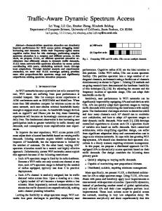
forces behind DSA. However, what is not clear is how the DSA and the presence of secondary market will reshape the radio services market and industry as a whole. The literature lacks a discussion on the potential changes in the market dynamics caused by the possibility of DSA [11]. In this research, we aim to address, the impact of DSA on the dynamics of the primary market. We also propose a different auctioning mechanism in the primary market, that is truthful and more efficient than the simultaneous ascending bid auction currently being used by the FCC [12]. Despite its various virtues, the simultaneous ascending bid auction is not truth revealing and hence not necessarily efficient. The presence of secondary market and the DSA promote speculators’ interest in buying spectrum in the primary market, and trading it for a profit in the secondary market. The colluders find it easier to collude in the primary market and split their winnings in the secondary market in a more socially acceptable way. Studying these effects is computationally challenging because of the difficulty in obtaining the relevant data and the large space of possibilities. The goal of this paper is to develop an efficient computational framework for studying such questions. The paper’s main contributions are summarized below. 1. Agent based tool for wireless spectrum market: Motivated by the computational difficulties of understanding properties and implications of various market clearing mechanisms, we have developed a microscopic agent based simulation tool, S IGMA -S PECTRUM , for trading spectrum in wireless markets. S IGMA -S PECTRUM is a modified version of S IGMA that was originally built to study the restructuring of the electricity market [13], [14]. S IGMA has been customized to S IGMA S PECTRUM to meet the specific needs of the wireless spectrum market. The overall architecture of S IGMA -S PECTRUM is presented in Fig. 1. It is coupled with a detailed synthetic demand model, called S YNTHETIC S PATIO -T EMPORAL R E LATIONAL S ESSION M ODELING E NVIRONMENT (SSRSM), developed in [15] (which also appears in these proceedings), which constructs individualistic demand profiles that vary spatially and temporally. The architecture shows the players in the primary and secondary markets, the market clearing
mechanisms, and the flow of bids, asks and the allocation of licenses. 2. Analysis using SIGMA-SPECTRUM: As an application, we implement an efficient ascending bid auction mechanism by Ausubel [16], which has all the advantages of the ascending bid auction but, in addition, is truthful. It decouples the winners’ bidding price from their payment which results in truth revealing behavior of the bidders. The winner does not pay its bid price; it only pays the opportunity cost of assigning the marginal unit to the winning bidder. 3. Impact of DSA on primary market dynamics: Allowing for potential future trading in a secondary market, we study the impact of various bidding behaviors on the primary market dynamics. Such a resale option can attract speculators to the primary market, and we find that speculators can significantly influence the winning price in the primary market. Also, if a few bidders collude and make their bids jointly, the collusive behavior can be rewarding for all the bidders. Our analysis should be seen as a cautionary note for the regulating authorities and the policy makers. It suggests that changes in the assumptions and bidding behavior can significantly alter the market dynamics in unexpected ways, motivating the need for a detailed agent based tool such as S IGMA -S PECTRUM . The remainder of the paper is organized in the following manner. In section II, we describe the overall architecture of S IGMA -S PECTRUM . In section III, we briefly describe the demand and supply model. Section IV shows the simulation setup, experiments and results. Finally section V provides a brief discussion of the results. II. T HE OVERALL A RCHITECTURE
OF
S IGMA -S PECTRUM
S IGMA -S PECTRUM is a service oriented, high fidelity, computational market modeling tool. Its flexible and modular design allows several regulatory and policy issues to be examined. We first describe the high level architecture, and then discuss the clearing mechanism of Ausubel [16], which is implemented in S IGMA -S PECTRUM . A. The Architecture The overall architecture of S IGMA -S PECTRUM is presented in Fig. 1. It consists of a detailed representation of the synthetic demand model and the market model. It shows how the disaggregated demand profiles are linked to the service providers and the market. It shows the players and the clearing mechanisms in the primary and secondary markets, as well as the flow of bids, asks and allocation of licenses. Individualistic demand profiles built in [15], vary spatially and temporally for each service provider. The demand profiles are mobility and activity based, and include information about the demographics of the population [13]. For instance, the spectrum demand is modeled to be different for a teenager, for a worker, for a retired person etc. based on their specific activities and mobility patterns. The service providers use these demand profiles and a greedy channel allocation scheme to estimate the smallest number of channels or licenses needed
to satisfy the demand. These estimates determine service providers’ bids which go as input to the market model. We find that greedy channel allocation leads to tighter spectrum estimates as compared to the standard reuse factor that accounts for the interference, because of the significant heterogeneity of the demand. The market model is designed to support multiple rounds of bidding and a variety of clearing mechanisms in the primary and secondary market. The market module is coupled with a physical clearing mechanism to resolve physical conflicts pertaining to bandwidth, time, coverage domain etc. that arise in the contracts due to trading in the secondary market [14]. There are a variety of auction mechanisms supported by S IGMA -S PECTRUM . We use Ausubel’s ascending bid auction to allocate the spectrum licenses. B. The Market Clearing Mechanism: Ausubel’s algorithm All bidders designated as “qualified” by the FCC can participate in the auction. Through the licenses, FCC sells the rights to transmit signals over specific bandwidths and geographical regions. The goal of the FCC’s auction is to determine who to allocate the licenses to and at what price. In an ascending bid auction, the price and allocation are determined through an open competition among the bidders. We use an efficient ascending bid auction mechanism [16] to allocate the wireless spectrum licenses by the FCC. This auction mechanism starts with the auctioneer announcing a price and the bidders responding with the number of units they would like to buy. The auctioneer keeps raising the price until the demand is no greater than the supply. At each price, the auctioneer determines if for any bidder i, the aggregate demand of bidder i’s rivals is less than the total supply. If yes, the difference is considered to be “clinched” by the bidder i at the current price. The auctioneer awards the bidder any units clinched at the clinching price and the auction carries on. The auctioneer raises the price again, the bidders adjust their demands given the new price. The auctioneer checks for each bidder if any new units have been clinched. If yes, the auctioneer awards them at the newly clinched price and carries on with the auction by raising the price further. This continues till there is no excess demand. We illustrate this mechanism with an example. Assume there are 6 licenses to be distributed between 4 service providers A through D whose valuations are as given in Table II. The bidding starts at $1m. Given the valuations, A and B demand 3 units and C and D demand 2 units each. The total demand exceeds the total supply so the price continues to rise. As price rises to $3m, B reduces its demand to 2 units and C reduces its demand to 1 unit because B values the third unit at $3m at which he makes no profit from the third unit and similarly, C makes zero profits from the second unit at $3m. The overall demand in the market is still greater than the total supply of 6. Now, if one looks at the sum of demand of A’s rivals, it is only 5 units whereas the supply is 6. This means A is guaranteed to win the first license if everyone continues
to bid based on their downward sloping demand curves. A clinches the first license at $3m. Now the price rises to $3.5m. At this price, A demands 3 units, B demands 2 units and C and D demand 1 unit each. Again, A’s rivals together are only demanding 4 units, which means A is guaranteed to win the second unit as well. This he wins at price $3.5m. Now look from B’s perspective. All of B’s rivals together are demanding only 5 units whereas the supply is 6 so he clinches the 3rd unit, also at $3.5m. If C or D drop out, there is no excess supply so none of them clinches any license at $3.5m. If one looks at the overall market there is still excess demand. So the price continues to rise. At $4m, A demands 2 units, B demands 2 units and C and D demand 1 unit each. Now there is no excess demand. Supply equals demand and the auction comes to an end. The final allocation gives A and B two licenses each and C and D one license each. A gets the first at a price of $3m, second at $3.5m, B gets the first at $3.5m, second at $4m and C and D get their licenses at $4m each. This auctioning mechanism has many advantages over the method currently used by FCC. •
•
•
•
•
•
This auction mechanism motivates the bidders to bid truthfully. It is structured such that the winner’s price is independent of his own bids. It depends solely on his competitors’ bids. This incentivizes each bidder to truthfully reveal his valuation for the licenses [17]. The allocation is efficient since licenses are clinched by the bidders who value them the most. This auction operates in an open and transparent manner. Maximum information is made available to each participant at the time the bidding is placed. Value is socially determined through the increased bids. The bidders learn from each others’ bidding and continuously adjust their valuations. Open bidding competition and transparency of information prompt bidders to bid more aggressively. They get an opportunity to revise their value estimates after each bidding round. This raises their confidence in bidding and reduces winner’s curse. Given the fact that the licenses can possibly be resold in the secondary market, this value revealing process is all the more important. It preserves the privacy of the bidders. The winning bidders do not have to reveal their entire demand curves. They only reveal the portion of the demand curve that is below the winning price. Ascending bid auction shares some of the virtues with the Vickrey auction, but has clear advantages over the Vickrey auction. Unlike Vickrey, ascending bid is easier to implement, does not leave any money on the table, and does not leave room for corruption. For example, under the sealed bid Vickrey auction, corruption can occur because the seller has an incentive to submit a fake bid for just under the amount of the highest bid [18]. Experimental evidence shows that ascending bid auctions are more efficient than the sealed bid Vickrey auction because the incentive for playing the efficient dominant
strategy is clearer to bidders [19]. III. D EMAND
AND
S UPPLY
A key feature of the architecture is the accurate modeling of individualistic demand that varies spatially and temporally. Service providers’ demand bids are based on this demand. Generation of demand profiles and their assignment to service providers is a crucial step for the study described here and is based on a synthetic wireless network traffic model [15]; we describe it briefly in Section III-A. Section III-B describes how it is used to construct inputs required for the market model. A. Network traffic modeling Real data for wireless cellular traffic is very difficult to access because of proprietary reasons. For the study described here, we use the models from [15] to generate the demand for wireless spectrum at detailed spatio-temporal scale for the city of Portland, Oregon. It combines a variety of different data sets and models as shown in Fig. 1, including: an urban mobility model, [20], synthetic social network of Portland [20], [21], road network data, data sets for device ownership from NHIS [22], and aggregate characteristics for cellular communication traffic, such as call arrival rate and call duration [23], [24]. To characterize the spatio-temporal demand variation in the city of Portland, the city is divided into 2109 cells, denoting the coverage areas for each cell tower. The wireless traffic is generated by synthetic individuals with demographic attributes that statistically match the real population of Portland [20]. The mobility of the synthetic individuals occurs on the Portland road network and is determined by an activity-based mobility model. For instance, if an individual moves from location l1 in cell C1 to l2 in C2 , then the mobility model tracks him/her along the road network connecting l1 and l2 . Thus, the contribution of the user to each cell’s load is collected in a more accurate way. The demand model generates wireless calls (or call sessions) for each individual from the synthetic population for the duration of a day using statistics in [23]. By integrating the cells, mobility of individuals and the call sessions, we generate the call volumes for every service provider’s cell tower in the city. This call volume is translated into required channels and licenses in each cell (details of this conversion is provided below). This spectrum demand is used to drive the market strategies employed by the individual service providers to obtain spectrum from FCC. We first describe the notations used here. A call from a person u to another person v starting at time t1 and terminating at t2 is denoted by a tuple (u, v, [t1 , t2 ]). For a cell C and time interval T , A(C, T ) defines the set of calls from or to a person who is located within C and is in a session with a time overlap in the interval T . We define load L(C, T ) as: L(C, T ) = max h(C, t′ ), ′ t ∈T
(1)
where h(C, t′ ) is the number of calls in A(C, T ) that are simultaneously active at time t′ —this captures the peak number of simultaneous calls in C during the time interval T . T defines the periodicity with which the load is determined
Market Mechanisms
SSRSM Synthetic Population
Suppliers Primary Market
Activity Data Bids Device Ownership (NHIS Data)
MARKET MODEL
Vickrey Ascending Bid Auction
Individual Demand Profiles
Channel Allocation
Service Providers
Multiple Rounds
Speculators
Portland Road Network Data
Bids and Asks Secondary Market
FCC Primary Allocation
Secondary Allocation Economic Contracts
Resolve Physical Conflict
Bilateral
Market Clearing Mechanisms Centralized
Clearing
Fig. 1: Elements of the overall architecture of S IGMA -S PECTRUM . SSRSM refers to the synthetic demand model developed in [15].
0: 00
6: 00
S−−N
100 S−−N
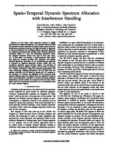
and the granularity with which the market mechanisms are designed. For the purposes of this paper, we assume T = 1 hr and can be changed in accordance to the minimum intervals at which the market mechanisms are triggered. We calculate the hourly peak load, i.e., L(C, T ) during a given hour T , in each cell C of the city; contour maps illustrating the load at few representative hours are shown in Fig. 2.
90 80
W−−E
W−−E
9: 00
12: 00
70
S−−N
50 40
W−−E
W−−E
17: 00
22: 00
30
S−−N
20 S−−N
Constructing bid functions require determining the spectrum resources needed to support the call volume in the model, and then translating it into the number of channels and licenses. For simplicity, we assume GSM is the underlying cellular technology although a similar process can be done for a CDMA or any other system. The parameters used below are representative of GSM technology (based on available literature) but the calculations can be done for any other system parameters, without loss of generality. In North America, the total bandwidth for both an uplink and a downlink in GSM communication is commonly 25 MHz. Each band is subdivided into 124 carrier frequencies spaced 200 kHz apart using frequency division multiple access (FDMA) techniques and further sub-divided into 8 time slots using time division multiple access (TDMA), such that each channel consists of 8 slots that can accommodate up to 8 cellular users simultaneously. When a mobile device initiates a call or receive a call, a two-way voice communication session is established between the device and its base station and a circuit connection is set up between the two base stations. The communication between a device and a base station requires one channel (called the forward channel) for the uplink and one channel
S−−N
60
B. Constructing Bid Functions
W−−E
10
W−−E
Fig. 2: Spatial view of peak load in the Portland area at midnight, 6AM, 9AM, 12 Noon, 5PM and 10PM.
for the downlink, (called the reverse channel) from the base station to the cell phone. Therefore, for each cell and for each provider, we can calculate the number of channels required to support the peak load. We assume that interference would occur if two active devices within a cell or in neighboring cells use the same channel. To avoid interference, the neighboring cells have to
be assigned distinct channels. A reuse factor (typically 4) is commonly used to account for this interference. Based on this factor, the number of channels needed can be bounded by 4 times the number of channels needed in the most heavily loaded cell. However, using the heterogeneous space-time load profile (from Section III-A), we can get a better estimate of the reuse by means of a greedy channel allocation algorithm described in Algorithm 1 below. Our simulation results show that the Greedy Channel Allocation method provides more economic bandwidth demand estimates for the service providers. These estimates require about 50% less channels or licenses to serve the demand as compared to the estimates from the reuse factor scheme. Greedy Channel Allocation. For a load function L(C, [t1 , t2 ]) that specifies the number of channels needed for cell C during the time interval [t1 , t2 ], we use a greedy channel allocation scheme to estimate the smallest number of channels needed to satisfy the load. Let S = {c1 , c2 , ..., cn } denote the set of available channels, WC the set of channels that are assigned to cell C, and let the number of cells be B. We sequence the cells horizontally, i.e., numbering a cell at row x and column y by (x − 1) × COL+ y where COL is the number of columns in the rectangle area. Our algorithm considers cells in this sequence, which turns out to be crucial. S Algorithm 1 Greedy-Coloring( C {L(C, [t1 , t2 ])}): Greedy coloring algorithm for assigning channels to cells 1: for i = 1 to B do 2: Wi = ∅ 3: end for 4: for i = 1 to B do S 5: W = j Wj , where j < i and cell j is adjacent to cell i. 6: Let Wi be the lowest numbered L(i, [t1 , t2 ]) channels in S that do not lie in W 7: end for After running the algorithm, the number of required channels N ([t1 , t2 ]) during [t1 , t2 ] can be determined by [ N ([t1 , t2 ]) = | Wj | j
The license demand D([t1 , t2 ]) during this time interval [t1 , t2 ] can be calculated by D([t1 , t2 ]) = N ([t1 , t2 ])/NL
(2)
C. Supply We assume that the FCC is the only supplier in the primary market. It has a fixed number of licenses that it wants to auction off. We assume that there is no cost to FCC in obtaining and auctioning the wireless spectrum. So all revenue generated is equal to FCC’s profit. The supply curve of FCC looks like a vertical line since it is willing to sell a fixed number of licenses at the highest possible price.
IV. T HE S IMULATION S ETUP We simulate a primary market in which the seller, FCC, is offering to sell 10 licenses of the wireless spectrum. These licenses give the bidders a right to utilize certain frequencies over the city of Portland. We assume that all licenses have the same features in terms of their bandwidth, power levels, coverage area etc. The experimental settings are outlined in Fig. 3. The market shares in Fig. 3 are assigned to simulate realistic representation of market shares of the service providers Verizon, ATT, Sprint-Nextel, T-mobile etc. The synthetic demand module ensures that the load generated for each service provider approximately matches its market share. • • • •
• • • •
Location: Portland, Oregon Number of Originally Available Licenses: 10 Service Providers: A, B, C, D, E, F Market Share of providers: 29%, 30%, 18%, 12%, 6% and 5% Speculators: G & H Minimum Bid Price: $1 million Reservation Price: $350k Capacity of Each License: Table II through Table XV - Each license serves 10% of the market Table XVI through Table XIX - Each license serves 5% of the market. Fig. 3: Experimental settings for the market study.
In the first set of experiments, we assume that each license has enough capacity to serve about 10% of the Portland demand. Based on this, each service provider estimates the number of licenses required to serve its customers in the retail market. However, some bidders may demand more than what is needed because they anticipate reselling it at a higher price in the secondary market, whereas others may demand less than what is needed if they are concerned about the prices falling in the secondary market. Historical evidence shows that postauction prices can be below auction prices as was the case for the wine auctions in France [25]. We also assume that there are two speculators present in this market. The speculators do not service any customers. Their only goal is to earn money through arbitrage by buying low in the primary market and selling high in the secondary market. In this paper, we focus on understanding the dynamics of the primary market based on the above setup. The secondary market will be described in detail in a follow-up paper. In order to be a qualified bidder, we assume that the FCC requires the bidders to deposit an upfront payment of $350k per license for the maximum number of license that they expect to bid. For example, if a bidder expects to bid for 2 licenses at the most, he has to deposit $700k. This reservation price is to ensure sincere bidding. Any withdrawal penalties are taken from the bidder’s upfront payment.
Table Table Table Table
II III IV V
Table Table Table Table Table Table Table Table
VI VII VIII IX X XI XII XIII
Table XIV Table XV Table Table Table Table
XVI XVII XVIII XIX
Base Case Original valuations. Base0, allocations when only service providers bid. Base1, allocations with service providers plus one speculator. Base2, allocations with service providers plus two speculators. Variation in Demand Valuations under reduced demand. Allocations under reduced demand. Valuations under increased demand. Allocations under increased demand. Valuations under 50% increase, 50% decrease but no net change in demand. Allocations, 50% increase, 50% decrease, no net change in demand. Valuations under random change in demand. Allocations, random change in demand. Collusive Behavior Allocations, collusion among service providers, valuations as in Table II. Allocations, collusion among speculators, valuations as in Table II. Reduced License Capacity Valuations under reduced license capacity of 5%. Allocations, reduced license capacity, only service providers bid. Allocations, reduced license capacity, service providers and one speculator bid. Allocations, reduced license capacity, service providers and both speculators bid. TABLE I: Summary of experiments and the tables.
A. The Valuation Model We assume a common value model for the demand estimates. In the common value model, the licenses are worth the same to everyone but each bidder makes an independent estimate of this uncertain value. There are many reasons why common value uncertainties arise among bidders [26]. They are largely because each bidder has a personal estimate of (i) what the license will be worth in the retail market, (ii) what its value will be in the secondary market where the service providers trade among each other to overcome their surplus and deficits, (iii) when might FCC announce the auction of more licenses in future, (iv) what might be the impact of technological improvements on the current set of licenses, and (v) what market share can be sustained and how fast will the market grow in demand for such services. We assume that the bidders derive their values from {1, 1.5, 2, 2.5, . . . , 9, 9.5, 10} uniformly at random. These common value uncertainties affect the value estimates of the bidders and hence their bids. The difference in the value estimates conveys negative information, about winning, to some extent. This is because winning implies that the winner overestimated the value of the license the most, also known as winner’s curse. However in the ascending bid auction, this curse is mitigated because in each round the bidders have an opportunity to adjust their value estimates based on the new information [26] announced by the competitors. In addition, the winner only pays the opportunity cost of the license which is always lower than what he values the license at.
Value unit 1 unit 2 unit 3
A 5.5 5 4
B 7.5 6 3
C 7 3 0
D 4.5 3.5 0
E 5 0 0
F 3.5 0 0
G 6.5 5 0
H 7.5 6 0
TABLE II: Bidders’ Valuations in Millions of Dollars.
B. Base Case With and Without Speculators In this section, we evaluate the market with (1) only service providers and no speculators and (2) both service providers and speculators. We are assuming the bidders’ marginal valuations for the licenses are as given in Table II. We also assume that the licenses are identical in characteristics and the minimum bid price is set at $1 million. In the base case, we consider only the service providers, A, B, C, D, E, and F to be the bidders. Later, the speculators G and H join as bidders. We refer to the study with one and two speculators as base1 and base2, respectively. First, we consider the case with no speculators. The efficient ascending bid auction mechanism [16] allocates the licenses to the winning bidders at the winning prices as specified in Table III. In the base case, only the six service providers submit the bids and each demands the minimum number of licenses needed to serve the demand in the retail market. Now, assume that FCC allows dynamic spectrum access which implies that any licenses bought in the primary market can be resold in a secondary market. The possibility of a secondary market where spectrum is resold, invites speculators to the primary market. We expect the presence of speculators will
License ID Winners Win Price License ID Winners Win Price
1 A 1 7 D 3
2 B 1 8 D 3
3 A 3 9 E 3
4 A 3 10 F 3
5 B 3
Value unit 1 unit 2 unit 3
6 C 3
1 A 3 7 D 3.5
2 A 3.5 8 E 3.5
3 A 3. 5 9 G 3.5
4 B 3.5 10 G 3.5
5 B 3.5
6 C 3.5
raise the winning price and the allocations. We first include one speculator only and observe the effect on the winning price. Assume speculator G joins the 6 service providers in bidding. This changes the license allocations and winning prices to what is shown in Table IV. The addition of one speculator raises the winning price for all the licenses, and the speculator G wins two of the licenses that had previously gone to the service providers. Next, assume both G and H join the bidding in this market. The bids are based on their valuations specified in Table II. Their entry into the market changes the winning bidders and winning prices as specified in Table V. Observations: The addition of speculators to the market raises the prices on all licenses. When G entered the market, service provider D and F lost one license each to G. The winning price of all the licenses is higher than the base case of no speculators. When speculator H entered the market, the prices went up even higher and 4 out of 10 licenses were won by the speculators. FCC’s revenue increased from $26 million in base case to $42.5 million in the presence of speculators.
1 A 3.5 7 C 4.5
2 B 4 8 E 4.5
3 G 4 9 G 4.5
4 H 4 10 H 4.5
C 7 3 0
D 4.5 0 0
E 0 0 0
F 0 0 0
G 6.5 5 0
H 7.5 6 0
License ID Winners Win Price License ID Winners Win Price
1 B 1 7 G 3
2 A 3 8 G 3
3 A 3 9 H 3
4 B 3 10 H 3
5 C 3
6 D 3
TABLE VII: License allocations under reduced demand
C. Demand Manipulation
TABLE IV: License allocations in the presence of one speculator and six service providers.
License ID Winners Win Price License ID Winners Win Price
B 7.5 6 3
TABLE VI: Bidders’ new valuations when the demand is reduced compared to base2.
TABLE III: License allocations for the base case: Only the six service providers participate in the auction. No speculators are present.
License ID Winners Win Price License ID Winners Win Price
A 5.5 5 0
5 A 4.5
6 B 4.5
TABLE V: License allocations for base2: Two speculators join the six service providers.
The possibility of buying and selling the deficit or excess spectrum in the secondary market affects the dynamics of the primary market. In addition to attracting speculators, service providers may now alter (inflate or deflate) their true demand with the expectation that spectrum sale in secondary market may fetch higher returns. In this section, we evaluate the effect of this behavior on the dynamics of the primary market and the winning price. We perform 4 sets of experiments. In the first one, we assume that some of the service providers demand less than what they need, in the second one, some demand more than what they need, in the third one, half of them demand more and the other half demand less so that there is no net change in demand and in the fourth one, the service providers make random changes where they increase, decrease or keep their demand the same. Reduction in Demand: Some service providers may believe that reducing demand in the primary market will reduce the price for everyone. So, they decide to demand only a fraction of the spectrum needed to serve their customers in the retail market. They may also reduce the demand if they expect that prices in the secondary market will be lower than the primary market. Table VI shows the effect on their valuations due to this strategy. The experiment evaluates the effect of such a strategy on the market and the price of the spectrum. The results are shown in Table VII. This clearly results in much lower prices for all the licenses compared to base1 and base2. All bidders gain from the demand reduction behavior. The overall cost of the licenses in this scenario is reduced to $28m as compared to $34.5m in base1 and $42.5m in base2. Inflated Demand: Some service providers may believe that the resale of spectrum in the secondary market will be profitable and so they demand extra in the primary market. The new valuations for this inflated demand are shown in Table VIII. When the revised demand estimates are used in the auction, the allocations change to the set of winners and winning prices
Value unit 1 unit 2 unit 3 unit 4
A 5.5 5 4 3.5
B 7.5 6 3 0
C 7 3 2.5 0
D 4.5 3.5 0 0
E 5 4.5 0 0
F 3.5 3 0 0
G 6.5 5 0 0
H 7.5 6 0 0
TABLE VIII: Bidders’ new valuations when the demand is increased compared to base2.
License ID Winners Win Price License ID Winners Win Price
1 A 4.5 7 G 4.5
2 A 4.5 8 G 4.5
3 B 4.5 9 H 4.5
4 B 4.5 10 H 4.5
5 C 4.5
6 E 4.5
TABLE IX: License allocations with expanded demand
License ID Winners Win Price License ID Winners Win Price
1 A 4.5 7 G 4.5
2 A 4.5 8 G 4.5
3 B 4.5 9 H 4.5
4 B 4.5 10 H 4.5
5 C 4.5
6 E 4.5
TABLE XI: License allocations when some providers increase and others reduce their demand such that the total demand remains unchanged. Value unit 1 unit 2 unit 3 unit 4
A 5.5 5 4 3.5
B 7.5 6 0 0
C 7 3 2.5 0
D 4.5 0 0 0
E 5 0 0 0
F 3.5 0 0 0
G 6.5 5 0 0
H 7.5 6 0
TABLE XII: Bidders’ new valuations when service providers randomly change their demand. as displayed in Table IX. The total cost of the licenses now increases to $45m, higher than the base2 where the total cost was $42.5m. Experiments shown in Table VII and IX provide further evidence to the results that the overall demand reduction reduces the total revenue and demand inflation increases the total revenue. Mixture of Demand Reduction and Expansion: Next, we consider a scenario where some bidders demand less than what they need and others demand more than what they need. In this experiment, we assume that 50% of the service providers reduce their demand while 50% of the service providers increase their demand. Again, the speculators do not change their bids. The resulting valuations are displayed in Table X. These new valuations result in allocations shown in Table XI. In this case, the total cost of the licenses is again $45m. This number could have been higher or lower depending upon which service providers raised and lowered their bids. Now, we let service providers randomly decide whether to reduce the demand, increase the demand or keep it the same. We assume that the speculators do not change their bids. All bidders’ revised valuations appear in Table XII and the allocations in Table XIII. In this case, the total cost of licenses is the same as was in case 2, i.e. at $42.5m. Observations: The above set of experiments show how the dynamics in the primary market are impacted when the possiValue unit 1 unit 2 unit 3
A 5.5 5 4
B 7.5 6 0
C 7 3 2.5
D 4.5 0 0
E 5 4.5 0
F 3.5 3 0
G 6.5 5 0
H 7.5 6 0
TABLE X: Bidders’ new valuations when 50% service providers increase their demand and 50% reduce their demand. The total demand remains unchanged.
bility of DSA is present. The expectation of service providers regarding the secondary market and the presence of speculators can significantly change the bidding behavior of all the bidders in the market. Even when a truthful mechanism is in place, the uncertainties about the secondary market can greatly influence the bidding strategies of the market players. D. Collusive Behavior One of the ways to manipulate auction outcomes is through engaging in collusive behavior. Collusive behavior can reduce the winning price of not only the colluders but other winners as well. This is true even when there is no change in the number of licenses demanded or the valuations of the bidders. For example, if service provider B colludes with service provider E and they together bid for 4 licenses at the same valuations, the winning allocations appear as specified in Table XIV. This allocation when compared with base2 shows that B and E together paid $1m less for the three licenses under collusion. Before B paid $4m for the first one and $4.5m for the second and E paid $4.5m for his first one. Now they paid $3.5m, $4m and $4.5m respectively for the three license that B obtained; two for himself and one for E. Now, if both speculators G and H decide to collude with
License ID Winners Win Price License ID Winners Win Price
1 A 3.5 7 C 4.5
2 B 4 8 E 4.5
3 G 4 9 G 4.5
4 H 4 10 H 4.5
5 A 4.5
6 B 4.5
TABLE XIII: License allocations under random change of demand by service providers.
License ID Winners Win Price License ID Winners Win Price
1 A 3.5 7 B 4.5
2 B 3.5 8 C 4.5
3 B 4 9 G 4.5
4 G 4 10 H 4.5
5 H 4
6 A 4.5
TABLE XIV: License allocations under collusive behavior. Bidder B colludes with bidder E. License ID Winners Win Price License ID Winners Win Price
1 A 3.5 7 B 4.5
2 G 3.5 8 C 4.5
3 G 3.5 9 E 4.5
4 B 4 10 G 4.5
5 G 4
6 A 4.5
TABLE XV: License allocations under collusive behavior. Speculators G and H collude with each other.
each other and bid for 4 licenses at the same valuation, the allocations will change to the ones specified in Table XV. This shows that they are able to save $1.5m on the four licenses as compared to the base2 case. E. Reduced Capacity of Licenses In earlier set of experiments, we assumed that each license serves 10% of the Portland market. In this section, we evaluate the effect of license capacity on the market dynamics. In particular, we study how the market dynamics change when the license is made up of a smaller number of channels. We reduce the license capacity to half so that each license now serves 5% of the market share. However, there are twice as many licenses available. The question we are trying to answer from this study is if the FCC created smaller units to license how will the bidding process and market efficiency be affected? The number of licenses available for sale is now 20 so as to keep the sum of capacity of all the licenses to be the same. The bidders adjust their demand based on their market share and the new capacity of the licenses. Given that the capacity of the licenses have dropped to half, the bidders drop their valuations to half for each unit. If a bidder was demanding one unit at $5m before, he will demand two units at $2.5m each now. In case of service providers D and F, who need to serve the market share of 12% and 5% respectively, the demand drops to 3 and 1 license respectively. Previously, D needed 2 and F needed 1 license, with 10% market capacity each, to serve its market share. Now the demand of 3 and 1 license is enough with each license serving 5% of the market capacity. Table XVI displays the new marginal valuations of the bidders. Table XVII provides the new allocations when only bidders A through F are bidding and there are no speculators present. The total revenue generated for FCC from these
Value unit 1 unit 2 unit 3 unit 4 unit 5 unit 6
A 2.75 2.75 2.5 2.5 2 2
B 3.75 3.75 3 3 1.5 1.5
C 3.5 3.5 1.5 1.5 0 0
D 2.25 2.25 1.75 0 0 0
E 2.5 2.5 0 0 0 0
F 1.75 0 0 0 0 0
G 3.25 3.25 2.5 2.5 0 0
H 3.75 3.75 3 3 0 0
TABLE XVI: New valuations given the reduced capacity of licenses.
License ID Winners Win Price License ID Winners Win Price License ID Winners Win Price
1 A 0.5 8 B 0.5 15 D 1.5
2 A 0.5 9 C 0.5 16 E 1.5
3 A 0.5 10 C 0.5 17 E 1.5
4 A 0.5 11 D 0.5 18 F 1.5
5 B 0.5 12 A 1.5 19 B 3.5
6 B 0.5 13 A 1.5 20 B 3.5
7 B 0.5 14 D 1.5
TABLE XVII: License allocations under reduced license capacity, only service providers bid, no speculators present.
allocations is $23m which is $3m lower than the case when the licenses had the capacity of serving 10% of the market. Observations: The finer split of the license capacity makes it a more efficient market for the bidders who can reduce their demand to match it more exactly to their needs. Table XVIII shows the license allocation results when the speculator G joins the market and Table XIX displays it for the case when both speculators, G and H, join the market. In both cases, the FCC makes more revenue compared to the no-speculator case. However, in both cases, the FCC makes less or equal amount of revenue than it did before when the licenses had more capacity.
License ID Winners Win Price License ID Winners Win Price License ID Winners Win Price
1 A 1.5 8 G 1.5 15 C 1.75
2 A 1.5 9 G 1.5 16 D 1.75
3 A 1.5 10 A 1.75 17 E 1.75
4 A 1.5 11 A 1.75 18 E 1.75
5 B 1.5 12 B 1.75 19 G 1.75
6 B 1.5 13 B 1.75 20 G 1.75
7 D 1.5 14 C 1.75
TABLE XVIII: License allocations under reduced license capacity, one speculator added
1 A 1.75 8 H 2 15 E 2.25
2 A 1.75 9 A 2.25 16 E 2.25
3 B 2 10 A 2.25 17 G 2.25
4 B 2 11 B 2.25 18 G 2.25
5 G 2 12 B 2.25 19 H 2.25
6 G 2 13 C 2.25 20 H 2.25
7 H 2 14 C 2.25
TABLE XIX: License allocations under reduced license capacity, two speculators added
1
0.8
0.6 Excess Ratio
License ID Winners Win Price License ID Winners Win Price License ID Winners Win Price
0.4
0.2 A B C D E F
0
−0.2
−0.4
0
5
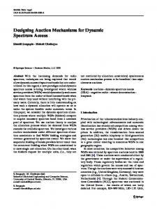
In this section, we compare the efficiency of various allocation outcomes. Due to the page limit, only a select few representative experiments are shown to illustrate the findings. We define a metric, called excess ratio, to measure the efficiency. Let S denote the set of available channels from the allocated licenses, and R(t) denote the set of channels required to satisfy the load at time t. Then, excess ratio at time t, denoted as δ(t), can be expressed by δ(t) = (|S| − |R(t)|)/|S|. A positive value of δ(t) means a surplus while a negative value means a deficiency. A value close to zero represents most efficient usage. In the original base case experiment, we assume each license has a bandwidth of 4.5 MHz. According to the results from the synthetic demand model, service providers have the following bandwidth demands and the corresponding license demands: A - 12 MHz (3 licenses), B - 12.42 MHz (3 licenses), C - 7.45 MHz (2 licenses), D - 4.97 MHz (2 licenses), E - 2.49 MHz (1 license), F - 2.07 MHz (1 license). The license allocation is shown in Table III. Fig. 4 shows the excess ratios of base case 0 at different hours during the entire day; each line represents a service provider, A through F. The figure shows that the excess ratio for all service providers drops significantly during peak hours from 10AM to 7PM (Hour 0 corresponds to midnight). From midnight to the early morning hours and then again after around 8pm, the surplus of channels is high for all the service providers. Across different service providers, it is easy to see that the service providers who got more bandwidth through allocated licenses than needed to satisfy their demand have higher excess ratios. Other service providers, such as B and C, obtain less licenses than what they demanded in the auction. As a result, their excess ratios have negative values during the peak hours. Fig. 5 illustrates the excess ratio of service provider D for three experiments, i.e., base case 0 without speculators (Table III), base case 1 with one speculator (Table IV) and reduced license capacity case without speculators (Table XVII). Entry of speculator in the market reduces the excess ratio of D because the speculator wins the license that was allocated to D in base case 0. Moreover, the experiment with reduced
10
15
20
25
Hour
F. Efficiency of License Allocation
Fig. 4: Excess ratios of all service providers during a 24 hour period.
license capacity shows a lower positive excess ratio, i.e., higher efficiency, than base case 0. This validates our hypothesis that the finer split of the license capacity makes it a more efficient market for the bidders who can reduce their demand to match it more exactly to their needs. Fig. 6 illustrates the spatial and temporal view of excess channels, for service provider A, for base case with two speculators in the Portland area. For cell i, the number of excess channels can be determined by |Si | − |Ri (t)|, where Si is the set of channels allocated to cell i and Ri (t) is the set of channels needed to meet the load. Again, a positive value means a surplus of channels while a negative value means a deficit. Results show that day time hours have less surplus channels than night time hours. Also, the downtown area, located in the middle of the map, has high usage of channels compared to the rest of Portland. In the day time, in the downtown area, most of the channels stay active and have very little surplus. However, in the night time, the surplus number of channels can be as high as 80. In downtown, there is occasional channel deficiency but in other areas, there are sufficient number of channels to meet the load. G. Summary of Results We develop a computational framework for studying some of the emerging issues in the spectrum markets. It is coupled with a detailed disaggregated demand model and a physical clearing module. A truthful, ascending bid, auction mechanism is implemented to allocate licenses in the primary market. The following broad conclusions are derived from the simulation experiments: • When speculators join the market, the prices go up on all the units. This result holds even when the bids submitted by the speculators are low and none of the licenses are actually won by the speculators.
1.2 Base Case 0 Base Case 1 − One Speculator Reduced License Capacity
1
0.8
6: 00
S−−N
S−−N
0: 00
80
W−−E
W−−E
9: 00
12: 00
60
0.6
20
0.4
−0.2
0
5
10
15
20
Fig. 5: Excess ratios of service provider D for three different experiments: base case, base case with one speculator, and reduced license capacity.
•
•
22: 00
0
−20
25
Hour
•
W−−E
17: 00
S−−N
0
W−−E
S−−N
0.2
•
S−−N
S−−N
Excess Ratio
40
The possibility of the secondary market can change the valuations of the bidders in the primary market as their projections about the prices in the secondary market change. This may prompt them to demand more or less than their true needs. As a result, if the market faces overall reduced demand, the winning prices drop on all the licenses. In case of excess demand, the opposite occurs. Table XI shows that even though the overall demand and valuations are unchanged in the market, a different split of the valuations among the bidders can change the winning prices substantially. Table XIV and XV show that when service providers B and E collude and when speculators G and H collude, they benefit significantly from this collusive behavior. Our experiments also show that depending upon the marginal valuations, the collusive behavior can be rewarding to not just the colluders but also other winners. The results show that when the FCC splits the licenses into finer chunks, the bidders can match their demand more exactly to their needs which in turn reduces the revenue for FCC but results in lower prices for the bidders. The results show the spatial and temporal distribution of the demand and supply in the Portland area. The efficiency of channel usage is highest in the downtown area and during the peak hours from 10AM to 7PM.
W−−E
W−−E
Fig. 6: Spatial view of excess channels of service provider A for the base case 2 in the Portland area at midnight, 6AM, 9AM, Noon, 5PM and 10PM.
V. D ISCUSSION The new policy trend of making the spectrum access dynamic in the spatial and temporal dimensions is intended to reduce inefficiencies in spectrum utilization that are caused by its static partitioning. This research takes a step in identifying some of the issue that are likely to arise from this new trend. The paper shows that the possibility of trading in the secondary market has significant repercussions on the bidding behavior of the service providers in the primary market as well. For example, the service providers can now buy more or less spectrum than what is truly needed to serve their customers. This can change their marginal valuations, bidding strategies and hence auction outcomes. Speculators can join the market and make profits through arbitrage. The possibility of collusive behavior is increased since bidders who needed only a fraction of the license (for instance, E and F only needed half a license each to serve the demand in the retail market when each license could serve up to 10% of the market share) can now collude and split the capacity later. Usually this kind of weakness is overcome by structuring licenses, in terms of their geographical scope and the band plan, in such a way that splitting up the spectrum becomes difficult for the bidders in the secondary market. Acknowledgements: We thank our external collaborators and members of the Network Dynamics and Simulation Science Laboratory (NDSSL) for their suggestions and comments. This work has been partially supported NSF Nets Grant CNS-0626964, NSF HSD Grant SES-0729441, NSF PetaApps
Grant OCI-0904844, DTRA R&D GrantHDTRA1-0901-0017, DTRA CNIMS Grant HDTRA1-07-C-0113, NSF CAREER CNS 0845700 and NSF NETS CNS-0831633. R EFERENCES [1] M. Scanlan, “Hiccups in us spectrum auctions,” Telecommunications Policy, vol. 25, no. 10-11, pp. 689–701, 2001. [2] I. O. and N. Mandayam, “Dynamic Spectrum Access Models: Toward an Engineering Perspective in the Spectrum Debate,” IEEE Communications Magazine, January 2008. [3] Peha J. M., “Approaches to Spectrum Sharing,” IEEE Communications Magazine, February 2005. [4] Doerr C., Grunwald D. and D. Sicker , “Local Control of Cognitive Radio Networks,” Ann. Telecommun., March 2009. [5] H. Mutlu, M. Alanyali, and D. Starobinski, “On-line pricing of secondary spectrum access with unknown demand function and call length distribution,” in INFOCOM 2010, IEEE, San Diego, USA, March 2010. [6] A. A. Daoud, M. Alanyali, and D. Starobinski, “Pricing strategies for spectrum lease in secondary markets,” Networking, IEEE/ACM Transactions on, in press. [7] H. Mutlu, M. Alanyali, and D. Starobinski, “Spot pricing of secondary spectrum usage in wireless cellular networks,” in INFOCOM 2008, IEEE, April 2008, pp. 682– 690. [8] M. M. Buddhikot, “Understanding dynamic spectrum access: Models, taxonomy and challenges,” in Proceedings of IEEE DySPAN07, Dublin, Ireland, April 2007. [9] M. M. Buddhikot and K. Ryan, “Spectrum management in coordinated dynamic spectrum access based cellular networks,” in Proceedings of IEEE DySPAN05, Baltimore,Maryland, November 2005. [10] A. P. Subramanian, H. Gupta, S. R. Das, and M. M. Buddhikot, “Fast Spectrum Allocation in Coordinated Dynamic Spectrum Access Based Cellular Networks,” in Second IEEE International Symposium on New Directions in Dynamic Spectrum Access Networks (DySPAN 2007), Dublin, Ireland, April 2007. [11] Chapin J.M. and W.H. Lehr, “The Path to Market Success for Dynamic Spectrum Access Technology,” IEEE Communications Magazine, May 2007. [12] P. Milgrom, “Putting auction theory to work: The simultaneous ascending auction,” Journal of Political Economy, vol. 108, pp. 245–272, 2000. [13] K. Atkins, A. Marathe, and C. Barrett, “A computational approach to modeling commodity markets,” Computational Economics, vol. 30, no. 2, pp. 125–142, September 2007. [14] K. Atkins, J. Chen, A. Kumar, M. Macauley, and A. Marathe, “Locational market power in network constrained markets,” Journal of Economic Behavior and Organization, vol. 70, no. 1-2, pp. 416–430, May 2009. [15] R. Beckman, K. Channakeshava, F. Huang, V. A. Kumar,
[16]
[17]
[18]
[19]
[20]
[21]
[22]
[23]
[24]
[25]
[26]
A. Marathe, M. Marathe, and G. Pei, “Synthesis and analysis of spatio-temporal spectrum demand patterns: A first principles approach,” IEEE Dynamic Spectrum Access Networks, DySPAN, April 2010. L. M. Ausubel, “An efficient ascending-bid auction for multiple objects,” American Economic Review, vol. 94, no. 5, pp. 1452–1475, December 2004. W. Vickrey, “Counterspeculation, auctions, and competitive sealed tenders,” The Journal of Finance, vol. 16, no. 1, pp. 8–37, 1961. M. H. Rothkopf, T. J. Teisberg, and E. P. Kahn, “Why are vickrey auctions rare?” Journal of Political Economy, vol. 98, no. 1, pp. 94–109, February 1990. J. H. Kagel, R. M. Harstad, and D. Levin, “Information impact and allocation rules in auctions with affiliated private values: A laboratory study,” Econometrica, vol. 55, no. 6, pp. 1275–1304, November 1987. C. Barrett, D. Beckman, M. Khan, V. A. Kumar, M. Marathe, P. Stretz, T. Dutta, and B. Lewis, “Generation and analysis of large synthetic social contact networks,” in Winter Simulation Conference, 2009. Network Dynamics and Simulation Science Lab, Virginia Tech, “Synthetic data products for societal infrastructures and proto-populations,” ndssl.vbi.vt.edu/opendata. Center for Disease Control, “National health interview survey (nhis),” http://www.cdc.gov/nchs/about/ major/nhis/nhis 2007 data release.htm. D. Willkomm, S. Machiraju, J. Bolot, and A. Wolisz, “Primary Users in Cellular Networks: A Large-Scale Measurement Study,” in New Frontiers in Dynamic Spectrum Access Networks, 2008. DySPAN 2008. 3rd IEEE Symposium on, Oct. 2008, pp. 1–11. M. Seshadri, S. Machiraju, A. Sridharan, J. Bolot, C. Faloutsos, and J. Leskove, “Mobile Call Graphs: Beyond Power-law and Lognormal Distributions,” in KDD ’08: Proceeding of the 14th ACM SIGKDD international conference on Knowledge discovery and data mining. ACM, 2008, pp. 596–604. O. Ashenfelter, “How auctions work for wine and art,” Journal of Economic Perspectives, vol. 3, no. 3, pp. 23– 36, 1989. P. Cramton, “Money out of thin air: The nationwide narrowband pcs auction,” Journal of Economics and Management Strategy, vol. 4, pp. 267–343, 1995.