Feb 15, 2017 - Sidafa Conde1, Sigal Gottlieb1, Zachary J. Grant1, John N. Shadid2,3 ...... In 1997, Ascher, Ruuth, and Wetton [1] introduced IMEX multi-step ...
Implicit and Implicit-Explicit Strong Stability Preserving Runge–Kutta Methods with High Linear Order Sidafa Conde1 , Sigal Gottlieb1 , Zachary J. Grant1 , John N. Shadid2,3 1
arXiv:1702.04621v1 [math.NA] 15 Feb 2017
2
Department of Mathematics, University of Massachusetts, Dartmouth Computational Mathematics Department, Sandia National Laboratories 3 Department of Mathematics and Statistics, University of New Mexico Abstract
When evolving in time the solution of a hyperbolic partial differential equation, it is often desirable to use high order strong stability preserving (SSP) time discretizations. These time discretizations preserve the monotonicity properties satisfied by the spatial discretization when coupled with the first order forward Euler, under a certain time-step restriction. While the allowable time-step depends on both the spatial and temporal discretizations, the contribution of the temporal discretization can be isolated by taking the ratio of the allowable time-step of the high order method to the forward Euler time-step. This ratio is called the strong stability coefficient. The search for high order strong stability time-stepping methods with high order and large allowable time-step had been an active area of research. It is known that implicit SSP Runge–Kutta methods exist only up to sixth order. However, if we restrict ourselves to solving only linear autonomous problems, the order conditions simplify and we can find implicit SSP Runge–Kutta methods of any linear order. In the current work we aim to find very high linear order implicit SSP Runge–Kutta methods that are optimal in terms of allowable time-step. We then show that if we seek optimal implicit methods with high linear orders (up to plin = 9) that have nonlinear order p = 3 or p = 4, the SSP coefficient is not significantly affected, but requiring nonlinear order p = 5 or p = 6 does significantly reduce the size of the SSP coefficient. We also observe that these implicit methods have SSP coefficients which are up to six times as large as the corresponding explicit methods. Next, we formulate an optimization problem for implicit-explicit (IMEX) SSP Runge–Kutta methods and find implicit methods with large linear stability regions that pair with known explicit SSP Runge–Kutta methods of orders plin = 3, 4, 6 as well as optimized IMEX SSP Runge–Kutta pairs that have high linear order and nonlinear orders p = 2, 3, 4. These methods are then tested on sample problems to verify order of convergence and to demonstrate the sharpness of the SSP coefficient and the typical behavior of these methods on test problems.
1
Strong Stability Preserving Runge–Kutta methods
The exact solution of a hyperbolic conservation law of the form Ut + f (U )x = 0,
(1)
frequently develops sharp gradients or discontinuities, which may cause significant difficulties in numerical simulations. For this reason, the development of high order spatial discretizations that can handle such discontinuities or sharp gradients has been an area of active research for the past few decades. Such methods have special nonlinear non-inner-product stability properties that 1
mimic some significant physical properties of the exact solution, such as total variation stability, a maximum principle, or positivity. These properties ensure that when (1) is discretized in space, the spatial discretization F (u) satisfies kun + ∆tF (un )k ≤ kun k,
0 ≤ ∆t ≤ ∆tF E ,
(2)
where un is a discrete approximation to U at time tn and k · k is the desired norm, semi-norm, or convex functional. In other words, when the semi-discretized system ut = F (u),
(3)
is evolved forward in time using a first order explicit Euler method, the numerical solution satisfies the desired strong stability property, as long as the time-step is suitably limited. In practice we want to use a higher order time integrator instead of the first order forward Euler method (2), but we still need the strong stability property kun+1 k ≤ kun k to be satisfied, perhaps under a modified time-step restriction. Some higher order Runge–Kutta methods can be decomposed into convex combinations of forward Euler steps [31], so that any convex functional property satisfied by (2) is automatically preserved, usually under a different time-step restriction. For example, if the s-stage implicit Runge–Kutta method is written in the form [32, 11], y
(i)
n
= vi u +
s � X
� αi,j y (j) + ∆tβi,j F (y (j) ) ,
i = 1, ..., s
(4)
j=1
un+1 = vs+1 un +
s � X
� αs+1,j y (j) + ∆tβs+1,j F (y (j) ) ,
j=1
it is obvious that each stage can be written as a linear combination of the solution at the previous step and forward Euler steps of the stages � � s X βi,j (i) n (j) (j) y = vi u + αi,j y + ∆t F (y ) , (5a) αi,j j=1
and n+1
u
n
= vs+1 u +
s X j=1
� � βs+1,j (j) (j) F (y ) . αs+1,j y + ∆t αs+1,j
(5b)
If the coefficients vi , αi,j and βi,j are all non-negative and βi,j is zero whenever the corresponding αi,j is zero, the stages decompose into a convex combination of forward Euler steps of β the form (2), with each time step replaced by αi,j ∆t. Each stage is then bounded by i,j (i)
n
ky k ≤ vi ku k +
s X
αi,j
j=1
2
(j)
β i,j (j
y + ∆t F (y )
αi,j
(6a)
with the new solution value n+1
ku
n
k ≤ vs+1 ku k +
s X
αs+1,j
j=1
Recall that vi + βi,j αi,j ∆t
Ps
j=1 αi,j
(j)
y + ∆t βs+1,j F (y (j ) .
αs+1,j
(6b)
β
= 1 for consistency, and that each ky (j) + ∆t αi,j F (y (j) )k ≤ ky (j) k for i,j
≤ ∆tFE from (2), so we have ky (i) k ≤ kun k and
kun+1 k ≤ kun k
α
for any ∆t ≤ C∆tFE
(7)
i,j where C = mini,j βi,j . (If any of the βi,j ’s are equal to zero, we consider the corresponding ratios to be infinite.) Any method that can be written in this form with C > 0 is called a strong stability preserving (SSP) method. Strong stability preserving second and third order explicit Runge–Kutta methods [32] and fourth order methods [33, 21] were developed using this convex combination approach. These methods ensure that any strong stability property satisfied by the spatial discretization when using the forward Euler condition (2) is preserved by the higher order strong stability preserving Runge–Kutta method. Furthermore, the convex combination decomposition above ensures that the strong stability property is also satisfied by the intermediate stages in a Runge–Kutta method. This may be desirable in many applications, notably in simulations that require positivity. Clearly, the condition above is sufficient for preservation of strong stability; in [8, 9, 15, 16] it was shown that this condition is necessary, as well. While the time-step depends on both the spatial and temporal discretizations, we isolate the contribution of the temporal discretization to the time-step restriction by considering the ratio of the allowable time-step of the high order method to the forward Euler time-step. This ratio is called the strong stability preserving coefficient. Using this approach, we view the time-step restriction (7) as a combination of two factors: the forward Euler time-step ∆tFE that comes from the spatial discretization, and the SSP coefficient C that is a property only of the timediscretization. For this reason, the research on SSP methods focuses on optimizing the allowable time-step ∆t ≤ C∆tFE by maximizing the SSP coefficient C of the method. Among methods of similar types, a more relevant quantity is the effective SSP coefficient Ceff = Cs , which takes into account the computational cost of the method at each iteration, defined by the number of stages s (typically also the number of function evaluations per time-step). However, this measure is not applicable when comparing explicit and implicit methods. Table 1 gives SSP coefficients for explicit SSP Runge–Kutta methods of orders p ≤ 4 and implicit methods of orders p ≤ 6 and different stages, and the ratio of the SSP methods of corresponding implicit and explicit methods. Explicit Runge–Kutta methods (and in fact all explicit general linear methods) have a bound on the SSP coefficient C ≤ s [11], while all optimal implicit Runge–Kutta methods have been observed to have C ≤ 2s [24], which is only twice that of the explicit method. However,
3
s\p 1 2 3 4 5 6 7 8 9 10 11
Explicit Methods 2 3 4 1 2 1 3 2 4 2.65 1.51 5 3.54 2.28 6 4.27 3.29 7 5.12 4.15 8 6.03 4.86 9 6.80 6.00 10 7.59 6.50
2 2 4 6 8 10 12 14 16 18 20 22
Implicit Methods 3 4 5 2.73 4.83 2.05 6.87 4.42 1.14 8.90 6.04 3.19 10.92 7.80 4.97 12.93 9.19 6.21 14.94 10.67 7.56 16.94 12.04 8.90 18.95 13.64 10.13 20.95 15.18 11.33
6 -
0.18 0.26 2.25 5.80 8.10 8.85
Ratio of Im/Ex 2 3 4 4 3 2.67 2.50 2.40 2.33 2.29 2.25 2.22 2.20
4.83 3.44 3.36 3.08 3.03 2.92 2.81 2.79 2.76
4.00 3.42 2.79 2.57 2.48 2.27 2.34
Table 1: SSP coefficients of optimal explicit and implicit Runge–Kutta methods and the ratio of the implicit coefficient to the explicit coefficient. A dash indicates that SSP methods of this type cannot exist, a blank space indicates none were found.
an implicit methods of a given number of stages and order typically has an SSP coefficient that is greater than twice that of the corresponding explicit Runge–Kutta method, as shown in Table 1. In addition to bounds on the effective SSP coefficients, SSP Runge–Kutta methods also suffer from barriers on their order: explicit Runge–Kutta methods with positive SSP coefficient cannot be more than fourth-order accurate [26, 30] and implicit Runge–Kutta methods with positive SSP coefficient cannot be more than sixth-order accurate [24, 11]. These restrictive order barriers of SSP Runge–Kutta methods is a result of the nonlinearity of the ODEs. However, if we are only interested in the order of accuracy on linear autonomous ODE systems, Runge–Kutta methods need only satisfy a smaller set of order conditions. If we only want the method to have high linear order (plin ), then the order barrier is broken and Runge–Kutta methods with positive SSP coefficients exist for arbitrarily high linear orders. These methods are of interest because their SSP coefficients serve as upper bounds for nonlinear methods. However, they are also useful in their own right for linear problems where the strong stability preserving property is required, such as Maxwell’s equations and the equations of linear elasticity. In [10] the observation that the order barrier is only applicable to the nonlinear order led to the study of explicit SSP Runge–Kutta methods with high linear order and optimal nonlinear order p = 4, which demonstrated that where high linear order is desired, going to higher nonlinear order costs little or nothing in terms of the SSP coefficient. We refer to methods that may have a higher linear order than nonlinear order (plin ≥ p) as linear/nonlinear (LNL) methods. Table
4
2 shows the optimized SSP coefficients of these explicit SSP LNL Runge–Kutta methods. These methods may be of particular value for problems that require high linear order throughout but also have some nonlinear features in some regions which benefit from order greater than two. The explicit LNL methods found in [10] suggest that implicit methods in this class could be beneficial as well. Implicit SSP Runge–Kutta methods with very high linear order have not been widely studied, and these methods could be very useful for linear problems. In addition, requiring that these methods have a nonlinear order p > 2 would allow these methods to be more useful if the problem is generally linear but has regions that feature nonlinearities. In this work, we expand upon the explicit methods in [10] and seek optimal implicit SSP methods with very high linear order and nonlinear orders p ≤ 6. We first consider implicit SSP Runge–Kutta methods that have high order for linear problems and nonlinear order p = 2. We then consider optimal SSP methods with nonlinear orders p = 3, 4, 5, 6 and compare the SSP coefficients of these optimal methods. These methods are presented in Section 2. These implicit SSP LNL Runge–Kutta methods have SSP coefficients that are up to six times the size of the corresponding explicit SSP LNL Runge–Kutta methods. In Section 2.4 we verify the convergence of these methods as well as the sharpness of the SSP coefficient on sample problems. Next, in Section 3 we consider implicit-explicit Runge–Kutta methods, for use with problems of the form ut = F (u) + G(u) where we wish to treat F explicitly and G implicitly. We formulate an optimization problem that depends on the ratio of the forward Euler condition of the two components F and G. Using the optimization routine we developed, we found SSP IMEX Runge–Kutta methods where the explicit component has nonlinear order pe = 3 and pe = 4 and higher linear order plin > 4, and the implicit component has nonlinear orders pi = 2, 3, 4 with higher linear order plin that matches the linear order of the explicit part. In Section 3.2 we present the optimal methods of this type and in Section 3.3 we verify the convergence of these methods and show the behavior of these methods on sample problems that require the SSP property.
2 2.1
Implicit Runge–Kutta with high linear order The SSP optimization problem
Our goal is to find implicit SSP Runge–Kutta methods of a given order and number of stages with the largest possible SSP coefficient C. While the most convenient formulation for directly observing the SSP coefficient of a Runge–Kutta method is the Shu-Osher form (4), for formulating
5
the optimization problem it is more convenient to use the Butcher form u(i) = un + ∆t un+1 = un + ∆t
s X j=1 s X
aij F (u(j) )
(1 ≤ i ≤ s)
(8)
bj F (u(j) ).
j=1
(where the coefficients aij are place into the matrix A and bj into the row vector b) [21]. The reason this approach is preferable is that the Shu-Osher form of a Runge–Kutta method is not unique, while the Butcher form is, so that rather than perform a search for an optimal convex combination of the Shu-Osher form, we seek the unique optimal Butcher coefficients (4). Following the approach developed by Ketcheson [21],and used in [21, 24, 22, 11, 23, 10] to find optimal SSP methods, we aim to maximize the value of r under the following constraints: �
�� � A 0 I+r b 0
� �� �
A 0 A
I+r
r
b 0 b
��−1 A 0 ≥ 0 component wise. b 0
��−1 0
≤1
0
(9a) (9b)
∞
τk (A, b) = 0 for k = 1, ..., P,
(9c)
where τk are the order conditions, described below. This optimization gives the Butcher coefficients A and b and an optimal value of the SSP coefficient C = r. The conversion from the optimal Butcher form to the canonical Shu-Osher form is given in [11], and given the matrix A, the vector b and the SSP coefficient r, the Shu-Osher coefficients α and β can be easily accomplished in MATLAB by s=size(A,1); K=[A;b’]; G=eye(s)+r*A; beta=K/G; alpha=r*beta; P where the coefficients vi are then computed by the consistency condition vi + sj=1 αi,j = 1. Some of the major constraints in the optimization problem come from the order conditions τk (A, b) above. For to demonstrate the correct order of accuracy for nonlinear problems, it must satisfy the order conditions: τ1 (A, b): τ2 (A, b): τ3 (A, b):
bT e = 1 bT c = 21 bT Ac =
1 6
and bT c2 =
1 3
6
1 1 τ4 (A, b): bT A2 c = 24 and bT Ac2 = 12 and bT cAc = 81 and bT c3 = 14 , where c = Ae and e is a vector of ones. Thus, for first order there is only one condition (P = 1 in Equation (9c) above), for second order two (P = 2), for third order four (P = 4), and for fourth order eight conditions are needed (P = 8). For fifth order, we require a total of P = 17 conditions, and for sixth order P = 37 conditions must be satisfied. It is well-known that there are no implicit SSP Runge–Kutta methods greater than sixth order. In this work, we will consider only implicit methods up to order p = 6, but we will allow the methods to satisfy higher order plin ≥ p when applied to a linear problem. In this case, the order conditions simplify, and can be expressed as
τqlin (A, b) = bT Aq−2 c = bT Aq−1 e =
1 q!
∀q = 1, ..., plin .
(10)
In the following sections we give the SSP conditions of the optimized methods resulting from the optimization problem given in (9) with order conditions τk (A, b) for 1 ≤ k ≤ p and τqlin (A, b) for p ≤ q ≤ plin which we implemented in a MATLAB code [5]. The coefficients of these optimized methods can be downloaded from [5].
2.2
Optimal SSP LNL implicit Runge–Kutta methods
We started our search by considering fully implicit Runge–Kutta methods. However, as in [10] these methods had SSP coefficients that were identical to those of the optimized diagonally implicit Runge–Kutta (DIRK) methods, so we proceeded to consider only DIRK methods. We first found SSP DIRK methods of up to s = 9 stages with with linear order 2 ≤ plin ≤ s+1 and nonlinear order p = 2. These methods tend to have nice low-storage forms when written in their Shu-Osher arrays. Our first observation is that the methods with nonlinear order p = 2 and linear order plin = 3 the same SSP coefficient as the third order (p = 3) optimal implicit SSP Runge–Kutta methods listed [24, 11]. Clearly, the additional nonlinear order condition imposed did not constrain the methods any further. A similar behavior is observed for SSP DIRK methods with plin ≥ 4 and nonlinear orders p = 2 and p = 3, which has SSP coefficients that are the same up to two decimal places, except for the case of s = 3 and plin = 4 for which there was a difference of ≈ 1.43 × 10⁻² , and the s = 4 and plin = 5 where there was a difference of ≈ 2 × 10⁻² . The SSP coefficients are given in Table 3 (on left). Finding optimized DIRK SSP Runge–Kutta methods with p = 4 and ≤ 4plin ≥ 9, we see that the SSP coefficients in this case are smaller than the methods with nonlinear orders p = 2, 3, but as the number of stages increases this difference diminishes, as can 7
s\plin 5 6 7 8 9
Explicit p = 2, p = 3 methods 5 6 7 8 9 1.00 – – – – 2.00 1.00 – – – 2.65 2 1.00 – — 3.37 2.65 2.00 1.00 – 4.1 3.37 2.65 2.00 1.00
Explicit 5 6 0.76 – 1.81 0.87 2.57 1.83 3.36 2.56 4.03 3.35
p = 4 methods 7 8 9 – – – – – – 1.00 – – 1.93 1.00 – 2.62 1.95 1.00
Table 2: SSP coefficients of LNL explicit Runge–Kutta methods from [10]. A dash indicates that SSP methods of this type cannot exist, and the boldface indicates that the SSP coefficients are equal to the corresponding ones of lower order.
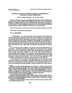
be seen on Table 3 (on right). This is also clear in Figure 1, which plots the SSP coefficients of methods of nonlinear order p = 2 (and therefore of p = 3 as well) and p = 4 with different linear orders 3 ≤ pin ≤ 9. In this figure we observe that if we compare methods with a given plin , the SSP coefficient of the methods with nonlinear order p = 2 in does not have significantly higher SSP coefficient than the methods with nonlinear order p = 4. This would seem to suggest that the linear order is the main constraint on the SSP coefficient, as was the case for the explicit methods in [10]. However, Figure 2, which looks at methods with higher nonlinear orders p = 5 and p = 6 tells a different story. In this figure we compare three methods compare three methods with linear order plin = 5 and nonlinear orders p = 2, 4, 5 (in blue solid, dot-dashed with circle marker, and dashed with + markers) and similarly, three methods with linear order plin = 6 and nonlinear orders p = 2, 4, 6 (in red solid, dot-dashed with circle marker, and dashed with + markers) We say that in this case, as we go to higher nonlinear orders the SSP coefficient is significantly reduced. For example, a six stage (s = 6) sixth nonlinear order method has an SSP coefficient C = 0.18 whereas the six stage LNL method with nonlinear order p = 4 and linear order plin = 6 has an SSP coefficient C = 5.14. The SSP coefficients of the implicit SSP LNL Runge–Kutta methods in 3 should be compared to those of the explicit SSP LNL Runge–Kutta methods 2. we see that the implicit methods have SSP coefficients that are significantly larger than the corresponding explicit methods: up to six times larger. This suggests that the cost of the implicit solver may be offset by the larger allowable time-step in some cases. While the methods in this section are not necessarily suitable for every application, they are valuable in that they provide an upper bound on the possible SSP coefficient for a given number of stages and linear and nonlinear orders, and demonstrate the effect of increasing the nonlinear order.
8
s\plin 3 4 5 6 7 8 9
Implicit p = 2, p = 3 methods 4 5 6 7 8 3.24 – – – – 4.56 3.64 – – – 6.15 5.01 3.97 – – 7.85 6.66 5.17 4.27 – 9.60 8.42 6.54 5.51 4.54 11.23 10.21 7.92 6.91 5.82 12.81 11.82 9.48 8.33 7.03
9 – – – – – 4.79 6.10
4 2.05 4.42 6.04 7.80 9.19 10.67 12.04
Implicit p = 4 methods 5 6 7 8 3.54 – – – 4.63 3.81 – – 6.49 5.14 4.14 – 7.86 6.42 5.42 4.46 9.25 7.86 6.82 5.80 11.15 9.46 8.32 6.98
9 – – – – 4.74 6.08
Table 3: The value of C for LNL iRK with linear order plin , and nonlinear order p = 2 on left and p = 4 on right. Note along the diagonal these the SSP coefficients are close to six times larger than the corresponding explicit LNL methods.
2.2.1
Coefficients of selected optimal methods
The coefficients of all the methods listed in the section above can be downloaded as .mat files from [5]. In this section we list, for the user’s convenience, the non-zero coefficients of three methods of particular interest. We use the canonical Shu–Osher form here, where all the forward-Euler steps are of the same size ∆t r and r = C: y
(i)
un+1
s X
� � ∆t (j) (j) F (y ) , i = 1, ..., s = vi u + αi,j y + r j=1 � � s X dt n (j) (j) = vs+1 u + αs+1,j y + βs+1,j F (y ) , r n
(11)
j=1
SSP iRK LNL p = 4, s = plin = 6: One of the most efficient method produced was the s = plin = 6 LNL method of nonlinear order p = 4 that has SSP coefficient C = 5.138. The corresponding implicit Runge–Kutta method in [11] which has s = p = plin = 6 has a much smaller SSP coefficient of C = 0.18. The non-zero coefficients are: α1,1 α2,1 α2,2 α3,2 α3,3 α4,3 α4,4
= 0.227696764527492, = 0.773299008278988, = 0.226700991721012, = 0.566850708114719, = 0.245119620891410, = 0.589123375926120, = 0.245088907884392,
α5,2 α5,4 α5,5 α6,5 α6,6 α7,1 α7,2
= 0.273146312340082, = 0.468182990851259, = 0.226105041192215, = 0.772671881656312, = 0.227328118343688, = 0.005835455470528, = 0.016317087005175,
α7,3 = 0.140604847510042, α7,4 = 0.134029552181827, α7,6 = 0.703213057832428, v1 = 0.772303235472508, v3 = 0.188029670993872, v4 = 0.165787716189488, v5 = 0.032565655616444,
SSP iRK LNL p = 4, s = 8, plin = 9: A very high order LNL method with s = 8, plin = 9, and p = 4 has SSP coefficient C = 4.735. This method has the following non-zero coefficients 9
14
12
P=2 P =5
P lin =4
lin
P=4 P =5 lin
P lin =5
12
P=5 P lin =5
10
P=2 P lin =6 P=4 P lin =6
P lin =7
10
SSP Coeficient
SSP Coeficient
P lin =6
P lin =8 P lin =9
8
6
6
4
2
4
2
P=6 P lin =6
8
0
3
4
5
6
Stages
7
8
9
4
4.5
5
5.5
6
6.5
Stages
7
7.5
8
8.5
9
Figure 2: Comparison of SSP coefficients of methods with linear order plin = 5 (blue) and plin = 6 (red) for several nonlinear orders. The p = 2 lines are solid, p = 4 lines are dot-dashed with circle marker, and p = plin lines are dashed with + markers. Clearly, the SSP coefficient of methods with the same number of stages and linear order is significantly smaller for larger nonlinear orders.
Figure 1: SSP coefficients of methods with nonlinear order p = 2 (solid lines) and nonlinear order p = 4 (dashed lines) for linear orders 4 ≤ plin ≤ 9, for increasing stages. We note that the SSP coefficients of p = 2 and p = 3 are close too identical for all methods with s stages, and are not significantly different for the two nonlinear orders p = 2 and p = 4, and get closer as s increases. given in the canonical Shu-Osher form (11): α1,1 α2,1 α2,2 α3,2 α3,3 α4,3 α4,4
= 0.146943975728437, = 0.854796464970015, = 0.145203535029985, = 0.612204675611763, = 0.136155301978034, = 0.742598809241823, = 0.135251383179389,
α5,4 α5,5 α6,1 α6,5 α6,6 α7,2 α7,6
= 0.796548121452431, = 0.136561808924711, = 0.260577803576825, = 0.269626835933091, = 0.206284522717965, = 0.198036604411651, = 0.596122990527354,
α7,7 α8,5 α8,7 α8,8 α9,1 α9,2 α9,4
= 0.205840405060996, = 0.510718712707677, = 0.353463620808626, = 0.135817666483696, = 0.003486997034287, = 0.067521279383993, = 0.256478057637965,
α9,8 = 0.662855611847356, v1 = 0.853056024271563, v3 = 0.251640022410203, v4 = 0.122149807578787, v5 = 0.066890069622858, v6 = 0.263510837772119, v9 = 0.009658054096400,
SSP iRK LNL p = 2, s = 10, plin = 11: A very high order LNL method with s = 10, plin = 11, and p = 2 has SSP coefficient C = 5.2306. This method has a very low storage form, where the non-zero coefficients are given in the canonical Shu-Osher form (11):
10
α1,1 α2,1 α2,2 α3,2 α3,3 α4,3 α4,4 α5,4
2.3
= 0.193277114534410, = 0.806723199562524, = 0.193276800437476, = 0.080009844643863, = 0.129448616881864, = 0.870552299752962, = 0.129447700247038, = 0.241978799620415,
α5,5 α6,5 α6,6 α7,6 α7,7 α8,7 α8,8 α9,8
= 0.117235708890556, = 0.718962893859175, = 0.117234259419046, = 0.546025511754727, = 0.117237564101546, = 0.760604303914880, = 0.117233906332291, = 0.822633852616330,
α9,9 = 0.117235191356250, α10,9 = 0.880317745035338, α10,10 = 0.117236158521012, α11,1 = 0.028409070825259, α11,2 = 0.043364313791996, α11,3 = 0.001158601801210, α11,10 = 0.921532831100178, v1 = 0.806722885465590,
v3 = 0.790541538474273, v5 = 0.640785491489029, v6 = 0.163802846721778, v7 = 0.336736924143727, v8 = 0.122161789752829, v9 = 0.060130956027420, v10 = 0.002446096443650, v11 = 0.005535182481357,
Optimizing for Additional Properties
In the section above we optimized the implicit Runge–Kutta methods for the largest possible SSP coefficients. However, in many cases the motivation for using an implicit method is not only the SSP coefficient; this is especially true in cases where the additional time-step allowed for the implicit SSP methods is not enough to offset the cost of the implicit solver needed. If we wish to optimize for other properties, such as linear stability regions, alongside the SSP property, we can add a condition to the inequality constraints in the optimization routine. The methods we found above did not have large linear stability regions, and so we wish to explore whether one can find methods that have a large SSP coefficient as well as large linear stability region. In this section we present our optimized methods using this approach. The resulting methods are suboptimal in terms of SSP coefficients but benefit, as desired, from larger regions of absolute stability. In Figures (3) and (4) we show the linear stability regions of methods found from this co-optimization approach compared to those found in the subsection above. Figure (3) shows several five stage (s = 5) methods with p = 3 and plin = 4 resulting from optimization runs that required increasing linear stability regions that included more of the real axis. We show four methods: in blue is the linear stability of the optimal SSP method in the subsection above. This method has SSP coefficient C = 6.1472, and crosses the negative real axis at x = −26.3. In red is the linear stability region of a method that has SSP coefficient C = 5.9537 but allows slightly more of the negative real axis, crossing it at x = −29.766. Next, in green is the linear stability of a method with a slightly smaller SSP coefficient of C = 5.6249 but which allows much more of the negative real axis, crossing it at x = −56.247. Finally, in black is the linear stability region of a method with C = 5.4459 but which allows significantly more of the negative real axis, crossing it at x = −81.68. Thus we see that we can co-optimize for additional linear stability properties while balancing the need for a large SSP coefficient. Another frequently desirable feature of time-stepping methods is that they include the imaginary axis or points near the imaginary axis. This is particularly desirable when solving hyperbolic PDEs. In our case, the optimal SSP five stage (s = 5) method with p = 3 and plin = 4 does not include the imaginary axis at all (y = 0). Even when we consider the close neighborhood of the imaginary axis (points which are closer than 10−5 to the imaginary axis) it only allows these values up to a value of y = .9099. Figure (4) shows the linear stability of this region in blue. If 11
we wish to increase these values, we can obtain a method whose linear stability region is shown in red. This method clearly captures much less of the real axis, but it includes the imaginary axis up to the value of y = 5.28. The zoomed image of the region of linear stability in Figure (4) shows this difference clearly. The SSP coefficient of the second method is significantly less, at C = 4.1322, but this may be a worthwhile trade-off where needed. The methods in this subsection are meant to represent a small slice of the range of possible properties for which one may co-optimize. As in [27], it is possible to optimize SSP methods for particular linear stability regions, and it is also possible to consider other desirable properties with respect to which we can to co-optimize. Furthermore, other optimization routes are possible, such as starting with a known linear stability polynomial or a particular form of a method that is known to have desirable properties.
20
30 20
9
R = 6.1472
R = 6.1472 R = 5.9537 R = 5.6249 R = 5.4459
R = 4.1322 15
8
10
7
10
5
0
0
-10
-5
-20
-10
-30
-15
6 5 4 3
-100
-80
-60
-40
-20
0
-20 -30
2 1 0 -25
-20
-15
-10
-5
0
0
1
Figure 3: Linear stability regions in the complex plane
Figure 4: Linear stability regions in the complex plane
of the optimal SSP method (blue line) and co-optimized methods (in red, green, and black) with increasing real axis linear stability. Shown in the legend are the values of the SSP coefficients for these methods.
of the optimal SSP method (blue line) and co-optimized methods in red with larger imaginary axis linear stability, but at the cost of a smaller real axis region and SSP coefficient. On the right is the same image zoomed in on the Imaginary axis.
2.4
Numerical Results
The methods above were found by the optimization code [5], where the order conditions are imposed as equality constraints. It is a good idea to check that the methods indeed perform as designed on a series of linear and nonlinear test cases. These convergence studies are reported in Section 2.4.1. Next, we wish to test how the methods perform in terms of the predicted SSP time-step. Clearly, the SSP coefficient gives a guarantee that the desired property is pre12
served by the time-stepping method at the corresponding time-step. In Section 2.4.2 we study the difference between the guaranteed time-step and the actual time-step at which the desired nonlinear stability property (in this case the total variation diminishing property) still holds. A close agreement between these two time-steps demonstrates the relevance of the SSP property for typical cases. 2.4.1
Verification of the linear and nonlinear orders of convergence
Example 1.1: Study of the convergence rate for a nonlinear ODE To verify the nonlinear order of the implicit Runge–Kutta methods with nonlinear order p and linear order plin we us a nonlinear system of ODEs u01 = u2 u02 = 1� (−u1 + (1 − u21 )u2 )
(12)
known as the van der Pol problem. We use � = 10 and initial conditions u0 = (0.5; 0). This problem was tested with methods with number of stages s, linear order plin and nonlinear order p. Each methods is designated by (s, plin , p). Of each nonlinear order we test two methods: one with low stages and plin = p and one with high number of stages and linear order. The methods we test are (s, plin , p) = (2, 2, 2), (7, 7, 2), (3, 3, 3), (7, 7, 3), (4, 4, 4), (7, 7, 4). We use 1 1 1 1 1 ∆t = 250 , 350 , 450 , 550 , 650 and step forward to time Tf inal = 1.0. The errors are calculated by using a very accurate solution calculated by MATLAB’s ODE45 routine with tolerances set to AbsTol=RelTol= 10−14 . In Figure 5 we show that the log10 of the errors in the first component vs. the log10 of the time-step ∆t. The orders (slope of the line) are taken by taking a linear fit using MATLAB’s polyfit. We observe the rate of convergence expected for the nonlinear order of the method. Example 1.2: Study of the convergence rate for a linear PDE To verify the linear order of convergence of these methods we solve a linear advection problem Ut + Ux = 0 with periodic boundary conditions and initial conditions U0 (x) = sin(x) on the spatial domain x ∈ [0, 2π]. We discretize the spatial grid with N = 11 equidistant points and use the Fourier pseudospectral differentiation matrix D [14] to compute F ≈ −Ux . In this case, the solution is a sine wave, so that the pseudospectral method is exact, and the spatial discretization contributes no errors. For this reason, we use grid refinement in time only, and use a range of time steps, ∆t = λ∆x where 1 2 3 4 5 6 7 8 9 λ = 10 , 10 , 10 , 10 , 10 , 10 , 10 , 10 , 10 to compute the solution to final time Tf = 5.0. The errors are measured in the `2 norm. Two methods from each order were tested for convergence on this problem. In Figure 7 we show the convergence plots for the s = plin methods the s = plin − 1 methods, both with nonlinear order p = 4. The slopes were measured in the region before round-off error dominates. We observe that the design-order plin of each method for linear problems is apparent.
13
-2
-4
-5 -3 -6 -4
Log 10(Error)
Log 10(Error)
-7
-8
-9
-5
-6
-10
-12
-13 -2.85
-7
(2,2,2) m=2.00 (7,7,2) m=2.00 (3,3,3) m=3.01 (7,7,3) m=2.97 (4,4,4) m=3.98 (7,7,4) m=3.88
-11
-2.8
-2.75
-2.7
-2.65
-2.6
-2.55
-2.5
-2.45
-2.4
(2,2,2) m=1.98 (7,7,2) m=1.93 (3,3,3) m=2.98 (7,7,3) m=2.96 (4,4,4) m=4.11 (7,7,4) m=4.06
-8
-9 -1.8
-2.35
-1.6
Log 10(∆t)
-1.4
-1.2
-1
-0.8
-0.6
-0.4
Log 10(∆t)
Figure 5: Convergence study in Example 1.1, the nonlinear van der Pol problem. Methods tested are (s, plin , p) = (2, 2, 2), (7, 7, 2), (3, 3, 3), (7, 7, 3), (4, 4, 4), (7, 7, 4), using time-step ∆t = 1 1 1 1 1 250 , 350 , 450 , 550 , 650 to step forward to time Tf inal = 1.0. The rate of convergence is, as predicted, the designed nonlinear order of the method.
Figure 6: Convergence study in Example 1.3, the Buckley-Leverett problem. Methods tested are (s, plin , p) = (2, 2, 2), (7, 7, 2), (3, 3, 3), (7, 7, 3), (4, 4, 4), (7, 7, 4), using time-step ∆t = λ∆x 1 1 with λ = 12 , 14 , 18 , 16 , 32 , and spatial step ∆x = π4 to step forward to time Tf inal = 2.0. The slopes of the lines show the desired order of accuracy.
Example 1.3: Study of the convergence rate for a nonlinear PDE To verify the nonlinear order on PDE, we solve the Buckley-Leverett equation which is commonly used to model twophase flow through porous media: ut + f (u)x = 0,
where f (u) =
u2 , u2 + a(1 − u)2
on x ∈ [0, 2π], with periodic boundary conditions. We take a = 31 and initial condition u(x, 0) = sin(x). For the spatial discretization, we use a Fourier pseudospectral method as above. ∆t = 1 1 1 1 1 λ∆x with λ = 32 , 16 , 8 , 4 , 2 , and ∆x = π4 , evolved to final time T = 2.0. The errors are calculated by using a very accurate solution calculated by MATLAB’s ODE45 routine with tolerances set to AbsTol=RelTol= 10−14 . In Figure 6 we show that the log10 of the errors in the first component vs. the log10 of the time-step ∆t. The orders (slope of the line) are taken by taking a linear fit using MATLAB’s polyfit. We observe the rate of convergence expected for the nonlinear order of the method. 2.4.2
Verification of the SSP property
Example 2: The methods above are selected to optimize the SSP coefficient C. This value guarantees that the desired strong stability property that is satisfied by the forward Euler method 14
Figure 7: Convergence study in Example 1.2, the linear advection problem with pseudospectral differentiation of the spatial derivatives. Here we use N = 11 equidistant points between (0, 2π), and ∆t = λ∆x. The solution is evolved forward to time Tf = 5.0. Convergence plots for linear methods with s = plin (left) and s = plin − 1 (right). The slopes of the lines are calculated before round-off error ruins the convergence.
will be preserved under the condition ∆t ≤ C∆tFE . It is interesting to see whether for typical problems this value is predictive of the actual time-step at which the desired strong stability properties are violated. As an example, we consider the linear advection equation Ut + Ux = 0, on the domain x ∈ [−1, 1] with periodic boundary conditions and the step function initial condition � 1 −0.1 ≤ x ≤ 0.1 U0 (x) = 0 otherwise We approximate the spatial derivative with a first order finite difference method, which is total variation diminishing (TVD) for all values ∆t ≤ ∆x. This simple example is chosen as our experience has shown [11] that this problem often demonstrates the sharpness of the SSP time1 step. For all of our simulations, we use a fixed grid of size ∆x = 300 , and a time-step ∆t = λ∆x, where we choose values of λ starting from the minimum of C/10 or 0.1. We then increase the value of λ until the TVD property is violated. To measure the effectiveness of these methods, we consider the maximum observed rise in total variation defined by � max kun+1 kT V − kun kT V . (13) 0≤n≤N −1
over the first N = 20 steps. We are interested in the time-step in which this rise becomes evident, so we consider a violation if the TV rises 10−10 or more at any time-step. The value of λ for which this violation in TV occurs is refined to the level of 10−12 . In Figure 8 we plot the maximal ∆t rise in total variation over different values of λ = ∆x for a selection of methods. It is interesting 15
SSP Test 6s5p Methods R Linear =6.6637
0
Linear 3pLNL 4pLNL
-4
-6
-8
-10
-12
-14
-16
Linear 3pLNL 4pLNL
-2
Log10 of Maximum Violation of Total Variation
Log10 of Maximum Violation of Total Variation
-2
SSP Test 6s6p Methods R Linear =5.1744
0
-4
-6
-8
-10
-12
-14
0
1
2
3
4
5
6
-16
7
0
1
2
∆t ∆x
3
4
5
6
∆t ∆x
Figure 8: The observed rise in total variation over the first 20 steps for the s = 6, plin = 5 methods (left) and the s = 6, plin = 6 methods. to observe that the change in behavior of the methods is quite sharp – once a certain threshold is reached, the SSP coefficient goes from being very small (< 10−14 ) to being much larger (> 10−4 ) with small changes in the time-step. We are also interested in difference between the predicted and observed value of C (or equivalently, ∆t) at which this violation happens. Table 4 provides these values for the case p = 2. We observe that for all the methods with p = 2 and plin < s, the observed time-step for which the TVD property is preserved matches the predicted time-step up to ≈ 10−10 . For these cases, the SSP coefficient is an excellent predictor of the actual value for which the TVD property breaks down. s\plin 2 3 4 5 6 7 8 9
2 2.5×10⁻¹² 4.0×10⁻¹² 8.1×10⁻¹² 1.6×10⁻¹¹ 3.2×10⁻¹¹ 6.4×10⁻¹¹ 1.2×10⁻¹⁰ 2.5×10⁻¹⁰
3 1.5×10⁻¹² 2.5×10⁻¹² 4.5×10⁻¹² 9.1×10⁻¹² 1.8×10⁻¹¹ 3.7×10⁻¹¹ 7.4×10⁻¹¹ 1.5×10⁻¹⁰
4
5
6
7
8
9
3.8×10⁻² 2.2×10⁻¹¹ 1.2×10⁻¹¹ 1.1×10⁻¹¹ 1.4×10⁻¹¹ 3.7×10⁻¹⁰ 1.4×10⁻¹⁰
6.4×10⁻² 7.6×10⁻¹² 6.6×10⁻¹² 7.6×10⁻¹² 1.0×10⁻¹¹ 1.7×10⁻¹⁰
1.7 ×10⁻¹ 2.6×10⁻¹¹ 2.6×10⁻¹⁰ 5.5×10⁻¹¹ 3.4×10⁻¹¹
3.0×10⁻¹ 7.1×10⁻¹² 5.5×10⁻¹¹ 2.1×10⁻¹¹
3.6×10⁻¹ 1.4×10⁻² 2.2×10⁻¹⁰
4.7×10⁻¹ 3.4×10⁻²
Table 4: The difference between the theoretical and observed SSP coefficient at which the maximal rise in total variation is about the threshold of 10−10 for the p = 2 methods.
16
For the cases where plin = s ≤ 7, and p = 2, the observed time step is also within ≈ 10−10 of the predicted value. This is true also for the methods with p = 3. However, when plin = s = 8, 9, and p = 2, 3, 4, the observed time step is much larger than the predicted time-step (≈ 10−1 or 10−2 ). Also, for p = 4, the s = plin = 5, we also have a larger difference between the observed and predicted time-step. Finally, in the cases where s = plin −1, the observed time step is usually much larger than the predicted time-step (≈ 10−1 or 10−2 ), and the SSP coefficient is not sharp at all.
3
Optimal SSP IMEX Runge–Kutta methods with plin ≥ p
For cases in which the problem has a linear component which restricts the time-step significantly, and a nonlinear component which does not, it may be advantageous to treat the two components differently by using an implicit-explicit method. Consider an initial value problem of the form U 0 (t) = f (U (t)) + g(U (t)),
U (t0 ) = U0
t ≥ t0
(14)
which is semi-discretized to give an ODE of the form u0 (t) = F (u) + G(u).
(15)
To step the two components forward in time, one explicitly and one implicitly, we use an ImplicitExplicit (IMEX) Runge–Kutta method, which is a particular kind of additive Runge–Kutta method. An s-stage Additive Runge–Kutta (ARK) method is defined by two s × s real matrices ˜ such that: ˜ and two real vectors b, b A, A u(i) = un + ∆t
s X
aij F (u(j) + ∆t
j=1
un+1 = un + ∆t
s X i=1
s X
a ˜ij G(u(j) )
i = 1, . . . , s
j=1
bi F (u(i) + h
s X
˜bi G(u(i) ),
(16) i = 1, . . . , s.
i=1
We select A to be a strictly lower triangular matrix, so that this additive Runge–Kutta method contains an explicit method (represented by (A, b)) used for the non-stiff part F . As above, we ˜ to be a lower triangular matrix, limit ourselves to diagonally implicit methods and require A ˜ represents an implicit Runge–Kutta (DIRK) method used for the stiff part G, as ˜ b) where (A, in [18, 2, 20]. IMEX methods were first introduced by Crouziex in 1980 [7] for evolving parabolic equations. In 1997, Ascher, Ruuth, and Wetton [1] introduced IMEX multi-step methods for time dependent PDEs, notably convection-diffusion equations, and in the same year Ascher, Ruuth and Spiteri [2] presented the IMEX Runge–Kutta schemes for such problems. Although the authors were not focused on designing SSP pairs, some of methods are in fact known SSP methods. For example, 17
the method in [2, Section 2.4] is the midpoint explicit and implicit SSP methods. In this work, all the implicit methods are SDIRK methods, and most have nice properties such as L-stability, with diagonal values γ that are those mentioned in the books of Hairer, Norsett, and Wanner [12, 13]. Implicit methods are often particularly desirable when applied to a linear component. In this case, the order conditions simplify. In [4], Calvo, Frutos, and Novo developed IMEX pairs for the case where the implicit component G is linear. This was the first work where the linear and nonlinear orders were separated. The methods they produced had nonlinear implicit order pim = 2, nonlinear explicit order and linear order pex = plin = 3, 4. Kennedy and Carpenter [20] derived IMEX Runge–Kutta methods based on singly diagonally implicit Runge–Kutta (SDIRK) methods. This work introduced sophisticated IMEX methods with good accuracy and stability properties, as well as high quality embedded methods for error control and other features that make these methods usable in complicated applications. The first IMEX methods that had SSP properties were considered by Pareschi and Russo in [29]. In this work, explicit SSP Runge–Kutta methods L-stable implicit components. These schemes were designed to be asymptotically preserving. The authors listed a pex = pim = p = 3 order conditions, and also presented a table depicting the number of coupling conditions under each underlying assumptions. In this work, the authors designed their methods while enforcing ˜. They the condition that the abscissas of the explicit and implicit methods were equal c = c ˜ ˜ and b = b the coupling conditions were redundant observed that under the assumption c = c for the p = 3. It is worth noting the SDIRK implicit pairs from [29] have the same γ value listed in the books of Hairer, Norsett, and Wanner [12, 13]. Further work by Boscarino, Pareschi, ˜ In this and Russo [3] observed that the order reduction phenomenon disappears when b = b. work they presented a globally stiffly accurate, third order method with non-negative explicit coefficients (named BPR(3,5,3). Higueras [17] was first to consider SSP IMEX methods where both explicit and implicit pairs of the methods were SSP. In this work, she presented conditions for an IMEX Runge–Kutta methods to be SSP, and listed some previously known methods, such as methods from [2], that satisfy the SSP conditions. The methods that appear in this work are of order p ≤ 3, and there is no distinction made between the explicit, implicit and linear order of the methods. In [18] Higueras presented order barriers and other characteristics of strong stability preserving additive Runge–Kutta methods. This work contains several very important properties of SSP IMEX pairs and is necessary to the understanding of the structure of these methods. In later work, [28] several known methods were analyzed in terms of their linear stability region and SSP performance on astrophysics-type problems. The implicit second order methods considered are L-stable (and thus A-stable as well), but the third order method was not A-stable. In their work in [19], the authors mainly focused on second order, three-stage explicit methods that implicit SSP pairs. In this work, the main focus was on methods with suboptimal SSP coefficients that offered significant additional benefits (including large linear stability regions). 18
Our approach to deriving optimal SSP methods is slightly different from [17, 19]. First, we use a slightly different formulation of the SSP condition, which facilitates the construction of an optimization problem. Next, we introduce a coefficient which relates the strong stability condition of F to that of G, and make an observation about time step of optimal methods using this coefficient, which also simplifies the optimization routine. But the main distinction between our work and prior work is the fact that our investigations focus on higher order methods, and especially methods with higher linear order. To analyze an IMEX method in the SSP context, we assume as in [17, 19] that when each component (F or G) of the ODE is stepped forward individually with a forward Euler method, the new solution will satisfy a strong stability property in some desired convex functional k · k, but under very different time-step restrictions: kun + ∆tF (un )k ≤ kun k,
0 ≤ ∆t ≤ ∆tF E ,
(17)
0 ≤ ∆t ≤ K∆tF E .
(18)
and kun + ∆tG(un )k ≤ kun k,
If K is small, the G component will make the overall allowable time-step of the method very small, so it may be worthwhile to treat this component implicitly. We know [24, 11] that the allowable time-step for an s-stage SSP implicit Runge–Kutta method of order p > 1 can only be expected to be, at most, 2s times the allowable explicit forward Euler time-step ∆tFE , which does not typically offset the additional cost of solving the implicit system. However, in the previous discussions we show that the allowable time-step of an implicit method is in fact more than twice, and in the new methods presented in Section 2 up to six times, as large as that of an explicit method with the same order and number of stages and order. Furthermore, in the case where G is a linear operator, the cost of the implicit solver is much smaller and under such circumstances it may be worthwhile to use an implicit SSP Runge–Kutta method for this part of the problem. However, if F is nonlinear, or if for any other reason the cost of implicitly solving the system for F is large, we wish to use an explicit time-stepping method for this part. The IMEX approach may also be desirable if the value of K is not small (perhaps even infinitely large) but other factors, such as linear stability requirements, greatly limit the step size if G is treated explicitly. The main contribution of our work is to present SSP IMEX methods with plin ≥ 4. These methods have not appeared in the literature, and while it is not clear yet how useful they will be in actual applications, we believe that understanding the SSP bounds on such methods and its dependence on the linear and nonlinear orders is of value.
3.1
Formulating the Optimization Problem
To formulate the optimization method for this problem, we stack the matrix A and the vector b, padded with zeroes, into a square matrix S (as we did in Equation (9)). Similarly, we convert 19
˜ into a matrix S. ˜ and b ˜ We now rewrite the method (16) as A ˜ Y = eun + ∆tSF (Y ) + ∆tSG(Y ).
(19)
Now, we add the terms �
� ˜ Y I + rS + r˜S Y
where
�
� � � ∆t ∆t ˜ = eu + rS Y + F (Y ) + r˜S Y + G(Y ) , r r˜ � � � � ∆t ∆t n F (Y ) + Q Y + G(Y ) , = R(eu ) + P Y + r r˜ n
� �−1 ˜ , R = I + rS + r˜S
P = rRS,
˜ Q = r˜RS.
From this formulation we see that if Re, P , and Q are all positive component-wise, then the resulting method is simply a convex combinations of forward Euler steps Y + ∆t r F (Y ) and ∆t Y + r˜ G(Y ), and therefore will preserve the strong stability property in the desired convex functional k · k, under the time-step restriction ∆t ≤ min (r∆tFE , r˜K∆tFE ). We observe that the optimal methods will have r = r˜K, so the optimization problem becomes: Maximize r such that � r ˜ �−1 I + rS + S e≥0 (20a) K � � r ˜ −1 S≥0 (20b) r I + rS + S K r ˜ �−1 ˜ r � I + rS + S S≥0 (20c) K K ˜ = 0 for k = 1, ..., P, ˜ b) τk (A, b, A, (20d) ˜ are the order ˜ b) where the first three inequalities are understood component-wise, and τk (A, b, A, conditions, described in the sections below. This optimization gives the Butcher coefficients A, ˜ and an optimal value of the SSP coefficient C = r. Of course, for each value of K, ˜ and b, b, A, a different method will be optimal. Note that although this process defines a sufficient condition for the resulting method to be SSP with SSP coefficient C = r, there is no reason to expect this condition to be necessary. In particular, this formulation ignores the possible interactions between F and G that would result in more relaxed SSP conditions. Once again, the order conditions (20d) are a key piece of the optimization, and serve as equality constraints. These conditions will be described in the next two subsections.
20
3.1.1
Linear Order Conditions
First order plin = 1: The order conditions for an additive method (16) to be first order are ˜ T e = 1. b
bT e = 1,
(21)
This has two conditions: one for the explicit part and one for the implicit part. To generalize ˜ T }, and the order conditions become these order conditions, we define Φ1 = {φ1,1 , φ1,2 } = {bT , b T T ˜ b e = 1, b e = 1. ˜ = {φ1,1 A, φ1,1 A, ˜ φ1,2 A, φ1,2 A}, ˜ and the Second order plin = 2: Define Φ2 = Φ1 ⊗ {A, A} 1 order conditions are each of these right-multiplied by e and set equal to 2 . Recall that c = Ae ˜ The order conditions then become ˜ = Ae and c 1 ˜T 1 ˜T 1 1 ˜= , b ˜= . c= , b c bT c = , bT c 2 2 2 2 ˜ and right-multiply by e to obtain: Third order plin = 3: use Φ3 = Φ2 ⊗ {A, A} 1 ˜T bT Ac = , b A˜ c= 6 ˜ T A˜ ˜ = 1, b ˜c = bT Ac 6 To obtain higher linear order, we define
1 ˜T 1 , b Ac = , bT A˜ c= 6 6 1 ˜T ˜ 1 ˜c = , b Ac = , bT A˜ 6 6
1 , 6 1 . 6
˜ = {φq,1 A, φq,1 A, ˜ φq,2 A, φq,2 A, ˜ ...φq,2q A, φq,2q A} ˜ Φq = Φq−1 ⊗ {A, A} and the resulting new order conditions for this order take the form φq,j e =
1 e q!
∀q, j.
To go from linear order plin = q − 1 to linear order plin = q we require an additional 2q order conditions. We observe that unlike in the implicit case, in the IMEX case the number of order conditions grows very rapidly even when both F and G are linear. This is due to the many coupling order conditions that are required for the two components to interact properly. 3.1.2
Nonlinear Order Conditions
The order conditions for first and second order are the same for both linear and nonlinear problems. In this section, we look at the order conditions for nonlinear orders pe = 3, 4 for the explicit part and pi = 3, 4 for the implicit part. Nonlinear order p = 3: For third order, we have the linear order conditions for the explicit and implicit parts, and the nonlinear coupling conditions given in the section above. In addition, we have the following nonlinear condition on the explicit part: 1 bT c 2 = , 3 21
(22a)
the nonlinear conditions on the implicit part, 1 ˜T c ˜2 = b 3
(22b)
and the nonlinear coupling conditions 1 bT C˜ c= , 3
˜c = bT C˜
1 3
(22c)
˜ T Cc = 1 , b 3
˜ T Cc ˜ = 1. b 3
(22d)
When we wish to have pe = 3 but use a linear G (i.e pi = 2) we need to include all the linear order conditions for plin = 3, as well as the nonlinear equations for the explicit part (22a), and we must include the coupled order conditions in (22c). We can neglect the nonlinear implicit conditions (22b) and (22d). Nonlinear order p = 4: We include all the linear and nonlinear order conditions above, for the explicit and implicit parts as well as the coupled conditions. In addition, we have the nonlinear order condition Equation (23a) for the explicit method: 1 1 , bT c3 = , 12 4 The nonlinear order condition for the implicit part is bT Ac2 =
˜ T A˜ ˜ c2 = 1 , b 12
1 ˜T c ˜3 = , b 4
1 bT CAc = . 8
(23a)
˜T C ˜ c = 1. ˜ A˜ b 8
(23b)
And the nonlinear coupled order conditions 1 ˜ = 1, ˜ c = 1 , bT CCc ˜ = 1 , bT CC˜ ˜ c = 1 , bT C ˜ C˜ ˜ c = 1 , bT CAc , bT AC˜ 12 12 4 4 4 8 1 1 1 1 1 1 T T T T T T ˜ c = , b CA˜ ˜ = , b C ˜c = , ˜ ˜ c= , b C ˜ Ac ˜ A˜ b CA˜ c = , b CAc = , b CA˜ 8 8 8 8 8 8 bT AC˜ c=
(24)
1 1 ˜ T ACc ˜ T AC˜ ˜ T ACc ˜ ˜ c = 1 , bT A ˜ C˜ ˜ ˜c = 1 , b ˜ = 1, b ˜c = 1 , b , bT AC˜ = , bT ACc = 12 12 12 12 12 12 ˜ T AC˜ ˜ T ACc = 1 , b ˜ T CCc ˜ T CC˜ ˜ T CCc = 1 , b ˜ T CAc ˜ c= 1 , b ˜ = 1, ˜ = 1, b ˜c = 1, b (25) b 12 12 4 4 4 8 1 1 ˜ T CA˜ ˜ T CA˜ ˜ T CAc ˜ T CA˜ ˜T C ˜ T CAc = 1 , ˜ = 1, b ˜ c = 1, b ˜ ˜ c = 1, b ˜ Ac b c= , b = , b 8 8 8 8 8 8
In the case where G is linear and we wish to have pi = 2, we must satisfy all the linear order conditions, the nonlinear explicit conditions (23a), and the coupling conditions (24), but we can neglect the nonlinear implicit conditions (23b) and the nonlinear coupling conditions (25)
22
3.2
Optimal SSP IMEX Methods
We formulate the optimization problem above in a MATLAB routine following [25] and use it to generate optimized methods for different choices of K. We focus primarily on cases in which the number of stages s is the same as the linear order plin or a little larger. The nonlinear orders of interest are p = 2, 3, 4. We note that in finding optimal methods, we frequently observed convergence to higher order than we required or expected. For example, in the case where we ˜ and c = c ˜, as we only require pi = 2 and pe > 2 the optimal SSP methods generally have b = b would expect from [18] and due to this the nonlinear implicit order is higher than required, pi = 3. However, we also find that in some cases we required only pi = 2 and pe = 4, but the methods converged to pi = pe = 4. For this reason, in the following sections we describe mostly optimal methods that have p = pi = pe (though some exceptions exist as is noted below). In some cases, especially where the number of stages s is large and where there are more order constraints, the optimization routine had difficulties converging and we are not comfortable stating that the methods found are optimal. For this reason, we refer to the methods as optimized rather than optimal. IMEX pairs for K = ∞ First, we look at the case where there is no constraint resulting from the G component, which is equivalent to setting K = ∞. We reformulate the optimization ˜ terms in (20a) – (20c). The case of K = ∞ is problem to account for this by shutting off the S equivalent to the case where the implicit method is non-SSP while the explicit method is SSP. In many such cases, researchers have focused on finding methods where the explicit component is SSP and the implicit component is A-stable, L-stable, or stiffly stable. These methods were mostly of order p ≤ 3 with few p = 4 methods. It is known from the order barrier on explicit SSP Runge–Kutta methods that methods of order p > 4 cannot exist. In our case, we focus primarily on methods that have plin ≥ 4. We first study methods with plin ≥ p, and we do not optimize for linear stability: our rationale for studying these methods is to demonstrate that where there is no SSP constraint on G we are able to find implicit pairs for optimal explicit SSP methods for F . Using our optimization routine we found methods with s stages, linear order plin and nonlinear orders p = pi = pe = 2, 3 with K = ∞ with s = plin , plin + 1, plin + 2. Initially, we imposed a non-negativity conditions on all the coeffiicents, and were able to find many good methods. Later, we relaxed this condition and ˜ which allowed us to find additional methods. Table 5 contains allowed negative coefficients in S, the SSP coefficients of these methods, which clearly match those of the explicit LNL SSP Runge– Kutta methods found in [10] and repeated in Table 2. The SSP coefficients of methods that have ˜ are listed in bold. These methods do not have large linear stability regions, negative values in S as they were not optimized for this purpose. However, these results show that the addition of an implicit component that does not have its own SSP constraint does not have an adverse effect on the size of the SSP IMEX method despite the addition of many new order conditions (coupling conditions) which must be satisfied.
23
nonlinear order p = 2, 3 p = 2, 3 p = 2, 3 p=4 p=4 p=4
stages s = plin s = plin + 1 s = plin + 2 s = plin s = plin + 1 s = plin + 2
plin = 3 1.0000 2.0000 2.6505 — — —
plin = 4 1.0000 2.0000 2.6505 — 1.5082 2.2945
plin = 5 1.0000 2.0000 2.6505 0.7603 1.8091 2.5753
plin = 6 1.0000 2.0000 2.6505 0.8677 1.8269 2.5629
plin = 7 1.0000 2.000 2.6505 1.0000 1.9293 2.6192
Table 5: the SSP coefficient of optimal SSP IMEX methods for nonlinear order p = pe = pi = 2, 3, 4 with K = ∞. These match with the SSP coefficients of the explicit methods previously reported in [11, 10], which verifies that the coupling conditions do not adversely affect the SSP coefficient in the case K = ∞. ˜ while the other Note that the SSP coefficients in bold correspond to methods that have negative values in S, methods have only nonnegative coefficient matrices.
Next, we look for methods that pair with popular SSP explicit Runge–Kutta methods and have large linear stability regions. We found a family of methods that pair with the three-stage third order Shu-Osher method: � � 0 0 0 1 1 2 T A= 1 0 0 b= , , . 6 6 3 1 1 4 4 0 ˜ and These implicit pair methods are defined by b = b, 0 0 0 ˜ = 4γ + 2β 1 − 4γ − 2β 0 A 1 γ β 2 −β−γ with γ=
2β 2 − 32 β + 31 . 2 − 4β
The methods are third order and for β > 21 are all A-stable. In particular, one member of this family is the nice looking method � � 0 0 0 1 1 2 T ˜ ˜ A= b= , , . 0 1 0 6 6 3 1 1 2 − 6 3 3 √
Another appealing method in this family occurs for the value β = 63 + 12 . In this case the two non-zero values on the diagonal are equal, and so we have a type of SDIRK method (though 24
with the first diagonal equal to zero). Note that this value of the diagonal may look familiar: in fact, it is the same as the diagonal value of the s = 2, p = 3 SDIRK method value in [12, Table 7.2], but that method cannot be paired with the Shu-Osher method. This family of methods can be compared with two of Pareschi and Russo’s methods in [29] that also pair with the explicit SSPRK(3,3), Shu Osher method. The first is a three stage method that is singly implicit and L-stable and has both nonzero elements on the diagonal of A˜ but is only of overall order p = 2. The second method is a four stage method that is singly implicit, has four nonzero elements on the diagonal of A˜ but is of overall order p = 3. Depending on the cost of inverting the operator and the need for L-stability, the family of methods we present, which require only two inverse solves (and possibly with the same diagonal value) and are A-stable but not L-stable, may be preferable. A useful and efficient method is Ketcheson’s explicit SSP Runge–Kutta method with ten stages and nonlinear order pe = 4. We found an SDIRK method which pairs well with Ketcheson’s SSPRK(10,4) method and has a very large linear stability region. The pair has linear order plin = 4, and although it was produced by the optimizer under the assumption that G is linear, we ˜. The coefficients obtained better-than-expected nonlinear order pi = 3 due to the equality c = c of this method are given in the appendix and the linear stability region is plotted in Figure 9. Note that the stability region this method crosses the real axis at r1 ≈ −102, 775 and the imaginary axis at r2 ≈ ±138, 891. The optimization code was quickly able to match any value of r = min{|r1 |, |r2 |} that we requested. This leads us to suspect that there may well be an Astable method that pairs with Ketcheson’s explicit SSPRK(10,4) method; however, the number of coefficients here is prohibitive and unlike the case of the Shu-Osher SSPRK(3,3) method solving for this analytically seems difficult. It is important to note that the explicit methods in the pair above all have an optimal SSP coefficient among methods of its number of stages and order, and the coupling with an implicit method under the assumption K = ∞ does not adversely affect the SSP coefficient, so these methods are the best possible in their class in terms of SSP coefficient. Finally, we found an IMEX pair with s = 10 stages, linear order plin = 6, and nonlinear order p = 3. The explicit part has SSP coefficient C = 3.3733. This method has an SDIRK implicit part, with a good linear stability region as shown in in Figure 10. The stability region crosses the real axis at r1 ≈ −1, 350 and the imaginary axis at r2 ≈ ±600. IMEX pairs for small K An interesting case that has not been considered extensively in the literature (except indirectly in [17]), is the situation where the implicit component G introduces a very tight time-step restriction for the strong stability property to be satisfied. This is the case where the value of the parameter K is very small. We expect that in these cases the SSP coefficient of the IMEX pair will be correspondingly limited, and indeed the coefficients are small. Table 6 gives the SSP coefficients of some methods we found using our optimization routine. We see in these tables that for IMEX SSP Runge–Kutta methods the SSP coefficient is reduced as both the linear and nonlinear orders rise; however, in general the SSP coefficients for p = 2 and 25
Figure 10: Linear stability region in the complex plane of the method that pairs with the LNL SSPRK with s = 10 stages, and pe = 4, pi = 3 and plin = 6.
Figure 9: Linear stability region in the complex plane of the method that pairs with Ketcheson’s SSPRK(10,4) method which has pe = plin = 4, pi = 3.
for p = 3 are very similar, and for these cases the increasing linear order causes the decrease in the SSP coefficient. In addition, we see that there may be some modest benefit to tailoring the method to the actual value of K in the problem; whether this is true in practice is investigated ˜ of these methods can be downloaded at [6]. ˜ b and b in Section 3.3.2. The coefficients A, A, These methods are not at all optimized in terms of the linear stability region, as the main constraint of interest for these methods comes from the SSP condition, and indeed their linear stability region is similar to explicit methods. We believe these methods may be useful where the cost of the implicit solution is negligible while the SSP condition is needed for small values of K. However, even in cases where these methods are not directly useful, they give us an upper bound on the possible SSP coefficients of SSP IMEX methods for typical values of K, and so serve as a guide to what we can expect when we co-optimize these methods with other desirable properties. The numerical tests, particularly those in Section 3.3.2, show the performance of some of these methods for the types of problem that require the SSP property for both the explicit F and implicit G.
3.3 3.3.1
Numerical Experiments Convergence studies
To test the accuracy of the SSP IMEX Runge–Kutta methods, we consider a linear or nonlinear explicit part. As our main motivation for these methods are where the implicit component is
26
s = plin 1 K
p
plin
10
2 3 4 2 3 4
3 2.030×10⁻¹ 1.492×10⁻¹ – 2.23×10⁻² 1.63×10⁻² –
p
plin
2 3 4 2 3 4
3 3.570×10⁻¹ 2.837×10⁻¹ – 3.97×10⁻² 3.23×10⁻² –
100
1 K
10
100
4 5 1.729×10⁻¹ 1.520×10⁻¹ 1.727×10⁻¹ 1.520 ×10⁻¹ – – −2 2.06×10 1.58×10⁻² 2.05×10⁻² 1.58×10⁻² – – s = plin + 1
6 1.323×10⁻¹ 1.323×10⁻¹ 1.132×10⁻¹ 1.51×10⁻² 1.51×10⁻² 1.18×10⁻²
7 1.109×10⁻¹ 0.932×10⁻¹ 0.849×10⁻¹ 0.99×10⁻² 0.99×10⁻² 0.89×10⁻²
4 3.099×10⁻¹ 3.084×10⁻¹ 2.001×10⁻¹ 3.65×10⁻² 3.56×10⁻² 2.26×10⁻²
6 2.307×10⁻¹ 2.288×10⁻¹ 1.986×10⁻¹ 2.98×10⁻² 2.98×10⁻² 1.94×10⁻²
7 1.756×10⁻¹ 1.756×10⁻¹ 1.755×10⁻¹ 1.85×10⁻² 1.79×10⁻² 1.66×10⁻²
5 2.891×10⁻¹ 2.767×10⁻¹ 2.164×10⁻¹ 3.26×10⁻² 3.20×10⁻² 2.28×10⁻²
Table 6: SSP coefficients of some optimized IMEX methods with s = plin and s = plin + 1 stages optimized for different values of K.
27
linear, we test the methods on problems where G is linear. In these tests we confirm that our methods give us the expected linear and nonlinear orders for the explicit and implicit parts. Example 3.1: convergence study with explicit linear advection and implicit linear diffusion. We approximate the solution to the equation Ut + Ux = �Uxx
x ∈ [0, 2π]
where � = 0.01 with periodic boundary conditions and sine wave initial conditions. We discretize the spatial grid with N = 8 equidistant points and use the Fourier pseudospectral differentiation matrix for both the first and second derivative [14]. The advection part is dealt with explicitly and the diffusion implicitly (and exactly using MATLAB’s backslash operator). Temporal grid refinement with pseudospectral approximation of the spatial derivative. We use a range of time 1 1 1 1 steps, ∆t = λ∆x, where ∆x = π4 and we pick λ = 16 , 8 , 4 , 2 to compute the solution to final time Tf = 5.0. The methods we test are our IMEX SSP methods with s stages, nonlinear order p = pi = pe and linear order plin (s, p, plin ) = (3, 3, 3), (4, 3, 4), (5, 4, 4), (6, 2, 5), (6, 3, 6), (7, 2, 7) designed for K = ∞ and for K = 10−2 . The `2 errors are measured compared to the exact solution and shown in Figure 11. We note that the methods designed for K = ∞ and those designed for K = 10−2 perform essentially the same on convergence studies. The orders (slope m of the line) are taken by taking a linear fit using MATLAB’s polyfit and given in the caption. We see that, as expected, the linear design order is apparent in this linear problem. It is interesting to note that the (s, p, plin ) = (3, 4, 4) and the (s, p, plin ) = (4, 4, 5) have the same slope, because their linear order is the same, but the latter method has a smaller error constant so the errors are smaller. Example 3.2: convergence study with explicit Burgers’ and implicit linear advection. We approximate the solution to the equation � � 1 2 Ut + U + Ux = 0 x ∈ [0, 2π] 2 x with periodic boundary conditions and sine wave initial conditions. We discretize the spatial grid with N = 24 equidistant points and use the Fourier pseudospectral differentiation � matrix [14]. The Burgers’ flux 12 U 2 x is dealt with explicitly and the linear advection implicitly (and exactly using MATLAB’s backslash operator). We perform grid refinement with pseudospectral approximation of the spatial derivative, we use a range of time steps, ∆t = 1 1 1 1 1 , 64 , 32 , 16 , 8 to compute the solution to final time Tf = 0.8 beλ∆x where we pick λ = 128 fore the shock forms. The methods we test are our IMEX SSP methods with (s, p, plin ) = (3, 3, 3), (4, 3, 4), (5, 4, 4), (6, 2, 5), (6, 3, 6), (7, 2, 7) designed for K = ∞ and for K = 10−2 . The `2 errors are measured compared to the the results from MATLAB’s ode45 and graphed in Figure 12. The orders (slope m of the line) are taken by taking a linear fit using MATLAB’s polyfit and given in the caption. We see that the nonlinear order p typically dominates: this occurs since the linear order plin is no smaller than the nonlinear orders. In the case (7, 2, 7) for K = 10−2 we get a better order than expected by one, due to a small error constant (≈ 10−8 ) for this method. 28
0
-2
-2
-4
-4
Log10(Error)
Log10(Error)
0
-6 -8
-10
-14 -1.4
-1.2
-1
-0.8
-0.6
-8 -10
SSP(3, 3, 3) m = 2.982 SSP(4, 3, 4) m = 3.982 SSP(5, 4, 4) m = 3.983 SSP(6, 2, 5) m = 4.981 SSP(6, 3, 6) m = 5.979 SSP(7, 2, 7) m = 7.008
-12
-6
SSP(3, 3, 3) m = 2.981 SSP(4, 3, 4) m = 3.982 SSP(5, 4, 4) m = 3.984 SSP(6, 2, 5) m = 4.982 SSP(6, 3, 6) m = 5.979 SSP(7, 2, 7) m = 7.010
-12 -14 -1.4
-0.4
Log10(∆ t)
-1.2
-1
-0.8
-0.6
-0.4
Log10(∆ t)
Figure 11: Convergence plots for an advection diffusion problem in Example 3.1. Methods shown are (s, pi , pe , plin ) = (3, 3, 3), (4, 3, 4), (5, 4, 4), (6, 2, 5), (6, 3, 6), (7, 2, 7). On the left are the methods created for K = ∞ and on the right for K = 10−2 . 3.3.2
Numerical verification of the SSP properties of these methods
In this section we focus on the behavior of our time-stepping methods on problems which require the SSP property. In particular, we use out IMEX SSP methods for problems where the desired property to be preserved is the total variation diminishing (TVD) property and where the spatial discretization is simple enough that the theoretical bound on the TVD condition is easy to see. Example 4.1: Explicit linear advection with implicit linear advection. Consider the linear equation Ut + Ux + 100Ux = 0 x ∈ [−1, 1] with periodic boundary conditions and step function initial conditions � 1 if 14 ≤ x ≤ 12 , u0 (x) = 0 otherwise,
(26)
We use a first order upwind differencing the linear advection terms, with N = 301 points in space. The time-step is set to ∆t = λ∆x, where different values of λ are tested to observe the value at which the discretization is no longer TVD (i.e. the total variation rises by more than 10−10 at any given time-step). We first compared the Predicted ∆t and Observed ∆t for which the TVD property is violated. The results are very similar to those in Table 8 and so we do not report them here. 1 1 We consider several IMEX methods that were optimized for K = 1, 10 , 100 and see how their observed time-step for the TVD to be satisfied compares to the time-step predicted by 29
-3
-3
-4
-4
-5
-5
-6
Log10(Error)
Log10(Error)
-2
-6 -7 SSP(3, 3, 3) m = 2.985 SSP(4, 3, 4) m = 2.999 SSP(5, 4, 4) m = 3.908 SSP(6, 2, 5) m = 1.980 SSP(6, 3, 6) m = 2.927 SSP(7, 2, 7) m = 1.977
-8 -9 -10 -2.8
-2.6
-2.4
-2.2
-2
-1.8
-1.6
-7 -8 SSP(3, 3, 3) m = 2.981 SSP(4, 3, 4) m = 2.866 SSP(5, 4, 4) m = 3.922 SSP(6, 2, 5) m = 1.983 SSP(6, 3, 6) m = 2.946 SSP(7, 2, 7) m = 3.068
-9 -10 -11 -2.8
-1.4
Log10(∆ t)
-2.6
-2.4
-2.2
-2
-1.8
-1.6
-1.4
Log10(∆ t)
Figure 12: Convergence plots for an the explicit Burgers’ with implicit linear advection problem in Example 3.2. Methods shown are (s, p, plin ) = (3, 3, 3), (4, 3, 4), (5, 4, 4), (6, 2, 5), (6, 3, 6), (7, 2, 7). On the left are the methods created for K = ∞ and on the right for K = 10−2 . the theory, even when the methods were designed for different values of K. We also compare the performance of these methods to the situation where both components are advected by the optimal explicit LNL SSP Runge–Kutta method of the corresponding number of stages, nonlinear order, and linear order. For completeness, we also include a comparison to treating both components implicitly using an optimal implicit LNL SSP Runge–Kutta method. Table 7 contains the observed and predicted time-step for which the TVD property is violated. Clearly, the observed ∆t is never smaller than the predicted ∆t, as the SSP property provides a guarantee of this property. We note that while the predicted and observed TVD time-step are always exact when both components are treated implicitly, and frequently so when they are both treated explicitly, this is not as often the case where we use an IMEX method (though in many cases, particularly those noted in Table 8, we do have sharp agreement). It is notable that using an IMEX method that was optimized for a value of K close to the actual value of ω1 we generally see larger allowable time-step, though this difference may not be large enough to generate optimal methods for many different values. The main question we wish to answer is whether these methods are useful as replacements to the fully explicit method. In these cases we see that using an IMEX scheme allows us to take a time-step that is between 1.5 and 2 times the fully explicit time-step (see the ratio column). There are very limited circumstances in which this larger time-step is truly enough to offset the cost of the implicit solver; however, this is what one would have expected from the fact that the SSP coefficient of the explicit methods are bounded by the number of stages while the SSP coefficient of the implicit methods are bounded by twice the number of stages. The more interesting observation in this table may be the ratio 30
of the fully implicit allowable time-step to the fully explicit allowable time-step: these can be quite large, possibly large enough to offset the implicit solver cost in some cases. Example 4.2: Explicit Burgers’ with implicit linear advection. We consider the equation � � 1 2 1 Ut + U + Ux = 0 x ∈ [−1, 1] 2 K x with periodic boundary conditions and step function initial conditions � 1 if 14 ≤ x ≤ 12 , u0 (x) = 0 otherwise,
(27)
We use a first order upwind differencing for both the Burgers’ term and the linear advection term, with N = 301 points in space. The methods used are those optimized for the value of K that corresponds to the wavespeed ω = K1 , and these IMEX methods have s stages, nonlinear order pe = pi = p and nonlinear order plin . The time-step is set to ∆t = λ∆x, where different values of λ are tested to observe the value at which the discretization is no longer TVD. This value of ∆t is then called the “Observed ∆t” while the value we would expect from the SSP coefficient is called the “Predicted ∆t”. Table 8 contains the observed and predicted time-step for which the TVD property is violated. Clearly, the observed ∆t is never smaller than the predicted ∆t, as the SSP property provides a guarantee of this property. As seen in the table, in some cases, the methods feature close agreement between the predicted and observed SSP coefficient, while in others the actual timestep allowed for this problem is greater than predicted. We note that these methods performed very similarly on the linear problem in Example 4.2 above, so the results were not repeated in a separate table. These results, and in particular the sharpness of the predicted allowable time-step in several cases, demonstrate that the theoretical SSP property is a good predictor of the actual behavior of the method.
4
Conclusions
In this work, we investigated implicit and IMEX SSP methods with very high linear order. We first considered implicit SSP Runge–Kutta methods that have high order for linear problems and order p = 2 for nonlinear problems. We show that as is the case with explicit methods we are able to find implicit methods with plin > 6 with no linear order barrier. We were further able to show that (as in [10]) the optimal methods had no better SSP coefficient that optimal methods that are diagonally implicit with a low storage formulation. Thus we can say that optimal implicit SSP Runge–Kutta methods for any linear order plin and nonlinear order p = 2 are diagonally implicit and low storage. We continued our study of implicit linear/nonlinear (LNL) methods for larger nonlinear orders p > 2 following the approach used in [10]. We designed SSP implicit Runge–Kutta methods where the linear order exceeded the nonlinear order (called LNL methods), and observed that 31
the SSP coefficient for methods with linear order plin ≤ 9 was similar whether we chose nonlinear order p = 2 and p = 3, and that if we went up to p = 4, the SSP coefficient was not typically significantly reduced as long as we had sufficiently many stages. This implies that just as the case for the explicit LNL methods, as we increase the number of stages and maintain a moderate nonlinear order p = 3, 4, the linear order is the main constraint on the SSP coefficient. However, if we increase the nonlinear order to p = 5, 6, this did have a strong adverse effect on the size of the SSP coefficient. We also observed that the SSP coefficients of the implicit LNL SSP Runge–Kutta methods were up to six times as large as those of the corresponding explicit LNL SSP Runge–Kutta of the same number of stages and linear and nonlinear orders. We report the coefficients of methods with high linear order and moderate number of stages that have reasonable SSP coefficients, for example the LNL implicit RK (s, p, plin ) = (6, 4, 6) method with SSP coefficient C = 0.856. These methods may be useful when a high linear order method is desired, while still reasonable for use with nonlinear problems. We then verified the convergence of these methods as well as the sharpness of the SSP coefficient on sample problems. The second part of this paper focused on implicit-explicit methods, where as above the methods have higher linear order than nonlinear order. These methods are of value when we desire both the explicit and implicit parts to have the SSP property, and are particularly beneficial when the linear part of a problem is treated implicitly, and the nonlinear part explicitly. We found diagonally implicit non-SSP Runge–Kutta methods with large regions of linear stability that pair with well-known explicit SSP methods. Next, we found pairs of IMEX SSP methods, with high linear order, that were optimized for the relationship between the forward Euler conditions of each component. We verified the order of these methods on a variety of problems, and the sharpness of the SSP coefficient on a typical test cases, and conclude that these IMEX LNL methods demonstrate high order convergence and perform as desired in terms of SSP. This work shows that it is possible to produce implicit and IMEX SSP methods of very high order if we consider only the linear order. For implicit methods, we found methods of up to order plin = 9 and for the IMEX methods up to order plin = 7, which show that the order barriers of the implicit and IMEX SSP Runge–Kutta methods apply only to the nonlinear order. The approach described in this work can be used to produce optimal SSP implicit and IMEX methods with additional desired properties, as well. The SSP coefficients presented in this work give a baseline with which to compare any methods that are SSP and also have other properties, and give a value to strive toward. As expected at the outset, the allowable time-step for these methods is very restricted, especially for the IMEX schemes and therefore the cost of the implicit solvers is still the major issue that arises in the solution of these methods. However, in particular cases (such as where the implicit term is a constant coefficient linear term) where the cost of the implicit solver is controllable, these methods may be of more than theoretical value. Acknowledgements This work was supported by AFOSR grant FA9550-15-1-0235, and was partially supported by DOE NNSA ASC Algorithms effort, the DOE Office of Science AMR program at Sandia National Laboratory under contract DE-AC04-94AL85000 32
A
Coefficients of some optimized methods
A.1 A.1.1
Methods for K = ∞ An IMEX pair based on Ketcheson’s SSPRK10,4 method
Ketcheson’s SSPRK10,4 method is given by a vector b where (b)i = coefficients in A are 1 6 1 ai,j = 15 1 ai,j = 6 ai,j =
1 10
for 1 ≤ i ≤ 10 and the
for j < i ≤ 5 for 1 ≤ j ≤ 5 and 6 ≤ i ≤ 10 for 6 ≤ j < i ≤ 10
The SDIRK method described above that pairs with Ketcheson’s 10,4 method has coefficients ˜ ˜ are: ˜ = c and the non-zero coefficients in A b = b and c a ˜i,i = 0.929729066567767 for 2 ≤ i ≤ 10 a ˜2,1 = -0.763062399901101 a ˜3,1 = -1.929471352156769 a ˜3,2 =1.333075618922335 a ˜4,1 = -1.746903568350466 a ˜4,2 =0.408445589167274 a ˜4,3 =0.908728912615425 a ˜5,1 =0.565228647234277 a ˜5,2 = 1.133923847131481 a ˜5,3 =-1.557731112458759 a ˜5,4 =-0.404483781808100 a ˜6,1 =1.982844041162849 a ˜6,2 =-1.490145231639306 a ˜6,3 = -0.008867539995790 a ˜6,4 = -1.160584799688216 a ˜6,5 =0.080357796926028 a ˜7,1 = 0.221597237328096 a ˜7,2 =1.616180514391033 a ˜7,3 =0.142461646204330 a ˜7,4 =-0.868274370597692 a ˜7,5 =-1.991484177541085 a ˜7,6 =0.449790083647550 a ˜8,1 = -1.546919287943971 a ˜8,2 = 1.854908818861482 a ˜8,3 =1.205736394483380 a ˜8,4 = -0.314106013195022 a ˜8,5 = 0.915344917019776 a ˜8,6 =-1.386044641065531 a ˜8,7 = -0.991982588061215 a ˜9,1 =-0.091706218761790 a ˜9,2 =1.633885494435077 a ˜9,3 =0.932276645625014 a ˜9,4 = -1.944938658929756 a ˜9,5 =-1.977191163021469 a ˜9,6 = 1.963551314474635 a ˜9,7 = -1.871583791474667 a ˜9,8 =1.259310644418523 a ˜10,1 =-1.527363916489275 a ˜10,2 =1.982728522581499 a ˜10,3 =1.859310770893058 a ˜10,4 =-1.881872618524453 a ˜10,5 = 1.047237251794738 a ˜10,6 =-1.831562507581245 a ˜10,7 =1.992738025048269 a ˜10,8 =-1.135512580190266 a ˜10,9 =-0.435432014100091
A.2 A.2.1
Methods for K = 10 An IMEX pair with pe = pi = 3, s = plin = 5
The five stage IMEX pair with The nonzero coefficients in A are given by:
33
a2,1 a4,1 a5,1 a5,4 a ˜2,1 a ˜3,2 a ˜4,2 a ˜5,2
= 0.740010097277110 = 0.327995830636910 = 0.255837111227683 = 0.195688888775226 = 0.583773436668528 = 0.012273492120642 = 0.349725300350930 =0.140957344725959
and
A.2.2
a3,1 = 0.058133047039451 a4,2 = 0.028076226778328 a5,2 =0.074862387600713
a3,2 = 0.516728366555161 a4,3 = 0.357399140460949 a5,3 =0.116959465282915
a ˜2,2 a ˜3,3 a ˜4,3 a ˜5,3
=0.156236660608582 a ˜3,1 =0.276599046373025 = 0.285988875100944 a ˜4,1 = 0.348206780427965 =0.015539117097292 a ˜5,1 = 0.226390976173007 =0.080310643212345 a ˜5,4 =0.195688888775226 0.243859806139543 0.180742612023724 ˜= b=b 0.161824368384123 . 0.101972004412874 0.311601209039737
An IMEX pair with pe = pi = 4, plin = 6
The nonzero coefficients in A are given by: a2,1 = 0.376055593238192 a3,1 =0.127359848364171 a4,1 = 0.184561142322538 a4,2 = 0.021362084173389 a5,1 = 0.132655730337691 a5,2 = 0.006786263788702 a5,4 = 0.228410568816280 a6,1 = 0.114983915662321 a6,3 = 0.045369437546957 a6,4 = 0.109769611285921 a7,1 = 0.122086625034326 a7,2 =0.097697571022518 a7,4 = 0.117285498485044 a7,5 = 0.211659248630559 ˜ are given by: The nonzero coefficients in A a ˜2,1 = 0.376055593238191 a ˜3,1 = 0.158832832190656 a ˜3,3 =0.168770971875965 a ˜4,1 = 0.172252519817939 a ˜4,3 = 0.011308123857846 a ˜4,4 = 0.121165193490219 a ˜5,2 = 0.125275675715479 a ˜5,3 = 0.003608216309487 a ˜5,5 = 0.069605617987546 a ˜6,1 = 0.111537098901469 a ˜6,3 =0.228281462765514 a ˜6,4 = 0.075203021889408 a ˜7,1 = 0.115503702215039 a ˜7,2 =0.116459412732323 a ˜7,4 = 0.080352146755342 a ˜7,5 = 0.242701834294582
34
a3,2 a4,3 a5,3 a6,2 a6,5 a7,3 a7,6
=0.318823868640133 = 0.297673384659880 = 0.094405536658542 = 0.136226885295266 =0.326960155246028 =0.158995977454046 = 0.261454998381366
a ˜3,2 a ˜4,2 a ˜5,1 a ˜5,4 a ˜6,2 a ˜6,5 a ˜7,3 a ˜7,6
=0.118579912937683 =0.198870773989805 = 0.107284797278235 =0.156483792310469 =0.104025846350128 =0.214262575129975 =0.152707824629209 = 0.261454998381366
and
A.3 A.3.1
˜= b=b
0.148802853943694 0.140365832446254 0.185913207665706 0.143576841907452 0.102077358038296 0.109741290668591 0.169522615330006
.
Methods for K = 100 An IMEX pair with pe = pi = 3, s = plin = 5
The nonzero coefficients in A are given by: a2,1 = 0.607406844316321 a3,1 = 0.330966515197897 a3,2 = 0.340310969038496 a4,1 = 0.194835632796261 a4,2 = 0.050335014780643 a4,3 = 0.464427204928710 a5,1 = 0.135852828893193 a5,2 = 0.192467857403262 a5,3 = 0.024895163948772 a5,4 = 0.337487088561988 a ˜2,1 = 0.607406844316321 a ˜3,1 = 0.330966515197897 a ˜3,2 = 0.340310969038496 a ˜4,1 = 0.193496010547777 a ˜4,2 =0.200519538677067 a ˜4,3 = 0.088728444949044 a ˜4,4 =0.226853858331728 a ˜5,1 = 0.129157547811257 a ˜5,2 = 0.131916477717161 a ˜5,3 = 0.231093457658500 a ˜5,4 =0.037795421975484 a ˜5,5 =0.160740033644814 0.247413560693329 0.225966553626905 ˜ and b = b = 0.158714688358981 . 0.110694923985245 0.257210273335540 A.3.2
An IMEX pair with s = 10, pe = 4, pi = 3, plin = 6
The six stage IMEX pair with fourth order for nonlinear problems and sixth order on linear problems is given by the nonzero coefficients in A:
35
a2,1 = 0.296441642233457 a3,1 =0.296441642233457 a4,1 = 0.159129854065221 a4,2 =0.159129854065221 a5,1 =0.019921058480607 a5,2 =0.019307972560535 a5,4 =0.035968656715399 a6,1 =0.083713252215858 a6,3 =0.014853700442704 a6,4 =0.027670831336742 a7,1 =0.055091634074979 a7,2 =0.016337375252376 a7,4 =0.018208562860852 a7,5 =0.150068886917073 a8,1 =0.049748358305482 a8,2 =0.025038891947022 a8,4 =0.017683704471081 a8,5 =0.095682957831884 a8,7 =0.189009285909559 a9,1 =0.073381984734260 a9,3 =0.030836020427511 a9,4 =0.039354142711587 a9,6 =0.106285066647655 a9,7 =0.161517203488072 a10,1 =0.065586205155812 a10,2 =0.044449329946329 a10,4 =0.033888353855577 a10,5 =0.071414307430042 a10,7 =0.139082279606173 a10,8 =0.218136263377849 ˜ are given by: The nonzero coefficients in A a ˜2,1 =-0.047916334864055 a ˜2,2 = 0.344357977097512 a ˜3,2 = 0.330641324753580 a ˜3,3 = 0.344357977097512 a ˜4,2 =-0.238288155973038 a ˜4,3 =-0.577631728531468 a ˜5,1 =0.441387001271949 a ˜5,2 =-0.163364374457318 a ˜5,4 =-0.023488567545713 a ˜5,5 =0.344357977097512 a ˜6,2 =1.759501344125055 a ˜6,3 =-0.824006411866389 a ˜6,5 =-2.410249868835498 a ˜6,6 =0.344357977097512 a ˜7,2 =0.407347161353228 a ˜7,3 =-0.244112999903862 a ˜7,5 =-0.774009241132186 a ˜7,6 =0.001549336632953 a ˜8,1 =1.113607828755682 a ˜8,2 = -1.940412832219541 a ˜8,4 = -0.950842851699990 a ˜8,5 =1.780109034747002 a ˜8,7 =-1.761215317327101 a ˜8,8 =0.344357977097512 a ˜9,2 =0.803069401235045 a ˜9,3 =-0.090413146702761 a ˜9,5 =0.822000558154658 a ˜9,6 =-0.611804180680986 a ˜9,8 =-0.371993701189312 a ˜9,9 =0.344357977097512 a ˜10,2 =-0.716394629436675 a ˜10,3 =0.093268024454960 a ˜10,5 =0.351539276646713 a ˜10,6 =0.952014224936281 a ˜10,8 =0.115776872278219 a ˜10,9 =-0.540295492810681
36
a3,2 = 0.296441642233457 a4,3 =0.159129854065221 a5,3 =0.019307972560535 a6,2 =0.024819940994344 a6,5 =0.228053739908418 a7,3 =0.009777262948455 a7,6 = 0.195070983285382 a8,3 =0.020856206502734 a8,6 =0.124376005255730 a9,2 =0.048836937556200 a9,5 =0.082928693754279 a9,8 =0.253323136059411 a10,3 =0.028936784917608 a10,6 =0.091527804079801 a10,9 =0.255265559839090 a ˜3,1 =-0.082116017384178 a ˜4,1 =0.948951469602658 a ˜4,4 =0.344357977097512 a ˜5,3 =-0.504386376049355 a ˜6,1 = 0.099545320449493 a ˜6,4 =1.409963103927893 a ˜7,1 =0.151486935292728 a ˜7,4 =0.557935535998744 a ˜7,7 = 0.344357977097512 a ˜8,3 =1.777801724820027 a ˜8,6 =0.158989846049901 a ˜9,1 =-1.089122782612700 a ˜9,4 =-0.697564076196375 a ˜9,7 =1.687933136273893 a ˜10,1 =0.444596175510804 a ˜10,4 =0.501655569949843 a ˜10,7 =-0.598231110418698 a ˜10,10 =0.344357977097512
and
˜= b=b
0.084877037374285 0.060614911672550 0.050348209787848 0.029884478272179 0.088565247859017 0.114451890708771 0.173923410482789 0.112585396241353 0.131748723280703 0.153000694320504
References [1] U. Ascher, S. Ruuth, and B. Wetton, Implicit-explicit methods for time-dependent partial differential equations, SIAM Journal on Numerical Analysis, 32 (1995), p. 797Ð823. [2] U. M. Ascher, S. J. Ruuth, and R. J. Spiteri, Implicit-explicit Runge-Kutta methods for time-dependent partial differential equations, Applied Numerical Mathematics, 25 (1997), pp. 151 – 167. Special Issue on Time Integration. [3] S. Boscarino, L. Pareschi, and G. Russo, Implicit-explicit Runge–Kutta schemes for hyperbolic systems and kinetic equations in the diffusion limit, SIAM Journal on Scientific Computing, 35 (2013), pp. A22–A51. [4] M. Calvo, J. de Frutos, and J. Novo, Linearly implicit runge-kutta methods for advection-reaction-diffusion equations., Applied Numerical Mathematics, 37 (2001), pp. 535– 549. [5] S. Conde, S. Gottlieb, and Z. Grant, Optimal strong stability preserving implicit linear/nonlinear methods. https://github.com/SSPmethods/ImplicitLNLMethods. [6]
, Optimized strong stability preserving imex methods. SSPmethods/imexLNL.
https://github.com/
[7] M. Crouzeix, Une m’ethode multipas implicite-explicite pour l’approximation des equations d’evolution paraboliques., Numerische Mathematik, 35 (1980), pp. 257–276. [8] L. Ferracina and M. N. Spijker, Stepsize restrictions for the total-variation-diminishing property in general Runge–Kutta methods, SIAM Journal of Numerical Analysis, 42 (2004), pp. 1073–1093. [9]
, An extension and analysis of the Shu–Osher representation of Runge–Kutta methods, Mathematics of Computation, 249 (2005), pp. 201–219.
37
[10] S. Gottlieb, Z. Grant, and D. Higgs, Optimal explicit strong stability preserving RungeÐKutta methods with high linear order and optimal nonlinear order, Mathematics of Computation, 84 (2015), pp. 2743–2761. [11] S. Gottlieb, D. I. Ketcheson, and C.-W. Shu, Strong Stability Preserving Runge– Kutta and Multistep Time Discretizations, World Scientific Press, 2011. [12] E. Hairer, S. Norsett, and G. Wanner, Solving ordinary differential equations I: Nonstiff problems, vol. 8 of Springer Series in Computational Mathematics, Springer-Verlag, 1987. [13] E. Hairer and G. Wanner, Solving ordinary differential equations II: Stiff and differential-algebraic problems, vol. 14 of Springer Series in Computational Mathematics, Springer-Verlag, 2010. [14] J. Hesthaven, S. Gottlieb, and D. Gottlieb, Spectral methods for time dependent problems, Cambridge Monographs of Applied and Computational Mathematics, Cambridge University Press, 2007. [15] I. Higueras, On strong stability preserving time discretization methods, Journal of Scientific Computing, 21 (2004), pp. 193–223. [16]
, Representations of Runge–Kutta methods and strong stability preserving methods, SIAM Journal On Numerical Analysis, 43 (2005), pp. 924–948.
[17] I. Higueras, Strong stability for additive Runge–Kutta methods, SIAM Journal on Numerical Analysis, 44 (2006), pp. 1735–1758. [18] I. Higueras, Characterizing strong stability preserving additive runge-kutta methods, J. Sci. Comput., 39 (2009), pp. 115–128. [19] I. Higueras, N. Happenhofer, O. Koch, and F. Kupka, Optimized strong stability preserving imex runge-kutta methods, J. Comput. Appl. Math., 272 (2014), pp. 116–140. [20] C. Kennedy and M. Carpenter, Additive runge-kutta schemes for convection-diffusionreaction equations, Applied Numerical Mathematics, 44 (2003), p. 139Ð181. [21] D. I. Ketcheson, Highly efficient strong stability preserving Runge–Kutta methods with low-storage implementations, SIAM Journal on Scientific Computing, 30 (2008), pp. 2113– 2136. [22] D. I. Ketcheson, Runge-Kutta methods with minimum storage implementations, Journal of Computational Physics, 229 (2010), pp. 1763–1773. [23] D. I. Ketcheson, S. Gottlieb, and C. B. Macdonald, Strong stability preserving twostep Runge-Kutta methods, SIAM Journal on Numerical Analysis, (2012), pp. 2618–2639. [24] D. I. Ketcheson, C. B. Macdonald, and S. Gottlieb, Optimal implicit strong stability preserving Runge–Kutta methods, Applied Numerical Mathematics, 52 (2009), p. 373. 38
[25] D. I. Ketcheson, M. Parsani, and A. J. Ahmadia, Rk-opt: Software for the design of Runge–Kutta meththods, version 0.2. https://github.com/ketch/RK-opt. [26] J. F. B. M. Kraaijevanger, Contractivity of Runge–Kutta methods, BIT, 31 (1991), pp. 482–528. [27] E. J. Kubatko, B. A. Yeager, and D. I. Ketcheson, Optimal strong-stabilitypreserving runge—kutta time discretizations for discontinuous galerkin methods, J. Sci. Comput., 60 (2014), pp. 313–344. [28] F. Kupka, N. Happenhofer, I. Higueras, and O. Koch, Total-variation-diminishing implicit-explicit runge-kutta methods for the simulation of double-diffusive convection in astrophysics, J. Comput. Phys., 231 (2012), pp. 3561–3586. [29] L. Pareschi and G. Russo, Implicit-explicit Runge-Kutta schemes and applications to hyperbolic systems with relaxation, Journal of Scientific Computing, 25 (2005), p. 129Ð155. [30] S. J. Ruuth and R. J. Spiteri, Two barriers on strong-stability-preserving time discretization methods, Journal of Scientific Computation, 17 (2002), pp. 211–220. [31] C.-W. Shu, Total-variation diminishing time discretizations, SIAM J. Sci. Stat. Comp., 9 (1988), pp. 1073–1084. [32] C.-W. Shu and S. Osher, Efficient implementation of essentially non-oscillatory shockcapturing schemes, Journal of Computational Physics, 77 (1988), pp. 439–471. [33] R. J. Spiteri and S. J. Ruuth, A new class of optimal high-order strong-stabilitypreserving time discretization methods, SIAM J. Numer. Anal., 40 (2002), pp. 469–491.
39
Type Explicit IMEX IMEX IMEX Implicit Explicit IMEX IMEX IMEX Implicit Explicit IMEX IMEX IMEX Implicit Explicit IMEX IMEX IMEX Implicit Explicit IMEX IMEX IMEX Implicit
p 2
plin 5
s 6
2
6
6
3
5
5
3
5
6
4
6
6
1 K
– 1 10 100 – – 1 10 100 – – 1 10 100 – – 1 10 100 – – 1 10 100 –
Predicted ∆t 1.98×10⁻² 1.25×10⁻² 2.89×10⁻² 3.26×10⁻² 6.59×10⁻² 9.90×10⁻³ 6.00×10⁻³ 1.32×10⁻² 1.51×10⁻² 5.12×10⁻² 9.90×10⁻³ 6.34×10⁻³ 1.52×10⁻² 1.58×10⁻² 4.96×10⁻² 1.98×10⁻² 1.23×10⁻² 2.77×10⁻² 3.20×10⁻² 6.59×10⁻² 8.59×10⁻³ 5.12×10⁻³ 1.13×10⁻² 1.18×10⁻² 5.09×10⁻²
Observed ∆t 1.98×10⁻² 3.07×10⁻² 3.33×10⁻² 3.37×10⁻² 6.59×10⁻² 9.90×10⁻³ 1.47×10⁻² 1.94×10⁻² 1.97×10⁻² 5.12×10⁻² 9.90×10⁻³ 2.00×10⁻² 2.24×10⁻² 2.38×10⁻² 4.96×10⁻² 1.98×10⁻² 3.10×10⁻² 3.30×10⁻² 3.50×10⁻² 6.59×10⁻² 9.90×10⁻³ 1.91×10⁻² 2.14×10⁻² 2.09×10⁻² 5.09×10⁻²
ratio – 1.55 1.68 1.70 3.32 – 1.48 1.96 1.99 5.17 – 2.02 2.26 2.40 5.01 – 1.56 1.66 1.76 3.32 – 1.93 2.16 2.11 5.92
Table 7: Comparison of the theoretical and observed allowable time-step before an SSP violation of 10−12 occurs for the linear problem in Example 4.1 with wavespeed ω = 100 and for method optimized for the value of K above.
40
p 2
plin 4
s 5
3
4
5
3
5
5
2
4
6
3
4
6
3
6
7
4
6
6
ω = K1 10 100 10 100 10 100 10 100 10 100 10 100 10 100
Predicted ∆t 3.099×10⁻¹ 3.65×10⁻² 3.084×10⁻¹ 3.56×10⁻² 1.520×10⁻¹ 1.58×10⁻² 4.088×10⁻¹ 4.67×10⁻² 4.171×10⁻¹ 4.59×10⁻² 2.29×10⁻¹ 2.98×10⁻² 1.13×10⁻¹ 1.18×10⁻²
Observed ∆t 3.099×10⁻¹ 3.65×10⁻² 3.084×10⁻¹ 3.56×10⁻² 2.135×10⁻¹ 2.39×10⁻² 4.088×10⁻¹ 4.67×10⁻² 4.171×10⁻¹ 4.59×10⁻² 3.00×10⁻¹ 3.50×10⁻² 2.01×10⁻¹ 2.10×10⁻²
Table 8: Comparison of the theoretical and observed SSP coefficients that preserve the nonlinear stability properties in Example 4.2 with the methods optimized for the value K1 to match the wavespeed ω.
41