Implicit Moving Boundary Problems

If

u

yo

d

fin

is

th

ur

so

re

ce

us

, ul ef

e pl

e as

fe re

e

nc re

e th

ok

bo

If yo

APPLIED AND ENGINEERING MATHEMATICS SERIES Series Editor: Professor P. C. Kendall, Department of Electronic and Electrical

u

Computational Moving Boundary Problems

Engineering, The University of Sheffield, England Convexity Methods in Variational Calculus

Peter Smith

i th

2.

d fin

I.

Spherical Harmonics and Tensors for Classical Field Theory

re

An Introduction to Fast Fourier Transform Methods for Partial Differential Equations, with Applications

Engineering Applications of Stochastic Processes Theory, Problems and Solutions

Structural Mechanics: Graph and Matrix Methods

A. Kaveh Mathematical Methods for Geo-electromagnetic Induction

J. T. Weaver Computational Moving Boundary Problems

M. Zerroukat and C. R. Chatwin

e as

8.

e pl

7.

l, fu

6.

Lasers & Optical Systems Engineering Group (LOSEG) Department of Mechanical Engineering University of Glasgow Glasgow G12 8QQ, United Kingdom

e us

Alexander Zayezdny, Daniel Tabak and Dov WuJich

M. Zerroukat and C. R. Chatwin

ce

5.

ur

Morgan Pickering.

so

4.

s

M. N.Jones

e

nc re

fe re bo

JOHN WILEY & SONS INC.

ok

~

e th

~

RESEARCH STUDIES PRESS LTD. Taunton, Somerset, England

New York· Chichester· Toronto· Brisbane· Singapore

If

RESEARCH STUDrES PRESS LTD. 24 Belvedere Road, Taunton, Somerset, England TA I IHD

yo

Copyright © 1994 by Research Studies Press Ltd.

u

All rights reserved.

In most engineering applications the analysis of these problems is often

impossible without recourse to numerical techniques which utilise either finite difference, finite element or boundary element methods. The success of finite element and boundary element methods lies in their ability to handle complex geometries; however, they are acknowledged to be more time consuming and less amenable to vectorisation and parallelism than finite difference techniques. Owing to their simplicity in formulation and programming, where

nc re

appropriate, ftnite difference techniques continue to be the most popular choice.

e

The aim of this book is to present and compare some of the well known and recent numerical methods available to solve moving boundary problems. It has

e th

not been possible here to review all the existing methods; however, the book provides an extensive bibliography, at the end of chapter 2, to assist any reader

bo

who has a profound interest in the topic. Recent advances in the ftnite difference solution of partial differential equations are also presented and are Shown to give improved accuracy.

ok

Printed in Great Britain by SRI' Ltd., Exeter

Boundary Problems.

fe re

ISBN 0 86380 1684 (Research Studie!> Pres!> Ltd.) ISBN 0471 951765 (John Wiley & Sons Inc.)

mathematical reasons, become known as either Stefan problems or Moving

e as

A catalogue record for this book is available from the British Library.

physical systems. Such dynamic multi-phase problems have, for historical and

e pl

British Library Cataloguing in Publication Data

momentum, charge or matter which are fundamental to the behaviour of many

l, fu

erroukat, M. (Mohamed). 1964Computational moving boundary problems I M. Zerroukat and C.R. hatwin. p. cm. - (Applied and engineering mathematics series; 8) Includes bibliographical references and index. ISBN 0-86380-168-4. -ISBN 0-471-95176-5 (Wiley) I. Boundary value problems. 2. Finite differences. 3. HeatTransmission-Mathematical models. I. Chatwin, C. R. (Chris R.) II. Title. III. Series: Electronic & electrical engineering research studies: Applied and engineering mathematics series: 8. TA347.B69Z47 1994 620'.00 I '5 I 5353-dc20 94-10632 CIP

consequently any change in phase modifies the rate of transport of: energy,

e us

Library of Congress Cataloging-in-Publication Data

adjacent phases. Transport properties vary considerably between phases,

ce

5011/h Easl Asia: JOHN WILEY & SONS (SEA) PTE LTD. 37 Jalan Pemimpin 05-04 Block B Union Industrial Building, Singapore 2057

concentration, voltage or chemical potential a phase change may occur, which for dynamic processes will be separated by moving boundaries between the

ur

No,.,11 alld 5011111 America: JOHN WILEY & SONS INC. 605 Third Avenue, New York. NY 10158, USA

When matter is sl,lbjected to a gradient of temperature, pressure,

so

IIrope. Africa, Middle Easl and Japan: JOHN WILEY & SONS LIMITED Baffins Lane, Chichester, West Sussex, England

re

allada: JOHN WILEY & SONS CANADA LIMITED 22 Worcester Road, Rexdale. Ontario, Canada

s

AlIslralia alld New Zealalld: Jacaranda Wiley Ltd. GPO Box 859, Brisbane. Queensland 400 I. Australia

Preface

i th

Marketing and Distribution:

d fin

No part of this book may be reproduced by any means, nor transmitled. nor translated into a machine language without the written permission of the publisher.

Furthermore, algorithmic manipulations

vi

If u

yo

which enhance the computational efficiency of these methods are incorporated in the solution of the moving boundary problems.

d fin

Several finite difference schemes are available for the solution of moving boundary problems; however, the accuracy of these methods depends largely on

i th

the accuracy of the recurrence formulae such as Euler, Crank-Nicolson and page

the fully implicit equations. Whilst the refinement of mesh size can also be

s

1.

used to increase the accuracy of the solution, this is always at the expense of When

re

greater cpu-time and computer memory size requirements.

so

computations are to be performed for extended times, the use of large mesh

2.

sizes is desirable to reduce the array size and cpu-time; for these conditions,

ur

ce

Engineers and Scientists alike are always concerned with the attendant loss of accuracy.

Introduction 1.1.

Introduction

1

1.2.

References

6

Numerical methods for moving boundary problems 2.1.

. 8

2.2.

The heat balance integral method (Goodman)

.. 9

2.2.1. Heat balance method for the single-phase ice

e us

melting problem

Our

thanks are also due to all the staff of the Department of Mechanical

14

2.4.

Fixed grid network finite difference methods......

2A

2.5.

Variable space grid finite difference methods

26

2.6.

Variable time step grid finite difference methods

'Zl

2.6.1. The extended Douglas and Gallie's (EDG) method

21

2.6.2. Goodling and Khader's (GK) method

31

fe re

Science Department, for his valuable discussions on many occasions.

11

Neumann's method

e as

The authors would like to thank Professor D.C. Gilles, from the Computing

of a finite slab 2.3.

e pl

partial differential equation rather than classically into the partial differential equation itself.

l, fu

the approach of making the finite difference substitution into the solution of the

9

2.2.2. Heat balance method for two-phase melting

time and array size requirements, the combination of real, virtual grid computational performance. The new finite difference equations are based on

7

Introduction

When account is taken of the computational parameters such as accuracy, cpunetworks and the new explicit finite difference equations offers a high

1

2.6.3. The modified variable time step (MVTS) method

2.7.

achieving this work. Finally, the financial assistance received by M. Zerroukat

33

2.7.1. Post-iterative (isothermal) 2.7.2. Post-iterative (mushy).............

3'!

2.7.3. Apparent heat capacity

3'!

3'!

2.7.4. Enthalpy method

35

2.7.5. Pham's method

35

2.7.6. Effective heat capacity

:E

2.7.7. Tacke's method

37

e

from the Algerian government is gratefully acknowledged.

The enthalpy formulation techniques

nc re

Engineering, especially the LOSEG group, for providing the necessary means of

e th

M. Zerroukat and C.R. Chatwin

2.7.8. Blanchard and Fremond's method

38

ok

bo

University of Glasgow, UK, 1994.

32

38

2.8.

Conclusion

2.9.

References

39

viii

ix

If yo

5.

u

Computational performance of finite difference methods.... 3.1.

Introduction

3.2.

Methods of-solution

d fin

3.

Introduction.......................

44

5.2.

Mathematical formulation of the problem........................... 117

46

5.3.

Numerical computation schemes

118

5.3.1. Fixed-grid finite difference methods

118

114

5.3.2. The integral method of Hansen and Hougaard........... 121

3.3.

Comparative performance of finite difference methods

51

5.3.3. Adaptive-mesh finite element methods

126

3.4. 3.5.

Test problems and results Finite difference solution for non-linear heat conduction

54

5.3.4. Variable-grid finite difference methods

130

5.4.

Numerical results and discussion

135

problems

65

5.5.

References

139

s

3.2.2. The weighted time step method................................ 50

ur

so

re

3.5.2. Three-dimensional problems.................. References

6.

Multiple moving boundary problems....

141

71

6.1.

143

Introduction.......................

81

6.2. . Description of multiphase Stefan problems

144

Explicit computation of moving boundary problems

85

6.2.1. Heating of the solid stage....

144

4.1.

Introduction............................................

86

6.2.2. Melting stage......................................................... 145

4.2.

The explicit variable time step (EVTS) method 4.2.1. Mathematical formulation of two-phase Stefan

88

6.4.

the liquid region..................................................... 94 4.2.4. Computation of temperature distribution in

7.

6.4.3. Vaporisation stage

157

Test problems

162


166

6.7.

References

173

Heat flow during laser heat treatment of materials

175 177

4.2.7. Numerical results and discussion

101

7.1.

Introduction.......................

The enthalpy technique..

100

7.2.

Theory of laser-beam interaction with materials

178

4.3.1. One-dimensional problems

100

7.2.1. Application to Silicon

180

7.2.2. Application to Nodular Cast-iron

180

112

bo

References

e th

4.3.2. Three-dimensional problems................................... 110 4.4.

155

e

4.3.

154

6.4.1. Heating of solid stage.............

6.6.

6.5.

98 99

The finite difference method of Zerroukat and Chatwin

nc re

4.2.6. Test problems

of Bonnerot and J amet...................................................... 147

6.4.2. Melting stage......................................................... 157

the solid region....................................................... 96 The special case of zero temperature at the moving boundary

The conservative finite element method

fe re

4.2.5

6.3.

146

e as

90

6.2.3. Vaporisation stage

e pl

4.2.2. Discretisation of the space-time domain........... 4.2.3. Computation of temperature distribution in

89

l, fu

problems

e us

3.6.

66

ce

3.5.1. One-dimensional problems

4.

5.1.

46

i th

3.2.1. The exponential finite difference equation

Implicit moving boundary problems (oygen diffusion problem) 113

43

Numerical computation scheme........................................ 181

7.4.


185

7.5.

References

189

ok

7.3.

x

If u

yo 191 191 195 198

d fin

Appendices Appendix A......................................................... Appendix B Appendix C........

~ IDB

1

ur

so

Index

aM

re

Index

~

s

Author Subject

i th

Appendix D...... References

Introduction

ce l, fu

e us 1.1. Introduction

e pl

e as

Many physical processes can be modelled as boundary value problems, in

which the solution of partial differential equations has to satisfy certain conditions on the boundaries of a prescribed domain. However, in many

fe re

important processes involving the changing states of matter, a boundary separating two different phases develops during the process. In these problems,

nc re

the position of the boundary is not known a priori, but has to be determined as an integral part of the solution. The term "Moving Boundary Problems (MBPs)" is associated with time-dependent boundary problems, where the position of the

e

Moving Boundary (MB) has to be determined as function of time and space.

e th

Moving boundary problems, also known as Stefan problems, were studied as early as 1831 by Lame and Clapeyron [1]. However, J. Stefan was given the

bo

major credit due to a sequence of papers [2,3] which resulted from his study of the melting of the polar ice cap around 1890.

ok

The formulation of MBPs requires not only the initial and boundary conditions to be known, as in boundary value problems, but two more conditions

2

Chapter I

If

.

yo

are needed on the moving boundary; one to determine the boundary itself and ,

L1x

~

u

the other to complete the solution of the partial differential equations governing the process in each region (formulation examples are given in appendix A).

d fin

Applications of MBPs are mainly but not exclusively concerned with fluid

3

Introduction

Chapter J

Introduction

..

I

I

I

I

I

I

I

I I •

I I I

I

I I I

------~------~---I I

flow in porous media, diffusion problems, heat transfer involving phase

i th

transformation, shock waves in gas dynamics and cracks in solid mechanics

N

[4]. Moving boundaries also occur in many processes associated with the metal,

s

glass, plastic and oil industries; preservation of foodstuffs; statistical decision

1

l

~

I

-~------~--I I

I

I

I

I

I

I

I

I

t ._-----~-

_

-~~----~~------~--I

I

I

I

I

I

I

I

re

./---,

theory, heat treatment of semi-conductors; cryosurgery; astrophysics;

x

so

meteorology; geophysics and plasma physics [5,6].

ur

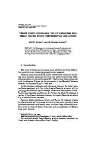
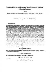
In the early years, experimental analyses were the only means available to Figure 1.1: Position of the MB in a fixed grid network

give an understanding of physical processes. However, with the advent of high

ce

speed digital computers, mathematical modelling and computer simulation

FGMs, where the Moving Boundary (MB) is often located between two

real process. This permits the simulation of the performance of new product

neighbouring grid points (Figure 1.1), break down when the boundary moves a

designs and the assessment of quality even before production, resulting in great

distance larger than a space increment during a time step. This restriction,

savings of time and money. Due to the wide range of applicability in engineering and science, in the last engineers and scientists alike. As analytical solutions are frequently impossible numerical analysis.

performed for extended times. The possibility of break down of the scheme is avoided in VSSMs, by using variable space elements (as shown in Figure 1.2).

/1

I

fe re

Finite Difference Methods (FDMs) are the most popular choice for numerical

size (memory) requirements and the cpu-time if computations are to be

e as

for most engineering and scientific applications, recourse must be made to

upon the velocity of the moving boundary, may considerably increase the array

e pl

two decades MBPs have drawn considerable attention from mathematicians,

l, fu

e us

are often the cheapest and fastest means to give a broad understanding of the

-----

solution of MBPs; however, in recent years, Finite Element Methods (FEMs)

require more cpu-time and are less suitable to vectorisation and parallel

Fixed Grid Methods (FGMs),

(ii)

Variable Space-Step Methods (VSSMs),

-

-

I

•

-1I

I I

I

I

------!-----:'----~:'-----I I

LIx

--- -- ,.'4__ I

I

.~ I

.. I

"

..'

,

./

~ I

ME

..

x

Figure 1.2: Position of the MB in a variable space grid network

ok

(iii) Variable Time-Step Methods (VTSMs).

-

bo

(i)

-

e th

Finite difference methods for solving MBPs can be classified into:

L1l.

'-:- -----'

-

e

computation than FDMs.

1

-' I

nc re

and Boundary Elements Methods (BEMs) have been introduced. The advantage of FEMs and BEMs is their ability to handle complex geometries; however, they

-

However, these methods present considerable computational difficulties (underflow and overflow) at the beginning of computation when the MB is too

4

Chapter I

Chapter I

Introduction

5

Introduction

If that the implicit methods, which are stable for any mesh size, are very

the enlargement of space elements which is a consequence of the displacement of the MB.

inaccurate when used with large time steps. The combination of the Virtual

u

yo

close to the fIxed boundaries; moreover, it loses accuracy at later times, due to

d fin

,L1x

I

- - - -

-.-,4-

,

I

I

I

- - ,- -

I

Due to the inaccuracy of the implicit fInite difference equations when the

I

,

.-

Fourier number is relatively large, a new numerical scheme which will be

-- - -- -I - - I

I

-

referred to as the Explicit Variable Time Step (EVTS) method is developed for

- - - - - -,- - - - - - - r - - - - - - r - - -

solving two-phase Stefan problems. Numerical results show that the EVTS

-,- -

I

I

-

-

-

-

I

I

-

-

-

-

-

-.- -

I

-

-

-

re

-

linear and non-linear partial differential equations.

- -

s

L1t

-

-

I

"

, -

- -

I

-- - -- -,- - - - - - -.- - - - - -

chapter also presents some recent advances in the fInite difference solution of

_,I

- - -

"

-

equations offers superior performance to that of the implicit equations. This

i th

- -- - - - ,- -

Sub-Interval Elimination Technique (VSIET) and the explicit finite difference

-

-.- -

-

I

I

,

I

,

I

I

I ,

I ,

I I

method out-performs the implicit methods in current use. This is the subject

ur

I

so

I

I

techniques which increase the accuracy of the methods presented in chapter 2.

VSSMs are avoided; this makes VTSMs a very attractive approach. However, VTSMs depends on the accuracy of recurrence formulae such as CrankNicolson and fully implicit equations, which are very inaccurate when time solve MBPs where the moving boundary has a relatively slow velocity. developed techniques for solving moving boundary problems. Chapter 2 reviews some of the well known numerical methods frequently used to solve moving

which will assist the reader who has a profound interest in the detailed account

fInite element method of Bonnerot and Jamet [7], and the finite difference method of Zerroukat and Chatwin [8] are reviewed and compared. In chapter 7, the different techniques illustrated in previous chapters are used on a practical application. This consists of the simulation of the heat flow during laser heat treatment of materials, where heating of solid, melting and resolidifIcation occur in a very short time.

Numerical results show good

agreement with experimental results.

ok

A comparative study of the fInite difference equations, which represents the basis of any finite difference scheme, is given in chapter 3. The study shows

interfaces appear and disappear during the process. Both the conservative

bo

of the mathematical and computational aspects of moving boundary or Stefan problems.

In chapter 6, multiple moving boundary problems are dealt with. A typical

problem is the collapse of a solid wall, where both mel ting and vaporisation

e th

essence of each approach. This chapter also contains important bibliographies

problem to illustrate their application.

e

boundary problems. The methods are briefly described in order to illustrate the

The chapter reviews and compares a number of

nc re

This book reviews and compares some of the well known and recently

the moving boundary.

available methods to solve this type of problem and uses the oxygen diffusion

fe re

step becomes relatively large; VTSMs may not be sufficiently accurate if used to

problem is different from the general moving boundary problems due to the absence, in its formulation, of an explicit expression containing the velocity of

e as

this approach is limited to one-dimensional problems only. As the accuracy of

This type of

e pl

rather than a space variable grid, the problems associated with FGMs and

Chapter 5 deals with implicit moving boundary problems.

l, fu

By using VTSMs, where a variable time grid network is adopted (Figure 1.3)

Furthermore, the more accurate fInite difference solutions

developed in chapter 3, are combined with algorithmic manipulation

e us

Figure 1.3: Position of the MB in a variable time grid network

ce

x

of chapter 4.

6

Chapter i

introduction

If u

yo

1.2. References

2.

M.M. Lame and B.P.E. Clapeyron,Ann. Chem. Phys. 47, 250-256 (1831). J. Stefan, Sber. Akad. Wiss. Wien. 98,473-484 (1889).

d fin

l.

J. Stefan, Ann. Chem. Phys. 42,269-286 (1891).

4.

J. Crank, Free and moving boundary problems, Clarendon Press, Oxford (1984).

s

i th

3.

RM. Furzeland, J. Inst. Math. Appl. 26, 411-429 (1980).

6.

E. Magenes (ed.), Free boundary Problems vols. I and II, Instituto

so

re

5.

Nazionale di Alta Matematica Francescon Severi, Rome (1980). 8.

M. Zerroukat and C.R Chatwin, J. Comput. Phys., (in press).

ce

R Bonnerot and P. Jamet, J. Comput. Phys. 41, 357-378 (1981).

Numerical Methods for Moving Boundary Problems

2

ur

7.

l, fu

e us Summary

e pl

e as

Chapter 2 reviews some of the well known numerical methods frequently used to solve moving boundary problems. The methods are briefly described in order to illustrate the essence of each approach.

This chapter also contains an

fe re

important bibliography which will assist any reader who has a profound interest in the topic.

e

nc re e th ok

bo

8

Chapter 2

Numerical methods for MBPs

Chapter 2


9

If Material thickness Specific heat

K

Thermal conductivity

Latent heat of fusion/unit volume

methods.

2.2. The heat balance integral method (Goodman)

L\t

Time step

L\x

Space element

ib

Subscripts Space step index Interface node index

By integrating the one-dimensional heat flow equation with respect to the

i th

Heat transfer coefficient Enthalpy

Material density

A.

d fin

h H

are often used as a reference standard against which to validate the numerical

p

u

a c

yo

Nomenclature

Position of the interface Latent heat offusion =IJp

r

Fourier number

j

Time step index

t

Time variable Temperature

m s

Melting

T

produced an integral equation which expresses the overall heat balance of the

re

Superscript

a

Diffusivity

Iteration index

conditions, e.g. a polynomial relationship. (ii)

However, with the onset of the computer revolution, MBPs have been the focus large number of numerical schemes have been developed. It is not feasible to

change boundary and the time dependence of the temperature distribution.

e as

of intensive research during the seventies and eighties, during which time a

(iii) Solve the integral equation to obtain the motion of the phase

e pl

Research on Moving Boundary Problems (MBPs) started as early as 1831.

assumed temperature distribution to obtain the heat balance integral.

l, fu

2.1. Introduction

Integrate the heat flow equation with respect to the space variable over the appropriate interval and substitute the

e us

Liquid

Space variable

ce

Temperature at the interface

on the space variable which is consistent with the boundary

ur

Tb

system. The successive steps in Goodman's method are: (i) Assume a particular form for the dependence of the temperature

so

Solid

x

k

space variable x, and inserting the boundary conditions, Goodman [15]

s

M L

2.2.1. Heat balance method for the single-phase ice melting problem The heat balance method can be conveniently illustrated by solving the

reports [1-14] are available which contain up to date accounts of the

single-phase melting-ice problem in one space dimension as defined by the

mathematical developments in this field, they illustrate wide ranging

following equations using dimensionless variables.

Finite difference methods have been used extensively for solving moving

methods compute, at each time step, the position of the moving boundary as well as the temperature at each grid point of the space-time domain. Before

, t>O

T(x,t) T(x,t)

=

(2.1)

1 , x=O , t > 0

(2.2)

, x>O , t = 0

(2.3)

= 0

M(O)

= 0

ok

Neumann's methods [16] are illustrated; these are analytical methods which

, O:=:;x:=:;M(t)

bo

presenting the numerical techniques, the well known Goodman's [15] and

at =

a 2T ax 2

e th

methods which can be used to solve these problems are reviewed. These

dT

e

boundary problems. In this chapter, some of the well known numerical

nc re

applications in physics, biology and engineering.

fe re

review all of them in this chapter; however, many surveys and conference

(2.4)

10

Chapter 2 Numerical methods for MBPs


11

If =0

yo

T(x,t)

x

,

= M(t) , t > 0

u = dM dt

, x

= M(t)

, t>

left side of (2.7) gives

°

(2.6)

d fin

- aT ax

Substitution of(2.8) incorporating get) and rp(t) from (2.11), and integrating the

(2.5)

dM -1( 1+.../3 )dM = ---(g -2rpM) 6 dt dt

(2.12)

i th

where T, t, x and M refer to temperature, time, spatial location and the position of the moving boundary, respectively.

Further elimination of

g and

rp from (2.12) gives

s

=

°to x = MCt), gives

= [3..Jt

(2.14)

By substitution of (2.14) and (2.11) into (2.8), the temperature distribution which represents the solution of the problem, defined by (2.1) to (2.6), is readily

obtained.

2.2.2. Heat balance method for two-phase melting of a finite slab

e as

dx

(2.13)

e pl

ax

(2.9)

x = M(t)

M(t)

l, fu

(2.8)

which satisfies (2.5). It is convenient to modify the condition (2.6) to the form

2 ( ar)2 = d ; ,

[3 = ,I 7 +.../3

from which it follows that

e us

Assuming a temperature distribution in the water phase given by

T(x,t) = W){x - M(t)} + rp(t){x - M(t)}2

12(3- .../3)

where

(2.7)

ce

fT(X t) dx = _(dM + aT(O,t») dt' dt ax o

M dM = 6( 3 - .../3) _ 1 2 dt 7+.../3 -"2[3

ur

!!:...

so

M(t)

re

Integration of (2.1) with respect to x, from x

The heat balance method was applied to solve the melting of a finite slab of

by using the standard formula

=

The problem is described by the following equations

° , x = M(t)

(2.10)

nc re

dT _ aT dM + ar dt at

de - ax

fe re

thickness a initially at a uniform temperature that is below the melting point.

'

°x $;

$;

M(t)

(2.15)

a2 ax

,

M(t)

$;

x

(2.16)

ar/- a _/ dt

ax

ar

at

(2.11)

/ ar/ ax -Ks ar ax

s

a

, x = M(t)

ok

=A dM) dt T/(x,t) = Ts(x,t) = T b

K

$;

bo

M(t)

gM+1 rp =---,;j2

e th

s a - T- s -= s 2

x = M(t), so that the substitution into (2.9) yields

g = 1-.../3

e

to replace (dM / dt) in (2.6). Taking into consideration that T(O,t) = 1, (2.8) gives: 1 = -gM + rpM 2 and on differentiation, aT / ax = g, a 2T / 2 = 2rp at

2

a T/2 ax

(2.17)

Chapter 2

12

13



If yo

~l(t), ~s(t),

heat capacity, temperature at the moving boundary and latent heat of fusion

f{J1(t) and f{Js(t) are determined so that the temperature distributions, (2.22) and (2.23), satisfy the boundary conditions. For

per unit volume, respectively. The subscripts land s denote liquid phase and

example, with the following boundary conditions

where ex=KI(pc), K, p, C, T b and

A. are diffusivity,

The parameters

thermal conductivity, density,

u

d fin

solid phase respectively. The solution of the problem during the pre-melting

-Kl ( arl )

stage is not presented since standard solutions are readily available in [16].

i th

ax

Goodman and Shea [17] have also solved for this stage by the heat balance

s

method.

=F

x=O

re

from x=o to x=M(t) and (2.16) from x=M(t) to x=a to obtain the integral equations

ax

M(t)

dM }=!!:...fa Tsdx+Tb dt dt

(2.19)

M

ax) and (ar s I ax), at x = M(t),

from (2.18) and (2.19) and

making use of (2.17), yields

al dt

, Tb

=0

(2.24)

= F

(2.25)

as dt

_(a - M)2 dO

s _

°

3as

(2.26)

(2.27)

s

dt

Equation (2.25) is obtained by substitution of (2.24) into (2.20). The evaluation of

e pl

Elimination of (arl I

a

l, fu

ax

=0

01 = M2(~ __1_dOI) 2Kl 3al &

e us

as{(aTS ) _(ars)

(2.18)

ce

f

- (arl - )} = Mfarl - d x =d- M T l dx-Tb -dM ax 0 ax dt dt o 0

dt

ur

M(t)

x=a

-A. dM + Kl dOL + K s dO.

so

ax

, Ks(O:XS )

Goodman and Shea [17J arrive at the following differential equations

Following the three stages (i) to (iii), defined in section 2.2, (2.15) is integrated

al {( -arl )

= const.

~l(t)

and f{J1(t) using the conditions (2.24) and (2.18), and using the first

K s Tb _ K l T b _ A.) dM + K l dOL + K s dOs = Ks(aTs ) _ K ( aTI ) ( as al dt al dt as dt ax x=a l ax x=O

(2.20)

e as

integral of (2.21),gives (2.26). Equation (2.27) is derived by first evaluating

~.(t)

and f{Js (t) using (2.24) and (2.19) and finally using the second of (2.21).

fe re

To solve the equations (2.25) to (2.27), the following initial conditions are where

needed

Os = f Ts(x,t) dx

(2.21)

M

M(tm)

=0

-F a 2

°s(tm) = 3K s

Ol(tm) = 0

(2.28)

e

° 1 = f T/(x,t) dx o

a

nc re

M

e th

Os (t m ) of (2.28) is obtained by integration with respect to x, from x

Suitable temperature distributions are then chosen to be

= 0 to x = a,

(2.22)

Ts(x,t) = T b + ~.(t){ x - M(t)} + f{Js(t){ x - M(t)} 2

(2.23)

Ts(x,t m) = -aF {~(2-~)} 2K. a a

ok

Tl(x,t) = T b + ~1(t){X - M(t)} + f{J1(t){X - M(t)}2

bo

of the temperature distribution Ts(x,t m ) at the time when melting starts which is given by Goodman and Shea [17J as

(2.29)


Chapter 2

If

14

aT. aT= dM l K -KlpL -


• ax

yo

Goodman and Shea obtained the solution of (2.25) to (2.27) by lengthy

ax

u

T.(x,t) = Tl(x,t)

(2.27), can be obtained easily using a standard method such as Runge-Kutta.

x= M( t )

(2.32)

= M(t)

(2.33)

dt'

mathematical manipulations. As an alternative method, solution of (2.25) to

=T b

,

x

15

d fin

Many authors [18-24] have applied the heat balance method to different where L is the latent heat of fusion.

problems, as well as studied ways of improving and easing the mathematical

i th

analysis. The mathematical manipulations required for the heat balance

I - The region x> 0 is initially liquid at a constant temperature To, with the

method, for anything other than relatively simple problems, can be very lengthy

s

surface x = 0 maintained at zero temperature for t > 0 (Figure 2.1).

and complicated. Furthermore, the choice of a satisfactory approximation to

re

the temperature distribution is a major difficulty with the method. For

so

example, the use of a high order polynomial for the temperature profile makes

x M(t)

(2.31)

,

00

x=O

= Aerf[ 2(a:t)1J2 ]

Tl(x,t)

=To -

Berfc[

2(al~)112 ]

(2.34) (2.35)

(2.36)

(2.37)

where A and B are constants which satisfy (2.30)&(2.35) and (2.31)&(2.34)

bo

2 l a la-T-l aT_0 2

T.(x,t)

e th

•

2

,

-1

The solution of problem I can be written [16J as

e

aT. _ a (iT.

when x

To

T.(x,t)=O

nc re

techniques, since it is possible to obtain an analytical solution. In general, the

4

fe re

The method is illustrated for a number of simple heat transfer cases [16J.

at

The equations to be solved are (2.30), (2.31), (2.32), (2.33) with the following additional boundary conditions

e pl

including that of the melting boundary, at successive times.

at

l, fu

than subdividing the space variable. The solution of a system of differential

respectively. Equation (2.33) requires that

ok

16

17



If yo

For the special case in which the liquid is initially at its melting point, i.e.

Aerf[ M(t)112 ] = To - Berfc[ M(t)112 ] = T b 2(as t) 2(a/ t)

To

(2.38)

= T b , (2.41) reduces to

u

d fin

i th

M(t) = 2w(as t)1I2

wexp(aherf(w) =

..Jt, that is

To satisfy (2.38) for any value of t, M must be proportional to

s

where w is a real constant to be determined from the condition (2.32). Making use of(2.36), (2.37) and (2.39) wmust be the solution of

Assume

re

r

••pC-m ) -

)112] -

KsTb{a; erfc w( :;

csT b

(2.41)

x = 0 ~:: .... ;::::~i:;l: :~:~j~~:: :;;:~:::~y~: .':-:;:~;;

.,

x> 0

!C"";'

I. j

LlqUld

_.,.__ .,.' T b, as shown in

solid (Figure 2.4).

s

:::~TK~'t,

"

Solid

T-

-0

'fffffr'

ti::;:::::::::~:~ ;: : :;.:.:.:.:.: ~::;.:.:.:.:.:.:.:.:.:.:.:r::::::::~::::;:::::::::;:::;:;::=;:::;::;:::.

ce

x>O

ur

so

::oJr~i!.T=T'>Tb

l, fu

t> 0

(2.51)

KsTb{a; exp( -alm / as)

mL...{;

Kl{a;(To -Tb)erfc[m(al / a s )1I2] = cl(To -Tb )

(2.52)

2(as~t)1/2])

T"l(X,t)=B+cerf[ 2(a:t)1/2]

fe re

2

T S1 (x,t) = A[ 1 + erf[

e as

where mis the root of exp(-m 2) erf(m)

The solution of the problem can be written as

e pl

M(t) = 2m(al t)1/2

nc re

Tl(x,t) = To -nerfc[

The temperature distributions in both regions are given by

(2.53)

(2.56)

(2.57)

The temperature continuity

relations at x=O require that

A=B

, Ks1A.,Ja;; = K"lCF::

bo

- T b) erf[ 2(alxt) 112] Tl(x,t) = To - (To erf(m)

0 as x ~ - 0 0 ,

e th

Tb erfC[ x ] erfc[ meal / a s )1I2] 2(as t)1I2

~

2(al~)IJ2 ]

(2.55)

e

Equation (2.55) makes T S1 (x,t)

Ts(x,t) =

)~'~~;i~~,i!~][~~:i~~]i~i!!liii!ii~~~!!j~l::Ch

Figure 2.4: Case IV

e us

Similarly to the previous cases, the interface is written as

x - M(t

t=O

11

Figure 2.3: Case III

x < O ~KS1,cS1 x=O~n~~~~ _ ~E2!i
X 0 initially at T b2 and x =0 at zero temperature, (2.41)

so

different regions can be written as

T~

(2.60), bearing in mind that Cl, in (2.41) and (2.60), is the value given by (2.65).

After determination of w from (2.60), the temperature distributions for the

T (x t)-

(2.65)

T~ s T s Tb,.

l;.. ~,~,~,~,~,~,~ ....,....,,..,.....".,....." ... '~ ... ~,~ ... :'~,~ ':'~ ':,.

:'~/~":":/>:' Phase 2

>.:':':':':':':':':

1

e

r. O. It is assumed that the material has two

the latent heat L and the specific heat Cl' of the homogenous liquid

transformation temperatures T bl and T~, V>

ok

bo

temperature T bl and T~. Assuming that the latent heat in the mushy region is liberated linearly with temperature, this effect can be taken into

T~

>Tbt >0, at which the latent



22

23

If ~

VII - The effect of density change

yo

heats L l and

are liberated respectively. The subscripts 1,2 and 3 are used to

u

denote the regions 1 (where the temperature varies from 0 to T bl ), 2 (T b1 , Tb-z)

When the change in density of the material, due to the phase changes, is

interfaces: x

= Ml(t)

d fin

and 3 (Tb.z' V), respectively (Figure 2.5). Consequently there will be two moving separating phases 1 and 2, and x

= M2(t)

taken into account, in a similar manner to (2.36), the temperature in the solid region can be written as

which separates

phases 2 and 3. Following the same procedure as for previous cases, the

i th

moving boundaries can be written as

s

X T.(x,t) = Aerf[ 2(a t) 112 ] (2.68)

Since the liquid and solid have different densities, then, when the interface moves a distance dM, the liquid moves with a velocity ur given by

so

re

Ml(t) = 2wl(aIt)1I2

where Wl and W2 are the solutions of the following system of equations

ur K 2..j(i;(Tb-z -TbJexp(-wr a l/a 2}

-

Cl

-

C2

ax

different regions can be written as

PIal

dt

(2.71)

ax

al at

x + w(Ps - Pl){a;] 2(al t)1I2 Pl{a;

(2.77) requires that Tl(x,t) ~ To as x ~

nc re

er~b~l) (erf[ 2(a;t)1I2 ]J

fe re

Tl(x,t) = To - Berfc[

T I(X,t) =

_l)dM dt

(2.75)

(2.76)

If M = 2w(as t)1I2, (2.76) is satisfied by

e as

Having determined iteratively wI and W2' the temperature distribution in the

=_(Ps PI

a2~1 + (P. - PI) dM arl _ -.!. arl = 0

e pl

K 2.,J'a; erf[ W2{ a2/(3)1I2]

erf(Wl) - erf[WI( al/(2)l/2]

r

The heat equation in the moving liquid is then written as

l, fu

K3~(To-Tb2}exp[-w~(a2/a3)]_ w2L2~ (2.70)

(Tb-z - T bl }exp(-w~)

U

(2.69)

e us

{erf(W2)-erfc[Wl(al/a2)1I2]}Kl~

_ wlLl~

ce

T bl exp(-w~) erf(w l )

(2.74)

s

M 2(t) = 2w2(a2 0 112

00.

(2.77)

The temperature continuity at the

moving boundary x=M(t), requires that

= To -

(2.73)

(2.78)

Following the same procedure as case I, and making use of (2.78), co is determined from the solution of

ok

(To-Tb-z) erfc[--X--=-=-] erfc[ W2(a2 / (3)1I2] 2(a3 0 1l2

Aerf(w) = To - Berfc[wPS{a;] = T b PI {a;

bo

T 3(x,t)

(2.72)

e th

(Tb-z - T bl )erf[ x/2(a2 0 112 ] + T bl erf(W2) - Tb-z erf[ WI( ad(2)1I2] [112] erf(w2)-erf wl(ada2)

e

T 2 (x,t) =



24

25

If yo

The variation of the position of the moving boundary is given by (2.79)

u

exp(-w 2 ) erf(w)

d fin i th

2.4. Fixed grid finite difference methods

Pj+1

){ Pj Pj + 1 } = Pj - ( .t t.t L1x2 Pj + 1 Tib-l,j --p;-Tib,j

(2.82)

Various finite difference schemes have been proposed for approximating

s re

both the boundary conditions and the partial differential equation at the neighbouring grid points. For instance, Murray and Landis [28] used a fixed

Using finite difference techniques, the heat flow equation is approximated by

grid network. In particular, in the sub-space containing the fusion front at any

temperature Ti,j' at xi = iL1x and time t j = jt.t on a fixed grid in the (x,t) plane. At any time t j = jt.t, the phase change boundary will usually be located

time, they introduce two fictitious temperatures, one obtained by quadratic extrapolation from temperatures in the solid region and the other from

between two neighbouring grid points; for example: between ibL1x and

temperatures in the liquid region. The fusion temperature and the current

ur

so

finite difference replacements for the derivatives in order to compute values of

ce

+ 1)L1x, as shown in Figure 2.6.

(2.81). For the motion of the fusion front, an expression analogous to (2.82) is used based on the Taylor extrapolation formula. Furzeland [29] suggested using an approximation for (iJT / be eliminated by use of(2.80).

ax)

on the MB with a fictitious temperature to

e as

ib +2

ib + 1

compute temperatures near the interface instead of using special formulae like

e pl

9~H ib

are then substituted into the standard approximation, such as (2.80), to

l, fu

x=M(t)

ib -1

position of the interface are incorporated in the fictitious temperatures, which

e us

(ib

The advantages of implicit finite difference equations have been investigated

Figure 2.6: Location of the moving boundary in a fixed grid

by Ehrlich [30], Koh et al. [31], Saitoh [32], and Bonnerot and Jamet [33]. For

fe re

example Meyer [34] obtained a second order approximation for the movement of The numerical solution of the single-phase problem, defined by equations (2.1)

the MB by using a three-point backward formula. Ciment and Guenther [35]

to (2.6), provides a simple example and proceeds as follows: the temperature

employed a method of spatial mesh refinement on both sides of the MB,

nc re

T i,j+1' as a function of temperatures of the previous step, is given by

previously analysed by Ciment and Sweet [36]. They also incorporated the idea used earlier by Douglas and Gallie [37], of adjusting the time step so that the

i=0,ib -1

(2.80)

MB coincides with one of the refined mesh points. Huber [38] used an implicit

e

T·I,J+ . 1 = T·I,J. +(~){T' L1x 2 1- l.J' -2T·I,J. +T,1+ 1,J,}

J

Lazaridis [40 I used explicit finite difference approximations on a fixed grid to solve two-phase solidification problems in both two and three space dimensions.

(2.81)

ok

'-~T'.} P' "b,J

2t.t){ T-"b,J'+1 = T ib, J' + ( -L1x 2 -11 T,"b- 1,J Pj+

simplified by Rubinstein [4J and Fasano and Primicerio [39].

bo

By using three-point Lagrange interpolation [27], instead of (2.80), the temperature at x = ibL1x is calculated using

e th

scheme for approximating the heat flow equation in each time step, but he tracked the MB explicitly using the Stefan condition; this approach was later

He wrote the heat balance condition on the MB in Patel's expressions and

26



Chapter 2

If

iII') = (at

yo

developed numerical schemes based on an auxiliary set of differential equations, which express the fact that the ME is an isotherm. These auxiliary

i

Xi

M(t)

u

(iII') a dt at + ax 2

dM

T

27

(2.85)

2

forms are compatible with Patel's expressions in enabling the boundary

d fin

movement to be computed in the direction of the coordinate axes, rather than

The position of the moving boundary M(t) is updated at each time step by

along the normal to itself. Standard finite difference approximations to the heat

using, for example, a suitable finite difference form of the boundary condition

-iII' /ax) on

(dM / dt

Westwater [41J to convection problems and by Tien and Churchill [42] to

s

i th

flow equation were used at grid points far enough from the ME. Near the boundary, formulae for unequal intervals were incorporated into the auxiliary equations. To avoid loss of accuracy associated with singularities, which can

=

X

= M(t).

The method was extended by Heitz and

cylindrical coordinates. Crank and Gupta [43J avoided the complications due to the unequal grid size

profiles were used. The mathematical manipulations are very lengthy and

near the MB by moving the whole uniform grid system with the velocity of the

complex indeed.

ME. They described two methods of obtaining the interpolated values of

ur

so

re

arise when the MB is too near a grid point, localised quadratic temperature

temperature at the new grid points, to be used for the next time step, based on

ce

2.5. Variable space grid finite difference methods

cubic splines or polynomials. Later Gupta [44,45] avoided the interpolations by

e us

using a Taylor expansion of space and time variables and derived an equation

Several techniques of modifying the grid have been proposed, all with the

which can be seen as a particular case of (2.85).

aim of avoiding the increased complication and the loss of accuracy associated

interval, L1x = M(t) / q, is different for each time step. The ME is always on the Xi

grid line. They differentiated partially with respect to x. Thus, for the line = iL1x the heat equation becomes

decided to determine,

as part of the

solution, a variable time step such that the MB always coincides with a grid

line in space. They used the fully implicit finite difference equation; this leads

(2.83)

fe re

to a system oflinear equations to be solved at each time step.

(~} =(~)J:}+(~)x

Gupta and Kumar [46] formulated the same set of finite difference equations as Douglas and GaBie but they used the interface condition to update the time

Xi

moved according to

the expression

nc re

Murray and Landis assumed that a general grid point at

Douglas and GaBie [37] instead of using a fixed time step and searching for

the position of the moving boundary,

e as

qth

2.6. Variable time step grid finite difference methods

e pl

Landis [28] kept the number of space intervals between a fixed and moving boundary constant, for example equal to q, for all time. Consequently the space

l, fu

with unequal intervals near the MB in the fixed grid network. Murray and

step .1t. They thus avoided the instability which develops as the depth of the ME increases; the instability is generated as the time step enters an infinite loop

e

because it becomes very sensitive to rounding errors. Goodling and Khader [47J

dt

M(t) dt

(2.84)

e th

dx i =~dM

incorporated the finite difference form of the MB condition into the system of equations to be solved. The system is solved for an arbitrary value of the

The one-dimensional heat equation becomes

bo

temperature of the node neighbouring the MB, which is then updated from the boundary condition. Gupta and Kumar [48] found this latter method fails to

ok

converge as the computation progresses in time, because it is too sensitive to a small change in temperature. Gupta and Kumar's results are in good

28


29


If yo

agreement with those obtained by using the the integral method of Goodman

Suppose the moving boundary is moving from the nodal point (ib,j) to

and other variable time step methods. Gupta and Kumar [49] also adapted the

u

(ib + 1,j + 1), then the problem is to compute: the time step L1t j necessary for the

method of Douglas and Gallie to solve the oxygen diffusion problem (implicit

d fin

ME to move a single spatial step, and the temperature distribution at the time

moving boundary problems). Their results compare favourably with those

tj+l

obtained by Hansen and Hougaard [50] and by Dahmardah and Mayers [51].

(i.e. Ti,j+l' i

= O,N) from

(see Figure 2.7).

i th

To illustrate the variable time-step methods, consider the following problem,

= a aT

,

iJx2

0:5 x :5 M(t)

ax

t~O

M(t):5x:51,

,

x

= M(t)

t>

(2.89)

a

=a

(2.90)

ib -1

central finite difference, gives

(2.92)

Rearrangement of (2.92) gives

= Ti,j

,

i=1,i b

(2.93)

e

i=1,2,

N

(2.91)

where rJ = a L1t j / Llx 2 is the Fourier number.

e th

,

m=O

In order to determine L1tj , both sides of(2.86) are integrated with respect to x, from x = a to x = M(t), making use of(2.87). This gives M(t)

:t

]

ok

to x = (m+ 1)Llx.

bo

where L1tm denotes the time interval in which the boundary moves from

= mLlx

2Ti,j+l + Ti+l,j+l] Llx 2

nc re

j-l

x

= a(Ti-1,j+l -

fe re

Tj,j+l - Ti,j L1t.)

(1+2rj)Ti ,j+l-rj(Ti _l,j+l+Ti+l,j+l)

t j = LL1t m

ib +2

ib + 1

ib

2.6.1. The Extended Douglas and Gallie's (EDG) method

Llx during the time interval. Any point (Xi,t j ) in the space-time domain is

given by the coordinates

,

I

~-----

_________ I

Figure 2.7: Movement of the MB x = M(t) in a variable lime step grid network

e as

at each time stepj, is chosen such that the boundary moves a distance

xi=iLlx

v

,

Let Ti,j be the temperature at the coordinates xi,t j . Replacing the left side of (2.86) by a backward finite difference at the point (Xi,t j ) and the right side by a

The region 0:5 x:5 1 is divided into N sections of length Llx = 1/ N. The time .t1t j'

I

)

(2.88)

where h is a convective heat transfer coefficient and IJI is a real constant.

step

I

e pl

M(O)

,

I I I

Phase 2

.t1x

(2.87)

a

~---------r-----

l, fu

aT

dM dt

,

t >

'

.t1t j

(2.86)

e us

=1

=a ,

a

ce

T(x,t)

, x

t>

ur

aT ;;; = hT + IJI

,

I'

Phase I

so

at

1

)+1

I

re

2

aT

x=M(t)

s

in dimensionless variables,

a known temperature distribution at the time tj

IT(X,t)dx-(a+1)M(t) =-a(hT(O,t)-IJI) [

(2.94)

30


31


If yo

Further integration of (2.94) with respect to t , and making use of (2.90), gives

u

Similarly, the (k+1)th iteration for calculating ,1tj can be written from (2.97)

a'lfl + ah T(O,t)dt

= (a + l)M -

o

f

d fin

f

as

M

t

T(x,t)dx

(2.95)

k 1

= t j + 1 , gives

re b

+1) T i +l,j+1

a( h + vfl'O,j+1)

e as

matches with the one obtained by satisfying the boundary conditions (2.87) and (2.89). The special case of ib = 1 is discussed in section 2.6.3.

Goodling and Khader [47] used the same set of simultaneous equations, (2.98) and (2.99), to determine the temperatures at time t j + 1 at the k th iteration. The boundary condition (2.89) is replaced by the following finite difference equation

e pl

It should be noted that in (2.96), the finite difference replacement of the integrals have been made such that the value of ,1tj , obtained from (2.97),

2.6.2. Goodling and Khader's (GK) method

l, fu

(2.97)

k k _&1 (T 'b+l,j+1 _T'b,J+l . ) = &-

,1t~

accuracy in ,1tj is achieved. The k th iteration for solving the system of (ib + 1)

,1t k J

linear equations is

(2.101)

J

nc re

giving

fe re

By choosing a suitable estimate of ,1tj , the temperature at any grid point is computed from (2.93) and the estimated value of ,1tj is subsequently reevaluated from (2.97). This iterative process is repeated until the desired

(2.100)

a new temperature distribution T i: j + 1 , i = 0, ib . This process is repeated until the desired accuracy in ,1tj is achieved.

e us

,1t j

i

.=1

k)

the new estimate of ,1tJ from (2.100). ,1tJ is substituted in (2.98) and (2.99) to give

ce

Mter manipulation, (2.96) becomes

t;

(

+1)

Choosing ,1tJ equal to ,1tj _1 which is already known, T~j+1' i = O,ib are determined from (2.98) and (2.99). These values are in turn used to determine

(2.96)

ur

so

a'lflj+1 + ah L(To,p ,1tp_1) = (a + 1)(j + l),1x - & LTi+l,j+1 p~l i=l

j

i

~ Ti.1,j+1

a h + vfl'O,j+1

J

ib+1

(a + 1)(j + 1)& - alpt j + ah ~ (To,p ,1tp_1) - &

p=l

,1t· + =

s

j+1

b

j

(a+ l)(j + 1)& - aljltj + ahL(To,p ,1tp_1) - &

i th

The finite difference replacement of (2.95), when t

f

j

0

&2 (2.102)

k

1-Tib ,j+1

e

rj

(Ti~l,j+1 + Tt'tl,j+1) = Ti,j

= ljI&

= a ,1tj / &2 and T i:+l,j+1 = 1 from (2.88) for all k.

(2.98)

(2.99)

The method suggests that after choosing a value of Ttj+1' ,1tJ is recalculated from (2.102). The value of ,1tJ is used to calculate T~j+1' i = O,ib Using (2.98). Equation (2.99) is then used to test the accuracy of the selected value of Ttj+1' If (2.99) is not satisfied, T ib ,j+1 is estimated again and a new ,1tj is obtained from (2.102), which in turn is used to calculate new values of Ti.J+l , i

= O,ib .

ok

where rj

= 1,ib

bo

Ttj+1 - (1 + h&)Ti,j+1

i

e th

(1 + 2rj)T!~j+1 -

This process is repeated until (2.99) is satisfied within a

33



32

If yo

T ib ,j+1

The first time step

was selected is not explained

is calculated by combining both the boundary

11to

condition (2.87) and the interface condition (2.89). The finite difference of (2.87)

u

specified error. However, the way in which in detail by the authors.

Gupta and Kumar [48], in a comparative study of numerical methods for

d fin

gives

moving boundary problems, tackle this point. They tried taking T?b. )'+1 equal to Tib-l,j as a suitable estimate; then kept increasing it by small increments until

1 L1x'

- ( T11 -To

s

i th

a change of sign in the error in (2.99) was detected; then T ib ,j+1 was interpolated either by the method of chords or the bisection method. They found

(2.105)

•1) = hTo•1+ lfI

and the finite difference of (2.89) gives

re

that this procedure does not always work. In the problem they solved [48J the procedure fails after a number of time-steps; the method of solving (2.98)

so

L1x

11tJ

from the following

+ (11tj-1 -

11tj-2) + e

process is repeated until a change of sign in the error occurs; then the value of

L1x( 1 + hL1x )

(2.107)

(h + lfI)

In sections 2.6.1, 2.6.2 and 2.6.3 the computational procedure, of passing from one time step to another, for each method is explained. At the beginning of computation where the moving boundary is moving from x

is interpolated by the method of bisection.

e as

11tj

= 1, the following is obtained

e pl

is incremented by approximately 0.2% and the

11tj

Tl,l

11to =

l, fu

where eis small. Ttj+1 is calculated from (2.100); values of T~j+1' i = O,ib are then determined from (2.98); (2.99) is checked to ensure that it is within the specified error; if not,

node (1,1) and therefore

(2.103)

e us

11tJ = 11tj-1

Combining (2.105), (2.106) and remembering that the moving boundary is at the

ce

they estimated

T ib ,j+1'

ur

Therefore, they adopted the following approach: instead of estimating

(2.106)

--.!..-(TO,l -Tl,l) = 11t L1x o

becomes unstable and the error in (2.99) behaves in an irregular manner.

any of the EDG, GK and MVTS methods, the time step

=0 to x = L1x,

11to

using

is calculated from

(2.107) without iteration and the temperature at x = 0 is calculated using

2.6.3. The Modified. Variable Time Step (MVTS) method

fe re

either (2.105) or (2.106). In this method [48) the same set of simultaneous equations, (2.98) and (2.99), written as

2.7. The enthalpy fonnulation teclmiques

nc re

are to be solved as in the EDG and GK methods. The interface condition (2.89) is

These techniques are based on the relationships which exist between the (2.104)

e

different thermodynamic properties of the material such as enthalpy, heat capacity and latent heat of fusion. These methods are strictly limited to melting

e th

11tY1=~ I-T~ .

'b.)+l

(freezing) problems, where the enthalpy formulation automatically satisfies the

= O,ib

equal to

11tj _1

initially, the temperature distribution

is obtained using (2.98) and (2.99). Using the value of

T?b· )'+1

in

(2.104) the new estimate 11t} is obtained. The process is repeated until the specified error in 11tj is reached.

jump in heat flux across an isothermal moving boundary. For instance, these methods cannot be used for implicit moving boundary problems, where the moving boundary is present due to physical phenomena other than a phase change [52J.

ok

T,O)'+l ,i •

11tJ

bo

Choosing

34

Chapter 2

35



If yo

,~ ~{:."

u

2.7.1. Post-iterative (Isothermal)

Solid region Mushy region Liquid region

TT 2

(2.109)

d fin

This is probably the simplest method r53,54]. For each node the usual finite where

C + (L/LlT);

change is occurring the temperature is set back to the temperature of transition

T 1 and T 2 are the temperatures at the lower and the higher ends of the mushy region, respectively. The apparent capacities are

and the equivalent energy is added to an enthalpy budget for that node. Once the

calculated using the temperatures at the nodes, and the resulting finite

difference or finite element equations are used. For the nodes where the phase

s

i th

budget is equal to the latent heat for the volume associated with that node, the

Cmu

=

difference or finite element equations are based on these apparent capacities.

re

temperature is allowed to vary according to the Fourier conduction equation.

so

2.7.4. Enthalpy method

ur

2.7.2. Post-iterative (Mushy)

In the enthalpy method [60 - 64], the heat conduction equation is written as

ce

This is similar to the isothermal case except that a mushy range (see appendix A) is also taken into consideration [55,56]. The latent heat is released

e us

at

over a temperature range, and is assumed to be a function of temperature

(generally linear) in that range. The procedure is as in 2.7.1 except that the

l, fu

temperature will be set to

= T 2 -( ~)LlT

(2.108)

are: heat in enthalpy budget, latent heat of fusion and difference of temperature as finite element formulations,can be used for the partial differential equations.

H(T)= cT + L(T-T 1 }

JcT

T 2 -T 1

Tl~T~T2

T > T2

Solid region Mushy region

(2.111)

Liquid region

fe re

of the mushy range. Again both implicit and explicit finite difference, as well

T0

(3.82)

Assuming the following thermal dependencies

without loss of accuracy or stability. It consists of automatic generation of Virtual Sub-time-Steps (VSSs), which are progressively eliminated as the

O:S x :S 1 ,

,

e th

The VSIET can also be used for non-linear problems [26]; it permits the use of large time steps for any of the explicit equations (equation (3.68) or (3.74»

temperature distribution Ti,j' i

ax

nc re

2Ki _l,jKi ,j K i- 1J2 ,j = K i- 1,j + Ki,j

()T =-a(K(T)()T)

C(T)-

fe re

separating the grid points. K i - 1J2 ,j and K i +1J2 ,j can also be evaluated using the

e as

In equation (3.75), a linear interpolation is used for the thermal conductivity

(3.83)

70

Chapter 3

Computational performance of FDMs

Chapter 3

71


If

and choosing the following boundary conditions

yo

similar accuracy; however, (3.69) requires fewer operations.

u

ry(x) ::: aexp( -c x)

times more accurate than the classical ones. Equations (3.69) and (3.71) achieve

!P(t) ::: aexp(bt)

,

rp(t) ::: a exp(bt - c)

(3.84)

d fin

t he following is an exact solution for equations (3.79) to (3.82)

Table 3.7: Comparison of percentage deviations (X10 2) at the centre of the slab

i th

T(x,t) ::: aexp(bt - c x)

time

(3.85)

s so

re

where a, b, c and d are real constants.

The problem defined by (3.79) to (3.82) is solved using the classical equations

ur

(i.e. (3.74)&(3.75)), the equation of Patankar (i.e. (3.74)&(3.76)) and the finite

ce

difference equations due to Zerroukat and Chatwin (i.e. (3.68)&(3.69) and (3.68)&(3.71)). The VSIET is incorporated with all the equations. For accuracy

e us

assessment, the numerical results are compared with the analytical solution and expressed in terms of percentage deviations defined as PD. . ::: 100 x (Ti •j ) Nu -

".J

(Ti •j ) An () T· . '.J An

(3.86)

that both the classical finite difference equations under-estimate the solution; whereas, (3.68)&(3.71) give an over-estimated solution; however, the numerical

-D.l788 -D.2261 -D.2520 -D.2588 -D.2647 -D.2697 -D.25 17 -D.24 19 -D.2255 -D.2101

Analytic

(3.68)&(3.69) PDN /2,j

T(~,tJ)

+0.03765 +0.03617 +0.01738 -D.00835 -D.00802 -D.03082 +0.00000 +0.00711 +0.02050 +0.02627

16.2117 16.8733 17.5619 18.2786 19.0246 19.8010 20.6091 21.4501 22.3255 23.2367

0.05647 0.05426 0.01738 0.00000 0.00802 0.00000 0.00740 0.00711 0.02050 0.02627

Table 3.8: Comparison of maximum percentage deviation (XT02) time

Classical

Patankar

SLCp

(3.74)&(3.75) MPD j 0.1694 0.2080 0.2346 0.2457 0.2614 0.2620 0.2369 0.2276 0.2227 0.2071

(3.74)&(3.76) MPD j 0.1788 0.2261 0.2520 0.2633 0.2698 0.2697 0.2517 0.2468 0.2299 0.2140

j

1 2 3 4 5 6 7 8 9 10

ZerroukaL and ChaLwin

(3.68)&(3.71) MPD j 0.07297 0.07683 0.04801 0.02667 0.01864 0.00852 0.01557 0.00786 0.02601 0.03123

(3.68)&(3.69) MPD j 0.07021 0.05844 0.05581 0.02728 0.02071 0.03240 0.00818 0.00869 0.02050 0.02761

e th

greater than those of the equations of Zerroukat and Chatwin. It also shows

-D. 1694 -D.2080 -D.2346 -D.242 I -D.2567 -D.2620 -D.2369 -D.2276 -D.2119 -D.2036

ZerroukaL and ChaLwin

(3.68)&{3.71) PDN /2.j

e

Table 3.7 shows that the relative errors using the classical equations are

0.01 0.02 0.D3 0.04 0.05 0.06 0.07 0.08 0.09 0.10

nc re

units of variables, when a:::20, b=4, c=1I2, d=2.0, &=0.1, L\t=O.Ol and rf ::: 0.35, are shown in Tables 3.7 and 3.8.

Patankar

fe re

Numerical results of the problem defined by (3.79) to (3.82), omitting the

1 2 3 4 5 6 7 8 9 10

e as

where "An and Nu" refer to temperature calculated Analytically and Numerically respectively.

tj

e pl

J'li : : 0, N) •

j

l, fu

MPDJ. ::: max(IPDi

Classical

Q.741&{3.75) (3.74)&{3.76) PDN /2.j PDN /2,j

SLep

3.5.2. Three-dimensional problems

bo

In this section, a new finite difference equation for non-linear three-

shows the maximum percentage deviation at each time step. Overall the new

dimensional heat transfer problems, which is a generalisation of the ID case,

finite difference equations, due to Zerroukat and Chatwin, are approximately 10

is presented and tested. To avoid the stability constraints of using small time

ok

results due to (3.68)&(3.69) oscillate around the analytical solution. Table 3.8

steps and therefore increasir..g the memory size requirements, the virtual time

Chapter 3

72

Chapter 3


73


If As

yo

step elimination technique is again incorporated in the overall scheme.

Using a 3-point Lagrange formula gives

u

seen for 1D problems, the VSIET uses two vectors, let's say A and B, and transposes them as the computation moves one virtual step. For higher

d fin

2 uJ +b (au) a -a 2 ( ax 1=0 1=0

dimensions, the same procedure is used; the only difference is that A and B are

ax

2D or 3D arrays for 2D and 3D problems, respectively. The numerical scheme

a {u(x-L1x,y,z,0)-2u(x,y,z,0)+u(x+L1x,y,z,O)} ==-2 L1x

(3.92)

b + -{u(x + L1x,y,z,O)- u(x - L1x,y,z,O)} 2L1x

i th

is used to solve a normalised problem which has an analytical solution and results are compared to both the analytical solution and that of other classical

s

finite difference equations.

Consider the following partial differential equation

so

re

2 c -a 2 uJ + d (au) ( iJy 1=0 iJy 1=0

(3.87)

e us

2 e -a 2 uJ +((au) ( az 1=0 az 1=0

where u=u(x,Y,z,t) and a, b, c, d, e and (are real constants. Let ¢(x,Y,z) and e(t) be functions so that the solution of(3.87) can be written as

= t/J(x,Y,z)e(t)

(3.88)

Using the notation UiJ.k to denote the variable u at the grid point (Xi,yj,Zk,t m )

e pl

= iL1x, Yj = j.1y,

= k&,

Zk

tm

= m.1t.

The finite difference form of

equation (3.87) is obtained by rewriting (3.91) for the time t m + 1 =tm +.1t,

= ¢(x,Y,z)

;

i.e.

e(o)

=1

(3.89)

e as

U(X,Y,z,O)

assuming that to = t m and making use of (3.92)-(3.94). This gives

fe re

Substituting (3.88) into (3.87) and dividing by ¢e we obtain

m+l u"",l, "k

(3.90)

where

m "kexP = u"t,J,

e

',J.

1

m

'.J,

m

',J-

(r

z

(&)

(3.91)

and

J

(3.95)

m '+ l"k ,J, m

'.J+ •

m k = - 2 u·m . k + ( 1- - - u"m . k 1 + ( { .1z) m. k 1 Z '.J. .. 1+ -2e - U"'.J. ',J, 2e ',J. +

ok

1

J

bo

= u(X,y,z,O)exp

ax

y

m u'_l .J,

e th

m

ax

J

2 (1 -bL1x) (bL1x) U" 2-a ' "k+ 1+-2a Y )U 2 (1 ---U"l,k+ d.1Y ) (d.1 1 +-Y ""k=-U""k+ '"lk 2c 2c

integrate (3.90) with respect of t from t=O to t, giving after using (3.89) 2 2 au au a2u2 b -+c-+ a u d -+e-+ a u2 (auJ a-+ ( 2 iJy az az iJy 1-0 u(x,Y,z,O)

m

x -m -I X exp [r -m- ym ""k exp -m- Zm ""k . ,""k ), !,j, ",), Ui,j,k Ui,j.k Ui,j.k

m m 'k+ X ',J. ""k =- u"'.J,

whence, as the right hand side of (3.90) is independent of time, we may

t

(r

nc re

a2 a2 _I_de =!.(a;P¢ +bat/J +c ¢ +d a¢ +e ¢ +(at/JJ 2 e(t) dt t/J dx dx di dy dz 2 dz

U(X,Y,z,t)

(3.94)

&

+-{u(x,y,z + .1z,O) - u(x,y,z - .1z,O)} 2&

where xi

with the initial condition

==-2 e {u(x,y,z-&,0)-2u(x,y,z,0)+u(x,y,z+.1z,0)}

{

l, fu

U(X,Y,z,t)

(3.93) + -{u(x,y + .1y,z,O) - u(x,y - .1y,z,O)} 2.1y

ce

ax

- .1y,z,O) - 2u(x,y,z,0) + u(x,y + .1y,z,O)}

.1y d

ur

au a 2u au a 2u au a 2u au -=a-+b-+c-+d-+e-+{at ax 2 iJy2 iJy az 2 az

== - c 2 {u(X,y

(3.96)

74

Chapter 3 Compwational performance of FDMs

Chapter 3


75

If -

.1x 2

ry

c,1t = ,1y2

d fin

:

0'

: ti":-.::::: _._ ~ij,k+l:

__ ... I _

1

+ r x xm i,i,k + ry ym i,i,k + rz zm) i,i,k

(lJ-l,k)

,

1

(3.98)

- - -

I

tiy z

1

1

so

I.

~. 1

A_

UA

Me

~'1

ur

Figure 3.7: Spatial position of grid points with cqual intervals in each dircction

By replacing Utj,k = 0 in (3.98), the finite difference equation, for the case of

ce

uri,k

'

1

liz

re

u"':J'~""'O (m ~~-~) ui,i,k

(i+l

1

s

i,i,k

- -.

-lj,k)

i th

u m+1

(ij+ l,k)

(3.97)

When utj,k ~ 0, the exponential in (3.91) can be approximated by the first two terms of the Taylor series giving

(ij,k-l)

__ _ _ _ _ _ _

e,1t rz = ,1z2

u

x -

yo

r _ a,1t

= 0, is obtained

',J"

1+-2e

(3.99)

1

For the pointP(xi'Yi,Zk), as shown in Figure 3.7, using the notation

l, fu

dt"y) u·m. 'k } +r {( 1 - - ( 1+-2c ',J+" z 2e

2c

e us

{(1 -d,1y) - - u·m'-'k+ f&)u·',J,m'k-l+ (f &)U"k m } ',J, +

m+l =r {( 1 -b.1x) m (b.1x) m, 'k } +r u"k - -au·_, ',J, x 2 ' "J,'k+ 1 + 2a- u·I+"J, y

( ~aK]

1 aK) _ Ki.:.l,i,k -Ktr:'1,i,k _ - Yx (-- C ax p 2.1xCtj,k m K i,i,k+l -K,mJ' , ,k-l = yz J:. aK) ( C ()z p 2.1xCi~i,k

e pl

C ()y

the non-linear heat conduction equation given by

= Yy

2,1yC[J,k

p

(3.102)

K) =K0,k=a ( C p Ci,i,k

e as

The heat flow in materials with variable thermal properties is governed by

m -Krn., k K i,i+l,k ',J-"

ar)

ar]

ar)

(3.100)

(-ar) at

2

a T =(a-+y 2

ax

arax

ar

p

ar)

2 2 T r -+a aT+r- + aa- + • ()z x ()y2 y ()y az 2

nc re

ar

a ( K(T)- +a ( K(T)- +a ( K(T)C(T)-=at ax ax ()y ay az az

fe re

equation (3.101) becomes

(3.103) p

e

It can be seen that (3.103) has the form of equation (3.87); therefore, in a similar

Equation (3.100) can also be written as

J

J

y m ex (-r z x "m+1 = Tm .. ex ( .. -.. exp(-r .. T ',J,k -rX ',J,k ',J,k P Trn. p Trn. ym ',J,k Trn.- Zm ',J,k

(3.101)

l.,j,k

L,j,k

ok

where

bo

carat = aKax arax +Ka2T + aK ar +Ka2T + aK ar +Ka2T ax 2 ()y ay ()y2 az az az 2

e th

manner to (3.87), (3.103) has the following finite difference solution

",j,k

J

(3.104)

76

Chapter 3

Chapter 3


77


If yo

(1 +fJ!"· t,l, k)Trr:.l, Jt. k - (1- fJ!"· ",), k)T!"l, . k y!". 1k ",l, k = 2T!"· L,l, k - (1 + T/!'" k)T.m·_l,k - (1- T/!'" k )T!". I.,J+, t

l,J

(3.105)

l,),

d fin

t,j,

Unequal spacings

I+},

u

X!"· t,J, k = 2T!"· I,), k -

_________

r !"'k)T!"'k l-(l- r !"'k)T m' k 1 Z~n'k t,l, =2T!"'k-(1+ t,j, "",), ',l, "",j, ",j, +

-

t>z

i th

where

s re

m fJ £,j, !"· k = (K!"l, . k - K!"l, 1.- ), 1+ J,. k) / 4KI,},.k m 4K·L,l, k

t,j, -

I.,),

(3.106)

= a',J,k L1x 2

r y =r x

(:r

rz

= rx

(:r

Tt'

~x

Y.m. = [2I,J,k -c.m. I,J,k

m m . . k)]T m . _ [2(1+ fJ-.I,J,. k)]T!". _ [2(1- 1JI,J, I,J,k 1+ ~x l-l,J,k ~x(l+ ~x) I+l,J,k

T/i~J,k(l-~Y)]T!" _[2(1+ T/[J'k)]T!". _[2(1- T/[J'k)]T!". ~y I,J,k 1+ ~y I,J-l,k ~y(l+ ~y) I,J+l,k

= [2- (iJ'k(l-~z)]T!". _[2(1+ ~J'k)]T!'" ~z

I,J,k

ok

•

m

= [2- fJ-.',J,. k(1-,I:':ox )] T!".

bo

•

(3.110)

(3.111)

e th

While for the 1-D problem, the same equation as that reported in [22] is obtained, namely,

_ X!". ',J,k

J

e

(3.109)

J (

nc re

where

ttj

J

with respect to the grid point (ij,k), as shown in Figure 3.8, then the

fe re

eliminating the terms relating to the z direction. Then

T!,,+l = T m exp(-r x X!"

~X t>x

m+1 = Tm m ex -rx X-.. -ry y-m) -r z Z-m .. .. exP( .. ex P( .. T ',J,k ',J,k T!".- ',J,k P T!".- ',J,k Tm.- ',J,k ',J,k I,J,k I,J,k

The finite difference form for 2-D problems is obtained by omitting and

J

'

If for instance the six neighbouring grid points (i-1j,k), (i+1j,k), (ij-1,k),

e as

(1- TI'ij,k)TtJ+l,k} + rz{( 1+ (['J,k)Tti,k-1 + (1- (iJ,k)T[J,k+1}

t,J

..:

temperature at the point (ij,k) at the time tm + 1 is calculated using

(3.108)

(-r y

'

I

(ij+1,k), (ij,k·1), (ij,k+1) are situated respectively at L1x, ~xL1x, Lly, ~yLly, LIz,

e pl

T'ij:l = rx{( 1+ f3tJ,k )T[~l,J,k + (1- f3tJ,k )Tt:'l,J,k} + ry{( 1+ TI'ij,k)T['J-1,k +

J

... -

-

Figure 3.8: Schematic representation of grid points with unequal spacing

~zLlz

(-r

.....

Y

(3.107)

As with (3.98), when Tt'J,k = 0, instead of(3.104) the following equation is used

m m+1 = Tm .. exp -T!".x X',J .. exp .. T .. ym ',J ',J T!". ',J

-

z

t>

/ ' '

I

14-t>X

l, fu

rx

LIt_

- - - - - - -:- - -

I

e us

m

..' j(l,j,k+1)' I I

: Ci,j-1,k)

y

,7

I

I I

fY,

---z

ur

t,j,

-

• (i-1,j,k)

so

= (K!". ",J- 1,kl- ,K!"· j + l,k) / m. k 1) / 4K!"· k (!". k = (K!". k 1- K L,l, + !". k T/ I.,),

-

l+~z

I,J,k-1

_[2(1-

~J'k)]T!".

~z(l+~.)

I,J,k+1

(3.112)

Chapter 3

78

Chapter 3 Computational performance of FDMs

COmputational performance of FDMs

79

If yo

Tm . )(1+1) ( -I,),k

u

and

m .k} / 2K!"· k {J-.m. k = {(.!..=..k)K!'" k + k - ( ~x(l + ~x) )K'+ 1,). ',). ~x ',), 1 + ~x )K!"l,' ,-). '.).

l~y~Y ]KtJ'k +( l+l~y ]KtJ-l,k -( ~y(l~~) ]KtJ+l,k}/ 2Kt'j.k (3.113)

(_1

l+~z JK!". ',), k-

(

1-(~z(l+~z) 1 JK',). k I} /2K!"· k

[(

m

Ll,j,k

)(1)]

(3.117)

m

+ Kl,j,k

T-l,j,k

)(1=0)

=

m dx { } TO,j,k + 2K m F x(tm+l) + Fx(tm) O,j,k

(3.118)

rn

re

= {(~JK!". ~z ',), k +

m

s

r.m. k 0,,'.).

= {(

K

where (l) is an iteration index, and the initial value can be taken as

i th

Tit:}.k

1,),k

1

d fin

(_1

= T m. + 2dx{Fx(tm+l) + Fx(tm)}

+

'.),

so

Validation

ur

Equations(3.112) and (3.113) are obtained in a similar manner to the equally In order to validate the new finite difference equation, consider the following

the grid points are unequally spaced. When ~x

ce

spaced case; the only difference is that in the three-point Lagrange polynomial,

problem

= ~y = ~z = 1, i.e. equal nodal

e us

spacing in each direction, equations (3.112) and (3.113) are identical to (3.105) and (3.106) respectively.

CdT

l, fu

at

Boundary conditions

, =~(KdT)+~(KdT)+~(KdT) ax ax if)' ay az az

O$;x$;l O$;y$;l

, t> 0

(3.119)

O$;z$;l

ax

= Fx(t) x=O

(3.114)

T(O,y,z,t)

e as

K(aT)

e pl

For convenience, the following boundary conditions are imposed

Suppose that the boundary x=O is subjected to a time-dependent heat flux

The finite difference form of(3.114) can be written as

(3.115)

,

T(x,O,z,t)

= aexp(bt -

ex - ez)

= aexp(bt-e-dy-ez)

,

T(x,l,z,t)

= aexp(bt-ex-d-ez)

T(x,y,l,t) = aexp(bt-ex-dy-e)

nc re

1

K1j.k + KI:j,k T1j.k - TI:),k = ..!{F (tm+l) + Fx(tm)} ( 2 2dx 2 x

ez)

T(x,y,O,t) = aexp(bt - ex - dy)

fe re

T(l,y,z,t)

= aexp(bt -dy -

(3.120)

(3.121)

and the initial condition

e

T(x,y,z,O) = aexp(-ex - dy- ez)

(3.122)

e th

where

If C and K vary with T following the functions

2dx{Fx (tm+l) + Fx(tm)}

K(T) = {loge(T)

2 d2 2 C(T)={e + , +e {l+log c (T)}

ok

Equation (3.116) can be solved iteratively as

(3.116)

bo

m

T~L.k = Tl,j.k + K(T~L.k)+KI:j,k

(3.123)

80

Chapter 3

Chapter 3

CompLUational performance of FDMs


81

If where a, b, c, d, e and fare constants. Hence, the problem governed by equations (3.119) to (3.122) has the exact solution

yo

2Ki~l,j,kK;''j,k

u

2K m

d fin

Ki':.1I2,j,k

= Kf", k + Kt:'l,j,k ',J,

K i,j+1I2,k

= Ki'j,k + K i,j+l,k m

m K i J' k+1I2

2K J,kKtj,k+l = Kf". m k + K J',k+l

Km'k

i,j-l,k ',J, m K ,j-1I2,k = Kt'j-l,k + K i,j,k

(3.124)

T(x,y,z,t) = aexp(bt - cx - dy - ez)

2Kf"· t,), kKt':.l,j,k

Ki~1I2,j,k = Ki~l,j,k + K;''j,k im

m

m

(3.128)

m

i th

2Ki,j,k-lKf"'k ',J, Km m i,j,k-1I2 = Kf", k-l + K i,j,k ',J,

'

I

I.,

I

",l"

,

i

s

This normalised problem is solved here by both the new finite difference solution and the classical one, which is given by

2Ki' j,k K t'j+l,k

re

Table 3.9: Comparison of different finite difference solutions for a 3D problem a=20, b=10, c=0.6, d=1.5, e=l,.f=4.5, &=1/11, ,1y=l/15, ,1z=l/13 and ,1r-O.OOI

so

T m .+ 1 _ Tf";l'l epin epout epin _ epout epin _ epout ef", ',J,k ',J,k = r - r + Y Y + Z z ',J,k ,1t L1x ,1y L1z

(3.125)

ur

time step

ce

where

ep;n

= Kt'j-1/2,k(Tt'j-l,k - Tt'j,k) / ,1y , ep~ut = K;''j+1/2,k(Ttj,k - Tt'j+l,k) / ,1y (3.126)

ep~n = KimJ, k-l/2 (TimJ,k-1 - TtJ,k) / ,1z , ep~ut = KtJ, k+ 1/2 (TtJ,k - TtJ,k+ 1) / L1z "

I

I

I

I

,

I

,

,

,

l, fu

e us

ep~n = Kt':.1/2,j,k(Tt\j,k - Tt'j,k) / L1x , ep~ut = Kt':.1/2,j,k(Ttj,k - Tt':.l,j,k) / L1x

I

e pl

Classic equation

P:llankar

Zerroukat&Chatwin

(3.125)&(3.127)

(3.125)&(3.128)

(3.104)

Analytic

nt

m PD5,7,6

m PD5,7,6

m PD5,7,6

m T5,7,6

I 2 3 4 5 6 7 8 9

-0.00374 -0.00766 -0.01153 -0.01552 -0.01923 -0,02340 -0.02732 -0.03256 -0.03790

-0.00394 -0.00808 -0.01212 -0.01632 -0.02024 -0.02464 -0.02876 -0.03401 -0.03981

0.00118 0.00222 0.00320 0.00416 0.00532 0.00628 0.00689 0.00709 0.00542

4.28746 4.33038 4.37373 4.41752 4.46174 4.50640 4.55151 4.59702 4.64296

Note- PDt- k is the percentage deviation from the analytical solution at the grid point situated at the 'ioordinates (x=iL1x ,y=jL1y , z=k!Jz , l=mL1l) in the space-time domain (x,y,z,t)

The problem governed by equations (3.119) to (3.122) is solved by the classical

fe re

y, or z is calculated as the average of that of the two neighbouring grid points in the same direction

e as

The thermal conductivity at the midpoint of two grid points for any direction x,

equation (3.125) and that of Zerroukat and Chatwin (3.104). Table 3.9 shows that, as with I-D problems, the new finite difference equation (3.104) m = (K-~l ",l,'k + K ",l,,k) / 2

Kt'j,k+ 1/2

(3.127)

=(Kt'j ,k + Kt'j ,k+ 1) / 2

J.M. Bettencourt,

a.c.

Eng. 17,931-938 (1981).

a.c.

Zienkiewicz and C.T. Parekh, Int. J. Numer. Meth. Eng. 2,

66-71 (1970). 3.

ok

2.

Zienkiewicz and G. Cantin, Int. J. Numer. Meth.

bo

the inverse of thermal resistances at the same positions as suggested by Patankar [25J; this gives

1.

e th

The conductivities at the midpoints given in (3.127) can also be determined as

3.6. References

e

Kt'j+1/2,k = (KiJ,k +Ktj+l,k)/2

m K ",l,. k-l/2

= (Kf". ",l, k-l + Kf", t,l, k) / 2

outperforms the classical ones by a factor of order ten.

Kt':-1/2,j,k = (Kt'j,k + K;'':.1,J,k) / 2

Kf"'_1/2 " , l , k = (Kf"'_1 t,J, k + Kf", l,l, k) / 2

nc re

K!".:.1/2 r. ,l,'k

D.W. Nicolson, Acta Mechanica 38, 191-198 (1981).

82

Chapter 3

Chapter 3 Computational performance of FDMs


If Problems, Pineridge Press, Swansea (1985). Z. Zlatev and G.P. Thomson, Int. J. Numer. Meth. Eng. 14, 1051-1061 (1979). H.C. Carslaw and J.C. Jaeger (eds.), Conduction of Heat in Solids, Clarendon press, Oxford (1959).

24.

Y. Jaluria and KE. Torrance (eds.), Computational Heat Transfer,

25.

Hemisphere P.C., Washington D. C. (1986). S. V. Patankar (eds.), Numerical Heat Transfer and Fluid Flow,

26.

Hemisphere P.C., Washington D. C. (1980). M. Zerroukat, Numerical Computation of Moving Boundary

i th

7.

M.C. Bhattacharya, Commu. Appl. Numer. Meth. 6, 173-184 (1990).

d fin

6.

23.

u

5.

RW. Lewis and K Morgan (eds.), Numerical Methods in Thermal

yo

4.

so

RM. Furzeland, J.Inst. Maths. Appl. 26, 411-429 (1980).

ur

10.

re

D. Poirier and M. Salcudean, Trans. ASME J. Heat Transfer 110, 562-570 (1988).

9.

A

s

1503-1520 (1992). 8.

Phenomena Ph.D. Thesis, University of Glasgow, (1993).

M. Zerroukat and C.R. Chatwin, Int. J. Numer. Meth. Eng. 35,

C. Haberland and A. Lahrmann, Int. J. Numer. Meth. Eng. 25,

ce

593-609 (1988).

12.

M.C. Bhattacharya, Int. J. Numer. Meth. Eng. 21, 239-265 (1985).

13.

M.C. Bhattacharya, Appl. Math. Modelling 10,68-70 (1986).

1317-1331 (1987).

14.

C. Haberland and A. Lahrmann, in Numerical Methods in Thermal

J. Crank and P. Nicolson, Proc. Camb. Phil. Soci. 43,50-67 (1947).

16.

G.D. Smith (ed.), Numerical Solution of Partial Differential Equations,

17.

M. Zerroukat and C.R Chatwin, Technical Report TRJGLU/MZ920830, Dept. Mech. Eng., University of Glasgow, (1992). O.C. Zienkiewicz (ed.), The Finite Element Method in Engineering

Science (2nd ed.), McGraw-Hill, London (1971). G. Comini, S. Del Guidice, RW. Lewis and O.C. Zienkiewicz,

Int. J. Numer. Meth. Eng. 8,613-624 (1974). 21.

G. Aguirre-Ramirez and J.T. Oden, Int. J. Numer. Meth. Eng. 7,

Problems Vol. VIlI, RW. Lewis (ed.), Pineridge press, Swansea, (1993).

ok

M. Zerroukat and C.R Chatwin, in Numerical Methods in Thermal

bo

345-357 (1973). 22.

e th

20.

E. L. Wilson and R.E. Nickell, Nuclear Eng. Design 4, 276-286 (1966).

e

19.

nc re

18.

fe re

Clarendon press, Oxford (1978).

e as

15.

e pl

Problems Vol. V, RW. Lewis and K Morgan (eds.), Pineridge press, Swansea, (1987).

l, fu

M.C. Bhattacharya and M.G. Davies, Int. J. Numer. Meth. Eng. 24,

e us

11.

83

If u

yo d fin s

i th so

re ur

4

ce

Explicit Computation of Moving Boundary Problems

l, fu

e us Summary

e pl

This chapter presents and validates an improved explicit variable time-step

e as

method, which combines the explicit exponential finite difference equation, a

variable time-step grid network and virtual unequal space-increments around

fe re

the moving boundary. It also outlines some techniques to improve the methods presented in chapter 2, by incorporating the more accurate finite difference equations developed in chapter 3.

e

nc re e th ok

bo

Chapter 4

86

Explicit computation of MBPs

Chapter 4


87

If yo

Nomenclature

F

Heat flux input

h H

Heat transfer coefficient Enthalpy

K

Thermal conductivity

M

Liquid/solid interface position

N

Total number of space

equation is used the mesh size must be carefully chosen to avoid problems with

x

Space variable

convergence and..stability; this method requires considerable computer memory

a

Diffusivity

size if computations are performed for extended periods of time. Although the

d fin Em in

).

implicit finite difference equations have less demanding stability requirements,

iteration

fixed grid methods using either the explicit or the implicit difference equations,

Latent heat of fusion/unit

break down when the moving boundary jumps a distance larger than a single

volume

space increment during a single time step [31; in other words, these methods

Subscripts

are inadequate for heat transfer processes with phase changes where the

s

Time-step error allowed to stop

i th

Slab thickness

u

a

re

elements

i,j

Space/time indices

PDt

Percentage deviation for time

ib

The node index at the moving

PDST

Percentage deviation for Corrected Fourier number in

m

Virtual sub-time step index in

solid regions are at any instant in time divided into a fixed number of equally

the liquid region

spaced intervals. However, the size of the intervals will increase or decrease as

Time variable q

Number of virtual sub-time steps in the solid region Solid Superscript

Iteration index

suggest in their methods that the thickness is to be divided into N equally spaced intervals of length .1x; the time step .1t, which is variable, is the time taken for the moving boundary to move a distance.1x. Due to stability problems

only the implicit difference equations have been used so far with these methods, where at each time step a set of

(N + 1)

simultaneous linear equations must be

solved. When the time step is relatively large, the Euler explicit and the implicit

fe re

k

is very small (for example laser surface melting). Douglas and Gallie [5)

e as

s

Temperature of the fluid in contact with the slab

in commencing the computation, especially when the liquid or solidified depth

Number of virtual sub-time steps in the liquid region

Temperature at the moving boundary

the proportion of solidlliquid alters; this kind of subdivision presents difficulties

the solid region

e pl

Temperature

Virtual sub-time step index in

l, fu

p

e us

n

and Landis method [4] the time increment is kept constant and the liquid and

ce

Fixed Fourier number (::;; 0.5)

To

ur

Liquid

the solid region

T Tb

divided into equal sized increments, the other being variable. In the Murray

l

Corrected Fourier number in

rr

Using variable grid methods only one dimension, either time or space, is

surface temperature the liquid region res

so

ret

boundary

moving boundary may have a high instantaneous velocity during the process.

equations suffer from either significant oscillations or loss of accuracy [6,7); in

relatively slow velocity. It is clear that the choice of the numerical method for a specific problem depends not only on the nature of the heat transfer process itself, where an a

e th

problems (2) may be classified into two categories:

accurate to solve heat transfer problems where the liquid/solid interface has a

e

According to Gupta 11J the numerical methods for solving moving boundary

nc re

other words, the implicit variable time step method may not be sufficiently

4.1. Introduction

fixed grid methods,

priori view is necessary, but also on the available computational platform.

(ii)

variable grid methods.

This chapter presents some numerical methods, where the stability is

bo

(i)

automatically maintained irrespective of the mesh size and the velocity of the

lengths of equal magnitude. For these methods the Euler explicit and implicit

moving boundary. An additional benefit of these methods is that they do not

finite difference equations can be utilised. When the explicit finite difference

require a large amount of computer memory. This is due to the incorporation

ok

In the first category the space and time dimensions are divided into step

88

Chapter 4

89


Chapter 4


If = aLIt / L\x2 is the Fourier number for a given time step Lit and a mesh

where r

facilitate maximal exploitation of vectorisation and parallel computation, due to

element L\x. Equation (4.3) is an efficient approach when used for relatively slow heat transfer processes. However, when the cooling rate is relatively high, which

u

yo

of the virtual sub-interval time step elimination technique; the methods also

d fin

their explicit computation procedures.

results in steep temperature gradients, I(Ti-l,j + T i +1,j )/(2Ti,j)1 may exceed unity. Numerical experiments show that a scheme based on (4.3) has a higher

4.2. The Explicit Variable Time Step (EVI'S) method

i th

probability of breakdown than that based on (4.2), if used for heat transfer

The EVTS method [8] is described here for a general heat transfer problem

s

processes with higher cooling rates such as subsequent cooling after laser

where a solid material melts under the effect of a variable heat flux prescribed

re

surface heating. Therefore, the EVTS method is based on the more stable

at one boundary and loses heat by convection through the other. It is convenient

so

linear exponential equation, given by (4.2).

to test the method by adapting this general case to solve two specific problems

heat through its surface by convection [5,9],

Consider the one-dimensional general melting process where a piece of solid

a solid material at its melting temperature which melts due to a variable heat flux input at one boundary [10,11].

e us

B)

4.2.1. Mathematical formulation of two-phase Stefan problems

a liquid maintained at its fusion temperature which solidifies by losing

ce

A)

ur

which have been dealt with by other authors

One-dimensional heat transfer in a homogeneous material of diffusivity a is

()x2

,

05 x5 a

, 0 5 t 5 -r

(4.1)

thickness of the material, respectively.

: yy)')'}??

'LLLL

1777

''Y'y S~lid ,y
t), the Following the same procedure used in chapter 3, section 3.3, the finite

finite difference solution of (4.61) can be written as

Hi,j+1

= Hi,jexpL Llx~~

(4.59)

~,J

where When Hi,j

= 0, the exponential in (4.59) is approximated by the first two terms

)

(4.62)

I,j

III . . 'Y ',j

= 0, namely,

=2T·',j.-(1+f3.. ',j )T,- 1,.-(1-f3.. j ',j )T.t+ I,j'

ok

and

bo

of the Taylor series expansion; eliminating Hi,j from the resulting equation gives the finite difference equation for the special case of Hi,j

I,j r··

H . "'i,j

e th

1

. . (2Ui,j -Ui-l,j -ui+l,j)}

= Hi,jexp ( -

e

Hi,j+l

nc re

difference equation of (4.54) can be written as

(4.63)

Chapter 4

110


Chapter 4


111

If K i-l,j - K i+l,j A 17..

Lit ri,j = Ki,j L1x 2

Following the same procedure as that of section 3.4, and expressing the

(4.64)

enthalpy Ht'j~l at the grid point (Xi,Yj,Zk,t m+1), in the space-time domain given

u

O

(5.1)

ax

, X = 8(..) ,

u = .B....(X - 80 )2 2D

80

,

0~ X

~ 80

= 8(0) = (2D Uo R

(5.2)

or2:0

or> 0

or=O

r 2

(5.3)

(5.4)

(5.5)

where the concentration of oxygen free to diffuse at depth X is U(X, or), the time

bo

is or and D, R are the diffusion coefficient and the rate of oxygen consumption per unit volume of the medium, respectively. Equations (5.4) and (5.5) are the solution of the steady state rll. where U o is the concentration at which the

ok

without increasing the minimum array size requirement, by using virtual time steps which are progressively eliminated as the computation moves forward.

8( or)

,

e th

value; this avoids the break down that would occur for a fixed grid network

u = -au = 0

e

moving relatively fast and the time step is automatically adjusted to a smaller

~

X=O

ax

nc re

with a relatively slow velocity; this results in a high computational efficiency

, 0~X

au =0

fe re

advantages of the variable time step grid and explicit equations, whilst

ax

with the following boundary conditions

e as

method [11] to solve the oxygen diffusion as an example of implicit moving

aor

e pl

step is a major difficulty, as it is crucial for the convergence and the stability of the scheme.

l, fu

concentration. Furthermore, the first estimate of the time step length at each

118

Chapter 5

Implicit moving boundary problems

Chapter 5


119

If approximate analytical solution. When the velocity of the moving boundary

depth of oxygen penetration. To simplify the problem the variables are made dimensionless as follows

increases, the problem is computed using a numerical scheme. Their solution

u

yo

surface is maintained until a steady state is reached, and So is the maximum

D t=-2't" So

d fin

x

x=So

D

1

M=.§.... So

thus:

(5.6)

i th

u=--2U =--U RSo 2Uo

proceeds as follow~. The solution of (5.7) subjected to the boundary condition (5.8) and the initial condition (5.10) can be found by using Laplace transforms,

u(x,t) = %(1-x)2

s

The system of equations (5.1) to (5.5) is thus reduced to the following nondimensional formulation

, O$x$l , t=0

,0 $ x $ 1 , t

~

0

t=O

The computation of (5.12) shows that the convergence of the infinite series is very rapid; therefore, the terms corresponding to n=O give sufficient accuracy

(5.9)

(5.10) (5.11)

series can be neglected to obtain an accuracy less than 10- 5 . Hence, the concentration u(x,t) for the interval oftime 0$ t $0.02 can be approximated by

U(x,t)

= %(1- x)2 -2~exp[-(2~ r]+x erfc(2~)

(5.13)

0$ x $ 1 , 0 $ t $ 0.02

fe re

The absence of (dM / dt) from (5.9) makes this an implicit moving boundary problem.

over a small interval of time. Furthermore, for 0$ t $0.02, the second and third

e as

=1

, t> 0

,

(5.12)

(5.8)

t~O

e pl

M(t)

x = M(t)

2]) - ~(_l)n ~ {(2n +2-x)erfc ( 2n+2-x 2..Jt )

- (2n + x)erfc ( 2n+x)} 2..Jt

l, fu

U=t(1-X)2

,

,

r]

(5.7)

e us

au u=- =0 ax

, x=O

[

ce

ax

t> 0

2n+x -exp -( 2..Jt)

ur

au = 0

,

so

re

2 au = a u _ 1 , 0 $ x $ M(t) at ax 2

+2~~(_1)n{exp[_(2n;~-x

For times t$ 0.2, the moving boundary is assumed to be stationary at x=l;

nc re

52.Numeri~compu~tion~hem~

once it starts to move Crank and Gupta [1] resort to a numerical scheme. The concentrations at the intermediate grid points, in a fixed grid network, are calculated using a simple explicit finite difference formula. Near the moving

problem defined in section 5.2 are reviewed. compared in the following section

boundary a Lagrange type formula is used.

Their numerical results are

e

In this section, some of the available numerical methods for solving the

e th

Suppose that the concentration distribution at the time t j is already known,

bo

5.3.1. Fixed-grid finite difference methods

and the moving boundary is located between ib and it, -1, as shown in Figure

The problem was first solved by Crank and Gupta [11; at the beginning of the process, when the velocity of moving boundary is negligible, they used an

ok

5.1; then, the problem is to compute the concentration: distribution at the time

t j + 1• from that of t j , and the new position of the moving boundary.

Chapter 5

120


Chapter 5

121


If yo

J+l1

••R:J [ t 1

which satisfies

,

X ~

0 , x'~ 0

, for all t

G(x,x' ,t') =

(5.25)

,

forallt

o

0

(5.31)

a 2G aG a 2u au G(---J-u(-+-J]dxdt 2 ax at ax 2 at

t'M(t)

U(x"t')=~(l-x')2- f

(5.27)

fG(x,x',t'-t)dxdt

o

0

(5.32)

.. 1

+ 2:1

l, fu

f f

~~ (x,x' ,t'-O]dt

properties of the delta function, gives

e us

where 8 is the Dirac delta function. Consider the following integral t'M(t)[

8(x - x')8(t - t')+

(5.26)

ce

x'>O

j[

Substitution of G(x,x',t') from (5.31) into (5.30), and making use of the

ur

,

(5.30)

0

o

so

and G(O,x',t'-O=O

G(X,x',t'-t)dxdt+~f G(x,x',t')(1-x)2dx

0

re

at

1

Combining (5.25) and (5.24), the following can be deduced

s

ac = -8(x _ x')8(t' -t)

o

i th

2 a G+ ax 2

U(X',t')=-f f

(5.24)

,t > t'

d fin

1o

t'M(t)

ff riG ax2 (x,x' ,t' -t)(l- x)2 dxdt o0

e pl

Integrating the second integral of (5.32) by parts twice with respect to x, and

Making use of(5.7) and (5.25), the integral (5.27) is in fact equal to

e as

making use of (5.26) and (5.24), (5.32) becomes

t'M(t) f G(x,x',t'-t)dxdt+u(x',t')

o

0

(5.28)

u(x',t') =

t'

1

o

0

M(t)

f G(x,x',t'-t)dxdt

(5.33)

nc re

Integrating by parts and using (5.24), (5.27) can also be written as

t'

%0-X')2 - f G(O,x',t'-t) dt+ f

fe re

f

After some manipulation, (5.33) can be written in the form t' a

X=M(t)

where t

= M-1(x)

f

I

[Gut: (X)dx

(5.29)

0

is the inverse function of x=M(t).

Making use of the

ok

equal, the following is obtained

where

%0- x')2 - 2~(~) exp( - ~~~ J+ x'erfc(2~ ) + R(x' ,t')

bo

conditions (5.8), (5.9), (5.10), (5.26) and bearing in mind that (5.28) and (5.29) are

u(x' ,t') =

e th

o

dt-

e

aG] f[ G-.!!:..-uax ax .>:=0

1

(5.34)

Chapter 5

124


Chapter 5


125

If 2

yo

:~]-erfc[ 2(t'1--t)X~2]

1 2 -2 [t x ] u(x,t)=2'(I-X) ;exp(X -'4t) +xerfc( 2.,[t

V

u

R(x' ,t') = .!ft' {erfc[ M(t) 2 2(t' -t) o

d fin

(5.35)

+ erfc[ M(t) + x' ] + erfc[_I_+_X-:;-'~]}dt 2(t' _t)1I2 2(t' _t)1I2

+4

i th

s

re

Hansen and Hougaard calculated x=M(t) and u(x,t) directly from (5.38) and

so

(5.39) for small times 0::; t ::;0.02, but for t>0.02 they used a numerical scheme.

ur

- +ex [(X_X')2] -ex [(X+X')2]}d t (t' _t)1I2 P 4(t' -t) P 4(t' -t)

When t

~

0, (5.36) has the following asymptotic

solution

where

(5.37)

~.[

V

V

nc re

e

e th

(5.38)

B(fj,t)

Using (5.38), the asymptotic solution of u(x,t), for small times, can be found to

(5.43)

ok

bo

k) f k+l . - D(f·J' t·J J

be

(5.42)

Equation (5.40) can be solved using the following iterative procedure

2

M(t) =

rf

f') - erfc [2-fj) D(fj,tj ) = 1 + erf [ 2Jt; 2.jt}

or

1-{;r exp(- 41J

rf

fe re

= 1-2erfc(21]

fj f an 1I2{-I+exp[ (f j -fn)2]_exp [_ (2- - n )2]} {iC n=l (t j -tn) 4(t j -tn) 4(tj -tn)

f [ 2]) (5.41) +2erfc I-f,) -2erfc [2-f.) +2 ...:L. l+exp [-(2- J.)2] -exp-!..L [ 2 tj 2 tj 1! 4t j 4t j

and M(t)

t

B(fj,tj)=~

e as

For convenience and simplicity, in (5.36) the variables x' and x denote M(t') and M(t), respectively.

(5.40)

(5.36)

e pl

o

= I-M(jtJt) = B(fj,t j ) D(fj,t j )

l, fu

{iC

fj

e us

- - ft'

+ exp[ _(1;/)2]}

For t>0.02, (5.36) is written in the form

ce

l-exp[

(5.39)

identical to equation (5.13) of Crank and Gupta.

the position of the moving boundary, an integral equation is obtained by differentiating (5.34) with respect to x and using the boundary condition (5.9). This equation, whose detailed derivation can be found in [3], can be written as

_2m{ (1~:,')2] 1 1 {I

1 (

---exp(2-X)2) - - - - +---exp -(2+X)2)} --(2-x)2 4t (2+X)2 4t

Except for the additional term R(x,t) in (5.34), it can be seen that (5.39) is

When the position of the interface x=M(t) is determined, the concentration u(x,t) anywhere in the. space-time can be calculated from (5.34). To compute

I-X ' ] ' )erfc (I+X'] X' ] +(I-x')erf (2-R x'= 1-2erfc( 2-R +(I+x 2-R

f;{I -3 1!

where fJ can be obtained by extrapolation from the three previous values fj-3, f j - 2 and fj-l as a suitable initial guess. The iterative process is stopped when

126

Chapter 5

Chapter 5


127


If yo

the difference between two successive values of fj is less than a specified

M jtl

u

minimum error.

tit!

d fin

f ",(x) dx f o tj

5.3.3. AdaptivErmesh finite element methods

Mj

~ dt+ ",(x)

dt (5.47)

tj

M(t)

i th

To solve the oxygen diffusion problem, Miller et aZ. [6] used an adaptive-mesh

~Io

- [Z ~ M(t)

M(t)]

dx - ["'(X) dx dt

s

finite element method. In this method, the approximate solution of the problem, for the discrete times t j , is written as

f ~~

f ",(x) dx M itl

tjtl1

[

t=M-l(x)

so

re

Making use of (5.8) and (5.9), (5.47) becomes

ib

M itl

(5.44)

Mj

f u(x,t j+1)",(x) dx o

ur

U)·(x) ='" do. ·(x) £...i Q.',). '1",) i=l

f

u(x,tj)",(x) dx

ce

(5.48)

0

tit!

where Qi,j are time-dependent coefficients to be determined so that Uj(x) is the

e us

= -

best approximation of u(x,t j ) in the space-time domain, in which the basis functions ¢i,j(X) are defined. Let Dj be the change in U during the time-

= t j +1 - t j , obtained by differentiation of (5.7). Then Qi,j+1 can be

determined using the Galerkin equations

l, fu

interval Lit

f 0

dx + f ",(x) dx 0

quadrature rule, the right hand of (5.45) can be written as

Mitl

l

e as

(5.45)

f dt ti

M(t)]

Replacing u and", in (5.48) by U and ¢i,j+1 respectively, and applying the ()-

e pl

f[Uj+1(X)-Uj(X)]¢i,j+1(X)dx = f D j (X)¢i,j+1(X)dx

Z~~

[M(t)

-8 Lit

[d;;l

d¢~+l dx +

l

Mj

duo d .. dx dx

M)}

(1- 8)L1t f - ) ¢,,)+1 dx+ f"··

o

nc re

and t, gives

[¢i,j+1 dx (5.49)

fe re

Introducing a test function ",(x) into (5.7) and integrating with respect to both x

Mjt!} '1",)+1 dx

0

The substitution of (5.44) into (5.45) and making use of (5.49), produces the .!

M(t)

o

0

~~ ",(x) dx =

M(t)

f dt f

0

J

(~~ - 1 ",(x) dx

following system of equations, written in matrix form, (5.46)

e th

f dt f

tit!

e

tj

[A+ 8(t j +1-t j )B]Qj+1 = R-(tj+1- t )S

0

ok

Interchanging the order of integration for the left hand side of (5.46) and integrating by parts the right hand side, gives

bo

where

(5.50)

128

Chapter 5

129

From the right hand side of the condition (5.9), it can be deduced that the solution near the boundary is proportional to (M - X)2. If fix) represents the

yo

fIi;: t :>: t m ; Figure 6.1a)

increases with no change of phase. The governing equations for this stage are

'

M(t) :>: x :>: a

= 0 V(t)

M(t) x

=a

(c)

Figure 6.1: Three phase Stefan problem with different boundary conditions

(6.2)

e th

x=O, O:>:t:>:tm

(6.1)

x

e

-K.(~.)=F(t),

, 0:>: t :>: te

Heat flux input~ F(t)

nc re

2

a T. c· at - • ax 2

x=a

(b)

fe re

Due to the positive heat flux input, the temperature throughout the solid

M(t)

tv :>: t :>: te

e pl

then, depending on the process duration, the following stages will occur.

dT. _ K

(a)

l, fu

Assuming that the heat transfer is one-dimensional and the material thermal

x= 0

x=a

x=O

6.2.2. Melting stage ( t m :>: t:>: tv ; Figure 6.1b)

, x=a , O:>:t:>:te

(6.3)

bo

-K.(~.)=h(T.(x,t)-TO)

ok

When the surface temperature T(O,t) reaches the melting point of the material (T m) a MB, x=M(t), appears which separates the liquid from the solid. It is assumed that the liquid and the solid have the same density and

Chapter 6

146

Chapter 6

Multiple moving boundary problems


147

If yo

consequently there is no displacement of the liquid surface. The liquid occupies the region 05 x 5 M(t) and the solid occupies the region M(t) 5 x 5 a; the liquid/solid interface M(t) moves in the x direction and temperature increases

A dV u dt

u

= Kl(aTl)-F(t) ax

,

x=V(t)

,

t u S,t5te

(6.7)

d fin

where Au is the latent heat of vaporisation per unit volume.

throughout the solid and liquid regions. In addition to (6.1) and (6.3), the following equations are necessary to describe this stage:

aaxT2l

'

-

ax

V(t)

,

tm 5 t 5 t u

,

x=M(t)

,

t m 5t5te

=0

, t 5 tu , t 5 tm

M(t) = 0

=T m T(x,t) = T u

, x

, t ~ tm

,

= M(t) x = V(t)

,

T(x,t) = To

,

05x5a, t=O

T(x,t)

(6.5)

t

(6.8)

~ tu

ce

Sax

=0

(6.4)

ur

A dM =K.(aT")_Kl(aTl ) mdt

x

t m 5 t 5 te

so

,

,

re

~ ) = F(t)

V(t) < x 5 M(t)

s

- K{

l

The following conditions apply for all three stages

i th

aTl - K

Cl-at-

2

(6.6)

e us

In the following sections, two different methods, capable of solving the multi-

where Am' V(t) and t u are the latent heat of fusion per unit volume, the respectively. The subscripts land s distinguish liquid and solid phases respectively.

vapour. Assuming that the vapour is removed as soon as it appears (i.e. only

equation

2

caT -- K

at

a T2 =0

ax

'

(x,t)

E

R

(6.9)

nc re

two phases remain), the liquid occupies the region V(t) 5 x 5 M(t) and the solid

Let T(x,t) be a function which satisfies the following partial differential

fe re

the material, a second MB, x=V(t), appears which separates the liquid from the

6.3. The conservative finite element method ofBonnerot and Jamet

e as

When the surface temperature T(O,t) reaches the vaporisation point (Tu ) of

based on finite elements [3] and the second on finite differences [5].

e pl

6.2.3. Vaporisation stage ( tu 5 t 5 te ; Figure 6.1c)

phase problem defined in section 2, are illustrated in detail. The first method is

l, fu

vapour/liquid interface position and the time at which vaporisation starts,

occupies M(t) 5 x 5 a (the ablation case, where the whole liquid region is

and G an arbitrary sub-domain of R and aG its boundary. Multiplying (6.9) by

instantaneously evaporated and the problem becomes a single moving boundary

an arbitrary function q> and integrating by parts in the domain G, gives

e

problem, is not considered herein). The two MBs continue to propagate in the x regions until the time (te ) of the end of the heat transfer process. The final time

G

aq> cT-dxdt+

at

If

aT aq> K--dxdt

G

ax ax I~ q>(CTdx+K~ dt)=O

-

ok

the liquid/solid interface x=M(t) has reached x=a). This stage is governed by (6.1), (6.3), (6.4), (6.6) and the following condition at the second MB, x=V(t):

If

bo

for the test problems in section 6.5 is the time for complete melting (i.e. when

-

e th

direction and the temperature increases throughout the solid and liquid

For the particular case of q>=1, (6.10) is reduced to

(6.10)

148

Chapter 6

Chapter 6 Multiple moving boundary problems

149


If yo

f~(CTdx+K~ dt) = 0

(6.11)

u

-

l'

r KI(aTaxl ) %=v dt=f F (t)dt+A Jrv

d fin

i th

Cs{fr:dx-fT.dx+fTSdx-

s

n.

re

\

r..

r..

\ Tv

rM

ur

G.

Figure 6.2

n/

r T I dx} + K s1 r ax

n/

t'

(6.16)

o

t

E s + E l + Em + Ell + Ed

=Ep

(6.17)

where Es ' EI , Em and Ell are the energies used to: heat the solid, heat the liquid, melt the solid and vaporise the liquid, respectively. Ed and E p are the energy

e pl

can be written

Tsdx}+CI{fr:ldx - f Tldx+

rM

in the form

l, fu

Applying (6.11) to each domain Gs and Gl , shown in Figure 6.2, the following

1

aTs dt - AmL1M - AII L1V = f F(t)dt

Jr v

e us

x

ro

Equation (6.16) represents the conservation of energy, which can also be written

ce

Ds

n.

+1 T I dx -

so

To

(6.15)

Combining (6.12), (6.13), (6.14) and (6.15), the following is obtained

To, Ds , D~, T M and T M , Dl> D;, Tv, as shown in Figure 6.2.

t'~

L1V

t

Consider two adjacent domains G. and GI , with their respective boundaries

t

II

lost from the boundary x=a and the energy provided at the surface x=O,

n.

csTsdx+

n.

i

c.T.dx-

ro

r J

rM

K. aT. dt _

ax

ro

,clTldx-

n/

rM

r clT1dx+ Jrr clTldx- Jrr clTldx In/ v

M

i

rM

aTl KI-dt-

ax

I

rv

K. ~s dt = 0

K I -aTl d t=O

(6.12)

E s =Cs{fr:sdx-

(6.13)

ax

n.

f f.

Tsdx+Tm L1M}

n.

EI = CI{fr:1 dx - T l dx + T m L1M - Til L1V} n/ n/ Em =-Am L1M , Ell = -All L1V Ed = Ksf aTs dt r o ax

e

+

r J

nc re

f.

respectively. These energies are given by

c.T.dx

fe re

+

i

e as

i ~sTsdx- i

t'

E p = f F(t)dt

e th

The integration of(6.6) and (6.7) with respect to t, from t=t to t=t', gives

(6.18)

t

Ks(aTS )

ax

%=M

dt-

r

JrM

KI(aTI )

ax

%=M

dt=A mL1M

(6.14)

the following problem

ok

r

JrM

bo

To illustrate the general features of Bonnerot and Jamet's method [3], consider

Chapter 6

150

Chapter 6



151

If =

f

yo

2

,

M(t) < x < Vet)

, t> 0

(6.19)

and

u

e dT -K d '; at dX

(6.20)

x=u(t), u=M,Y

(6.21)

, M(O) < x < V(O) on

Dj(T,f,rp) =

, u=M,Y

!2 +

),
-;;e~:.....--.::..~.:. .......

.

, J - Jm

q=Jm

-k

+ w Xj+f)

, X=M,V

and V j the value of V at the time t j (6.40)

ur

Xj+f) = (1- w)Xj+f)

• k+l

so

re

for the next iteration -k+l

ofT

tjm ~ t

the (x,t) domain given by the coordinates

i th

J

be the time step indices so that

ce

6.4.1. Heating of solid stage

where w is a relaxation factor 0 is' throughout the liquid are carried out in a similar manner as melting only.

ok

,1tJ

(6.64)

Chapter 6

162

Chapter 6



163

If yo

where

u

with a convective heat transfer coefficient h=O. Bonnerot and Jamet [3] demonstrated the solution of the problem with two different sets of data. (6.65)

d fin

~j ={C'm~2JrK1(Tt-l,J+I-Tm)-Ks(Tm-Tt+l,J+l)]r

1

Problem la: a=l, T(x,O) = 27 , F=2500, cl=c.=4.944, K 1 = K. = 0.259 , Am = 2160 , Au = 37200, T m = 1454 , T u = 3000

i th

If equation (6.63) is not satisfied, a relaxation procedure is applied to determine

c,k)

_J_

(6.67)

This data set permits all three stages (i.e. heating of solid, melting and vaporisation) to occur. For the present method a choice of Lix = 0.02 was used so as to have approximately the same total number of grid points as the BJ

ce

= .1tJ- 1 .

(6.66)

ur

where w is a relaxation factor and .1tJ

so

[

.1tYl=.1tJ 1-100w

re

k

s

the time step for the (k+l)th iteration

to as the ZC method, a relaxation factor w=3.0, C,min =0.05% and rr =0.30 have been used. A comparison of results using the BJ method and the ZC method are shown in Table 6.1, and Figures 6.6, 6.7, and 6.8; these are

that suggested by Gupta and Kumar [14] (i.e. .1tj+l = ~j ). For the case of two

for others. In these circumstances such oscillatory behaviour can be avoided by

6.5. Test problems

Problem lb:

a = 1 , T(x,O) = 27 , F = 2500 ,

Cl = Cs = 104lp, K 1 = 1. 73 , K. = 0.865 , Am = 400p , A. u = 10700p, T m = 638 , T u = 2480 , P = 2.77

(6.68)

e

nc re

evaluating the time step for the (k+1)th iteration using: .1tj+l = i( .1tj + ~j) [15].

section 6.4.1.

fe re

Remark 2: Experiments show that a given value of w may give satisfactory convergence for some time steps and may exhibit non-convergent oscillations

Remark 3: Since the time step during the melting and vaporisation stages for the ZC method is variable,the M quoted in Tables 6.1 and 6.2 is the .1to defined in

e as

not in others; however, equation (6.66) is general and has proved satisfactory for all the computations performed.

discussed in section 6.6.

e pl

MBs such as problem 2, the procedure may converge in certain cases and may

l, fu

e us

Remark 1: When the energy balance at x = M(t) takes into account the temperature gradient in one phase only, as in test problem 2 of section 6.5, the time step at the next iteration .1tj+l can be determined by a similar procedure to

method, where .1t / Lix = 1/ 16. For the present method, which will be referred

where p is the material density.

e th

Problem 1: Collapse of a solid wall

With this data set, the melting interface reaches the adiabatic boundary

problem is similar to solving the problem previously described in section 6.2 but

problem. The same parameters ( ZC (Lix, rr, w, C,min), BJ {.1t / Lix, Emin)) have been used as in problem 1a. The comparison of results of the ZC and BJ

ok

other extremity x=a is thermally insulated (i.e. (dI' / dx).x=CI = 0) [3]. Solving this

before vaporisation occurs; the process is therefore reduced to a single MB

bo

The methods described in sections6.3 and 6.4 have been used to solve the collapse of a solid wall due to a constant heat flux input F at x=O, whilst the

164

Chapter 6



165

If yo

methods are shown in Table 6.2 and Figures 6.9, 6.10 and 6.11; these are discussed in section 6.6.

u

the virtual distorted grid network is omitted in order to reduce the cpu-time; therefore, the temperature near the vapourlliquid interface is computed in a similar manner to that near the liquid/solid interface. Numerical results when

d fin

Problem 2

T v =1.5Tm , w=2.0, r(=0.35 and Em in=O.Ol% are shown in Table 6.3 and Figures 6.12, 6.13 and 6.14. For accuracy assessment, the Maximum Percentage Deviation for Temperature (MPDT) is defined as

s

i th

In order to further validate the accuracy of the ZC method, the following normalised two MB problem, whose exact analytical solution is known, was

re

considered [6]. A solid material melts due to a variable heat flux input applied at the liquid surface. The temperature throughout the solid region is always assumed to remain at the melting point. The governing equations are 2

ax

iJt

Vet) s x s M(t) ,Os t s te

(

~=-exp al t)

X = M(t)

,Os t S t.

,M(t)5;x5;l

(6.73)

for OSxS1

(6.74)

The exact analytical solution is given by

j

= 100x (tj)NU -(tj)An

(6.79)

(t j )An

and

V(t) = al (t-tv ) 1

te = al

(6.75)

= 100x (Vj)Nu -(Vj)An

J

(6.80)

(Vj)An

ok

Since in this particular problem the condition at the second moving boundary (vapourlliquid) is not coupled to the temperature gradient in the liquid region,

PDV.

bo

al

PDt

e th

M(t) = al t

1 =-loge(T v)

(6.78)

e

tv

,

O,}.}

The Percentage Deviation for the Vaporisation (PDV) interface position is given by

Tl(x,t) = exp(al t-x)

(6.77)

where

,t~O

, x = Vet) , t ~ tv

, TI (x,O)=l

MPDt = max{(IPDt j !),} =

nc re

M(O)=O

=1

m

(6.72)

fe re

{TTv

tv S t S t.

100x TNu(Xiotj)-TAn(Xi,tj) TAn(Xi,tj )

=

The Maximum Percentage Deviation for time (MPDt) is given by

e as

Tl(x,t) =

(6.71)

e pl

Tv dV = exp(al tv) , al dt

PDTi,j

(6.70)

l, fu

1 dM __ ()Tl a;dt"ax '

, x=O , OStStv

(6.76)

where PDTi•j is the percentage deviation from the analytical temperature calculated at the nodal point (Xi,t j ) which is given by

(6.69)

e us

()Tl

'

ce

()Tl - l iJ T2l -a

ur

so

MPDT = max{((!PDTi,jl),i = O,N),} = O,}e}

where the subscripts An and Nu refer to the value calculated Analytically and Numerically, respectively.

Chapter 6


166

167


If yo

1.2

u

6.6. Numerical results and discussion

x=M(t), BJ method x=M(t), ZC method x=V(tl, BJ method x=V(tl, ZC method

1.0

d fin

3

Numerical results show that for problem la, which corresponds to a low

0.8

I:

conductivity material compared to that used in problem lb, the vaporisation

0 ~

'0;

i th

occurs before the liquid/solid interface reaches the adiabatic boundary. On the

0

0.6

c.

contrary, in problem lb, the wall collapses before the appearance of a

QI U

s

~

vapour/liquid interface and therefore the problem is one of melting only.

0.4

....I: QI

re

-

Table 6.1, Figures 6.6, 6.7 and 6.8 show that for problem la, both the BJ and

so

ZC solutions are in good agreement; a maximum relative error of only 2%

0.2

occurs between the two solutions. For problem la, the BJ method has a cpu-

ur

0.0

4

2

0

time of 40 seconds, whereas the ZC solution takes only 9 seconds (non-vectorised

time (t)

6

8

10

ce

program) on an IBM3090/l50VF (Computer Centre, University of Glasgow). Figure 6.6 (problem la): Position of the liquid/solid and vapour/liquid interfaces versus time

e us

The ZC scheme is more than 4 times faster than the BJ method. Using

vectorisation, the speed up factor due to vectorisation varies from 2.5 to 3.5 for the BJ method, whereas it varies from 5 to 6 for the ZC method. This however,

cycle of variable dependencies).

e pl

variables are determined with recurrent do-loops (i.e. do-loops that form a

l, fu

is due to the fact that explicit methods are more suitable for vectorisation than

implicit finite difference and finite element methods [16] where the unknown

4000

e as ~

~

~

3000

x=aJ2, BJ method x=aJ2, ZC method x=O, BJ method x=O, ZC method

Eo-

ce

tm L1t BJ method 0.23485 1/4 0.23401 1/8 W6 0.23400 Z method 0.23352 1/4 0.23398 1/8 0.23390 1/16

Figure 6.8 (Problem la): Velocity of the moving boundaries versus time

1.92536 1.92383 1.92381

2349.18 2347.98 2347.96

1.89063 1.88747 1.88719

2341.45 2341.40 2341.40

1.50

e as

x=M(t), BJ method x=M(t), ZC method

~

~

~II

1.25

c::

1.00

fe re

~ 0

',.3

.Iii 0

0.75

0Q) C)

.

..;':!

...,

0.50

Q)

c::

e

0.25 0.00 0.0

e th

-

nc re 0.5

. () 1.0 time t

bo

1.5

2.0

Figure 6.9 (problem 1b): The liquid/solid interface position versus time

ok

greater thermal-resistance of the liquid. When the V/L interface appears, the US interface slows sharply due the energy loss from vaporisation. The V/L interface accelerates sharply in the initial instance, then continues to accelerate at a lower rate throughout the process. The US interface velocity reaches a minimum then starts to increase again; this is due to the fact that the heat flux entering the solid region decreases sharply when approaching the adiabatic extremity (i.e. there is less energy absorbed as the whole solid approaches the melting temperature). The heat flux at the US interface decreases with a smaller gradient than the heat flux entering the solid region resulting in a greater proportion of the energy being available to melt the solid material; meanwhile, the V/L interface converges towards a constant acceleration due to the constant heat flux input. Before the total melting or the collapse of the wall, the US interface velocity starts to decrease due to the decreasing heat flux through the liquid and the absence of heat flux in the solid region.

e pl

after its appearance; its propagation speed then starts to decrease due the

l, fu

e us

Figure 6.8 shows the velocity history of the two MBs for problem la, where

the US interface starts with zero velocity and reaches a maximum speed just

TCO,t e )

te

Chapter 6

170

Chapter 6


171


If 2500

E=

ClJ

Q

ClJ

...

c..

1.6

0.8 time (t) 1.2

2.0

ce

Figure 6.10 (problem lb): Temperature versus time at different depths

'-'

l, fu

't ClJ

0.6

0.4

.... 0

0.2

100

For problem 2, Figure 6.12 shows that MPDT, MPDt , PDt j., PDt j. and PDV j. all decrease as N increases for problem 2. In other words, the accuracy of the ZC method increases by increasing the total number of space elements; this

fe re

'C:; 0

a;

:>

40 60 80 Number of space elements (N)

e as

dMldt, BJ method dMldt, ZC method

0'

;.3

$

20

results in a greater cpu-time, as shown in Figure 6.13.

en

'S

2

e pl

~

'0 ~

J•

Figure 6.12 (problem 2, a=O.I): Variation of percentage deviations from the analytical solution with the total number of space elements N

e us

0.8 ClJ

... .S

•

4

o

ur

0.4

so

0.0

1\

ClJ

'-'

re

0

•

•II

1ll: ClJ

500

I

MPDT MPDt PDtj • PDt· PDV·.

bII

s

1000

Eo

extended times, explicit methods do have instability constraints which make

re

6

9

12

15

18

Velocity of the moving boundaries

The ZC method combines both the VSIET and explicit computations. The VSIET ensures that the stability of the scheme is automatically maintained without increasing the storage requirements. This results in highly efficient use of the computational platform. The explicit procedures maximise the gain

21

ur

3

higher demands on computer memory requirements due to the large amount of data that must be stored.

so

O. 0

parallel computations. However, if computations are to be performed for

s

.5c

cpu-time of large scale computation. Explicit methods, where the unknown variables are determined with no recurrence (i.e. a group of statements that form a cycle of variable dependencies), are highly suitable for vectorisation and

i th

'S: .,

1.2-

d fin

c0

J

u

~

Figure 6.14 where the percentage deviation for the different variables in the solution remains constant with the variation of moving boundary velocity. Vectorisation is an essential tool to increase performance and reduce the

yo

1.

ce e us

Figure 6.14 (problem 2, L1x=0.02): Variation of percentage deviations with the velocity of moving boundaries

moving boundary, the accuracy is very satisfactory. Maximum errors for the different variables of the solution are always generated at the appearance of a

l, fu

Figure 6.12 also shows that despite the singularities that appear with each

due to vectorisation or parallelism of the code. Other benefits of the method are simplicity and ease of programming; in the ZC method only simple linear equations must be solved compared to many numerical integrations and the solution of systems of linear equations for the BJ method.

e pl

ME. These errors decrease with time as shown in Table 6.3.

6.7. References

V Nu

0.094535 0.194535 0.294535 0.394535 0.494535 0.594535

3.

R. Bonnerot and P. Jamet, J. Comput. Phys. 41, 357-388 (1981).

4.

R. Bonnerot and P. Jamet, J. Comput. Phys. 32, 145-167 (1979).

5.

M. Zerroukat and C.R. Chatwin, J. Comput. Phys., (in press)

6.

M. Zerroukat and C.R. Chatwin, Technical Report TRJGLUIMZ920910,

PDV

-2.677884 -1.561637 -1.163964 -0.945447 -0.801985 -0.697940

unaffected by the nature of the heat transfer problem. This can be seen from

8. 9.

ok

Due to the incorporation of the VSIET, the accuracy of the present scheme is

7.

Dept. Mech. Eng., University of Glasgow, (1992). M. Zerroukat and C.R. Chatwin, Int. J. Numer. Meth. Eng. 35, 1503-1520 (1992). J.R. Cannon and M. Primicerio, SIAM J. Math. Anal. 4, 141-148 (1973). J.R. Cannon, J. Douglas and C.D. Hill, J. Math. Meeh. 17, 21-33 (1967).

bo

0.092003 0.191497 0.291106 0.390805 0.490569 0.590385

VAn

e th

PDt -1.426458 -1.249921 -1.136717 -1.047945 -0.969506 -0.892385 -0.820732 -0.755906 -0.698196 -0.646725

2.

Heat Flow and Diffusion, Clarendon Press, Oxford (1979). J. Crank (ed.), Free and moving boundary problems, Clarendon Press, Oxford (1984).

e

tAn 0.5000 1.0000 1.5000 2.0000 2.5000 3.0000 3.5000 4.0000 4.5000 5.0000

J.R. Ockendon and W.R. Hodgkins (eds.), Moving Boundary Problems in

nc re

tNu 0.492868 0.987501 1.482948 1.979041 2.475761 2.973228 3.471273 3.969764 4.468581 4.967664

1.

fe re

M(t) 0.1 0.2 0.3 0.4 0.5 0.6 0.7 0.8 0.9 1.0

e as

Table 6.3 (Problem 2): A comparison of computed history of the moving boundaries M(t) and V(t), using the ZC method, with the analytical solution Percentage deviations are also tabulated

174

Chapter 6


If yo

B. Sherman, J. Math. Anal. Appl. 33,449-466 (1971). W.L. Heitz and J.W. Westwater, Int. J. Heat Mass Transfer 13,

12.

1371-1375 (1970). S.C. Hsu, S. Chakravorty and R. Mehrabian, Metall. Trans. 9 B,

13.

221-229 (1978). M.C. Bhattacharya, Communications Appl. Numer. meth. 6,

14.

173-184 (1990). RS. Gupta and D. Kumar, Int. J. Heat Transfer 24, 251-259 (1981).

15.

M. Zerroukat and C.R. Chatwin, Technical Report TRJGLUIMZ920820,

16.

Dept. Mech. Eng., University of Glasgow, (1992). M. Zerroukat and C.R. Chatwin, Technical Report TRJGLUIMZ920830,

u

10. 11.

d fin

s

i th

so

re

7

ur ce

Dept. Mech. Eng., University of Glasgow, (1992).

Heat Flow During Laser Heat Treatment of Materials

l, fu

e us Summary

e pl

The finite difference schemes developed throughout the previous chapters are

e as

here utilised to simulate a practical problem. It consists of the melting and re-

crystallisation of silicon and cast-iron, when subjected to radiation by a

fe re

scanning cw-laser beam. The model takes into account the temperature dependence of material properties, the temperature-dependent surface reflectivity and the variation of the incident power density with time and

nc re

surface-temperature. The problem is to compute the temperature distribution, the melt depth, and the effect of different combinations of laser parameters

e

such as the incident power, beam diameter and the scanning speed.

The

agreement.

e th

numerical results are compared with experimental results and show good

ok

bo

176

Chapter 7 Heat flow during laser heat treatment of materials


177

If 7.1. Introduction

yo

Nomenclature

Heat capacity per unit volume of material

cp

K

Heat capacity of air Laser power density Acceleration due to gravity Heat transfer coefficient Thermal conductivity of material

M

Liquid/solid interface position

N

1l:x,t)

Total number of space elements Time at which melting starts Time at which the process ends Temperature at depth x, time t

Tm

Melting temperature

To r

Temperature of air

R

Reflectivity of the surface material

substrate providing self-quenching. To achieve a desired effect on a specific material it is necessary to make the optimum choice of process parameters such as power, scan velocity and beam diameter. To avoid a costly time-consuming experimental trial-and-error

ur

so

re

te

beam is utilised to rapidly heat a thin surface region, with the underlying bulk

s

tm

i th

g h

Laser processing of surfaces, which involves rapid localised heating of a material to modify its physical properties by altering the surface structure or redistributing impurities, has found many applications in manufacturing and particularly in semi-conductor technology [1-3]. Typically a high-power laser

d fin

F

u

c

ce

mathematical model describing the laser-material interaction process.

e us

Fourier number

search to obtain the optimal combination, and in order to assess the influence of the laser parameters on the process, it is necessary to construct a Laser materials processing technology allows beam-workpiece interaction

l, fu

times ranging from a few picoseconds duration to several seconds; the concomitant incident energy densities, which induce observably reproducible

rr

Fixed Fourier number (::; 0.5)

p

Total incident power of the laser beam

X

Thickness of the work-piece

v /(

Scanning speed Thermal conductivity of air

a

Stefan-Boltzman constant

J1.

Dynamic viscosity of air

these extreme conditions, the linearity between the heat flux and temperature

P

Density of air

gradient breaks down; for these circumstances the energy transport into the

a

DifIusivity

material can be described using the kinetic theory of heat transfer rather than

L1x, At

Space element, time step length

the Fourier conduction theory (4). However, for interaction times greater than

.t

Latent heat of fusion/unit volume

some picoseconds, the heat conduction process is correctly described by the

w

Laser beam radius

Fourier conduction equation [5].

becomes comparable both to the radiation absorption length, which is of the

e as

order of 20 nm in most metals, and to the mean free path l of the heat carriers

(i.e. the conduction electrons for which l =20 nm at room temperature). Under

e

nc re

fe re

ok

Virtual time step index Last virtual time step index for a given real time step

chapters, are utilised to simulate the melting and re-crystallisation of silicon when subjected to radiation by a scanning cw-Iaser beam [6]. The process is physically described as follows. A laser beam moving with a uniform velocity scans a silicon substrate of virtually infinite length and width but finite thickness. The incident power is partly reflected and partly absorbed,

bo

Liquid / Solid

e th

n

e pl

Space / time indices

Superscript k

with high power and picoseconds interaction times, the heat diffusion length

In this chapter, the finite difference schemes, developed in previous

Subscripts

i,J l, s

effects, range from several mJ/cm 2 to some thousands of J/cm 2 • For processes


Chapter 7 Heatflow during laser heat treatment of materials

178

179

If melting starts and time at which solidification ends, respectively. The subscripts s and l refer to solid and liquid regions respectively.

yo

depending on the reflectivity of the surface. Some of the absorbed energy is lost by re-radiation and convection from both the upper and lower surfaces into the

u

Equations (7.1) to (7.3) may also be written with a heat source term, due to

surrounding environment, whilst the rest is conducted throughout the

d fin

volume absorption of the radiation. However, calculations show that energy

quenched by the solid substrate and the heat lost from the surfaces. The

absorption is predominantly a surface phenomenon [8]; hence, the heat source

numerical scheme is also applied to the laser heating and melting of nodular

term is neglected in (7.1) to (7.3). The boundary conditions are written as

i th

substrate. When the beam has completely passed, the melted zone is self

cast iron; the results are compared with published experimental results.

-Kl(Tl{'~/)=F(T/,t)-h(Tl,TO)(Tl-TO)

s Theory of1aser-beam interaction with materials

,

x=o

,

tm~t~te

(7.4)

so

re

7.2.

-Ks(Ts {

As the laser-beam diameter is very small compared with the lateral

a:xs ) = h(Ts,To)(Ts - To)

,

x

=X

, 0~t

~ te

(7.5)

ur

dimensions of the material, and the power distribution is symmetric with

ce

respect to the beam centre (i.e. Gaussian), the approximation of the heat flow by

where h is a heat transfer coefficient and F(T,t) is the power density absorbed

a one-dimensional model is not expected to introduce significant errors [7]; the

e us

at the centre of the beam by the surface material, which is at temperature Tat

maximum heat effect occurs when the surface is irradiated by the central part

time t. Assuming that the laser beam has a Gaussian distribution of radius w

of the beam. The process can be adequately modelled as a I-D moving boundary the heat conduction into a material of thickness X with change of phase, are

at

ax

ax

,

,

,

M(t)~x~X

t m ~t~te

,

t>O

(7.1)

(7.2)

t 1

-

n

R(T)I.~, '+(" ~ w

O~t ~

..

(7.6)

t> ..

where .. = 2w / v and R are the beam-workpiece interaction time and the

fe re

Cs(Ts)a~S = ~(Ks(Ts)~')

O~x~M(t )

F(T,,) "

e as

aT/ a ()aT/) c/(T/)-=K/(T/ -

at the lie point, if the laser beam has a total incident power P and is moving with a constant velocity v, then F(T,t) is given by

e pl

written as

l, fu

problem with variable thermal properties. The governing equations, describing

reflectivity of the surface, respectively. From both surfaces (x =0 and x =X) the

,td:

=Ks(Tm{~')-K/(Tm{a:x/)l '

,

tm~t~te

heat transfer coefficient, due to both convection and radiation, of a plate of (7.3)

= T/(x,t) = T m

zK(Tr ) cp (Tr )2gp Z(Tr )(T 1 -Tz )X X [ K(Tr ) (T 1 + T z )J1.(Tr )

ok

melting/solidification per unit volume, melting temperature, time at which

h(T1,Tz ) = 0[1- R(T1)](T~ + Ti)(T 1+ T z )+

bo

capacity per unit volume and thermal conductivity respectively. M, ,t, T m' tm and te refer to the liquid/solid interface position, latent heat of

the function h(Tl' T z) is given by

e th

where T(x,t), c(T) and K(T) denote temperature at the coordinates (x,t), heat

thickness X at temperature T 1 submerged within a fluid at temperature T z ,

e

Ts(x,t)

x=M(t)

nc re

heat is lost by a combination of free-convection and radiation. Expressing the

3JY

(7.7)



180

181

If yo

8.257 x 1O-3 (T - 273) + 12.0

where T r = i(T l + T 2 ), a and g are temperature of the air film, Stefan-

3

j

K(T) = -4.450 x 10- (T - 973) + 17.78 O. 360(T - 1573) + 15.11 33.11

u

Boltzman constant and gravity respectively. Also cp ' Jl, P, and /( denote heat capacity, dynamic viscosity, density and thermal conductivity of air respectively; these variables are temperature dependent. The correlation factors

273~T ~

973

973 ~ T

1573

~

(7.10)

d fin

1573 $ T ~ 1623 T> 1623

z and yare equal to: z =0.14 and y =113, for the surface facing upwards; z =0.58

4.670 x 10-3 (T - 273)+ 194

i th

and y =1/5 for the surface facing downwards [9].

j

1573 $ T

c(T) = 0.123(T -1573) + 8. 01 -0. 123(T - 1623) + 14.17 8.01

s

7.2.1. Application to s1licon

273$T$1573 ~

1623

(7.11)

so

re

1623 $ T $ 1673 T> 1673

The variation of the thermal conductivity and the heat capacity/unit volume The units in equation (7.10) and (7.11) are: T[OK], c[106 J/m 3 ] and K [W /mOK]. The melting temperature of nodular cast-iron is T m = 1573 OK

ur

of silicon with temperature is given by [10]

ce

K(T)=299X10 2 (_1_) , C(T)=2.336X10 6 (T-159) T-99 T-99

and the latent heat of fusion per unit volume A. = 791134 X 10 6 J / m 3 • The

(7.8)

e us

reflectivity as a function of temperature is approximated by a linear function [14], which is given by

The units in (7.8) are T [OK], K[W /mOK] and c[J / m 3 0K]. The melting

volume A. = 3282 X 106 J / m 3 . For liquid silicon the thermal conductivity evidence [11,12] shows that the reflectivity of silicon varies linearly with accurate function, for a large range of temperatures including melting, is

R(T) = 0.372 + 2.693 x 1O-5 T+2.691x 1O-15 T4,

T ~ 3130 OK

(7.9)

(7.12)

The functions describing the variation of thermal properties of air with

temperature are obtained by approximating the experimental data in [15] by a polynomial of degree 5.

fe re

given by [10]

T[OK]

,

e as

temperature for temperatures less than the melting point. However, a more

R(T) = 0.72 - 25 X 10-5 (T - 293)

e pl

increases to 0.64 [W/mK], while c(T) is taken to be constant [7]. Experimental

l, fu

temperature of silicon is T m = 1690 OK and the latent heat of fusion per unit

7.3. Numerical computation scheme

nc re

Prior to melting (T(O,t) < T m) when only one phase is present, the

7.2.2. Application to nodular cast-iron

numerical computation proceeds as follows.

Consider that the temperature

e

distribution Ti,j' i = O,N is known and we wish to compute the temperature volume of nodular cast-iron with temperature are approximated to fit the experimental data in [13] by

distribution at the time t j+ 1 = t j + L1t. The temperature distribution Ti~j, i = O,N at any Virtual Sub-time Step (VSS) of index n (n = 1,k), situated at

e th

The dependence of thermal conductivity and the heat capacity per unit

= tj = (t j + ~L1t). is calculated from

that of previous VSS using

ok

bo

t

n-l n-l -ri,j n-l n-l n-l n-l n-l } n T·'.J . = T·'.J . exp [ 2 T.'.J . -(1+{3.. T~-:-l '.J )T.,- 1,'J -(1-{3'',J. )T.,+ 1,.J J {

',J

(7.13)

183



182

If yo

where

where

u n

ai,j

n

K~·

aiJ'=~ , n

(n. )r r max ai,j,L=O,N

n n Kt:l, J. - K i+l,j f3i,j = n A v i.

d fin

n _ ri,j -

Ci,j

1

(7.14)

Qr-: =

t}

,J

i th

and rr $; 0.5 is a real constant fixed throughout the computation process. At some intermediate VSS n =k, so that tj ~ tj+l> the temperature distribution at t = t j+l is calculated from that of t = tj-l using equation (7.13) (i.e. k. 0 N) Wl'th ri,j k-l II-l( 2 T i,j+l= T i,j,L=, =ai,j tj+l-t jk-l)/ L1x.

l l 1+ .t: + e: - l)f3!1-:l]T~-:l - (.t: + '='.t:f3!1-: - (1- f3!1-: I.,J )Tr:-l,l. .. "d )Tm' i = ; • 1[[2 _~(1- f3~jl)lTi~jl - [(1- ~)( 1- f3~jl )]Tt~.-l,lj - (1 + f3i~jl)Tm' i =i + 1(7.17) m ~

~

&,)

~

I.,j

J

"71l

s

also

re

so

f3!1-: l = ',J

H(I- ~)Ki~jl+ ~Ki':-(j -K(Tm)]1 4KCj l

, i = im

H-~Cjl+(~-1)Ki~-(j+K(Tm)]/4Ki~jl,

(7.18)

i=im +1

ur

ce

When the temperature of the surface, exposed to laser radiation, exceeds the melting point, the heat in the superheated region 0 $; x $; Xl (i.e. T(x,tm ) > Tm) is converted to heat of fusion, giving an initial melt depth X2 at a uniform melting

X2

=----{- J

(7.15)

(T(x,tm)-Tm)dx

o

',J

',J

J

i

= im,im + 1

(7.16)

x, from X =0 to X =M(t), and (7.2) from x =M(t) to x =X and using (7.3) gives

M

X

CI dTl dx+JC s dT. dx=-). dM + Ql(t)-Q2(t) iJt iJt dt J o M

ok

T~-:l

xi, is the variation of the melting front during each virtual time step Otj = tj - tr l . The xi are obtained as follows. Integrating (7.1) with respect to

where

bo

n-l

T·n . =T·n-l exp - ri,j - - Q n-l ..

(7.19)

n=l

e th

and im + 1. For grid lines with 0 $; i $; im- l and im+2 $; i $; N equation (7.13) is used. For the grid lines i m and im + 1, instead of(7.13) the following is used

= M j + LXi

e

to that for the heating of solid stage, except for the nodes near the moving interface. Consider that the moving boundary is located between the lines im

M j +l

nc re

M j + l from those at the previous time t j' The computation procedure is similar

II

fe re

temperature distribution Ti,j+l' i = O,N as well as the melting front position

and im+2 $; i $; N and (7.16) for i = im , im + 1. The position of the melting front is given by

e as

During the melting and solidification stages, the problem is to compute the

(

VSS (i.e. Ti,j+l = Ti~j' i = O,N). Equation (7.13) is used for grid lines with

e pl

< L1x); therefore, T(x,t m) in (7.15) is approximated by a linear function of X; hence, x2 is directly obtained without recourse to numerical integration.

(Xl

',J

The temperature distribution at time t j + l is calculated from that of the last

o $; i $; im-l

Generally the superheated region extends less than a space increment

',J

boundary.

l, fu

x,

c(T )

e us

temperature [16]. This can be expressed mathematically as

and ~ = mOd(Mrl,L1x). Equations (7.17) and (7.18) are obtained using the approximations used in [17] and in chapter 4, for the nodes around the moving

(7.20)

184


185


If yo

where Ql(t) and Q2(t) are the heat flux absorbed by the top surface (i.e. right side of (7.4)) and the heat flux lost by the bottom surface (i.e. right side of (7.5)), respectively. Further integration of (7.20) with respect to t, from t = tTl to t = t~ = t~-l + Ot~J ' ... aives J J

7.4. Numerical results and discussion

u

d fin

i th

ti M

ti X

tj I M

ti

ti

l::

(7.21)

(,)

§

I

so

-5 0.. 0

(A.1)

e as

e pl

with the boundary condition T(x,t)

= To

, x

=0

, t

=0

(A.2)

,

=0

(A.3)

and initial conditions

=0

,

x> 0

nc re

fe re

T(x,t)

M(t)=O

t

(A.4)

, t=O

e

Two further conditions are needed on the moving boundary; these are

e th

ax

dt

1

,

x = M(t)

,

t> 0

ok

bo

=0 -K ()T = pL dM

T(x,t)

(A.5)

192

If

AS. General formulation of a moving boundary problem

u

yo

where p, c, K and L are density, heat capacity, thermal conductivity and latent heat of fusion respectively.

The general melting or solidification process of a material is described as follows. At time t = to, the two regions R l and ~ which are bounded by the fixed boundary surfaces aRl and a~ respectively and the moving boundary

d fin

A2. Two-phase ice melting problem

193

Appendices

Appendices

M

= M(X, to)

with X the space coordinate vector, as shown in Figure A.l.

i th

A more general formulat.ion can be expressed by the fact the heat flow occurs in both phases. The heat parameters may all be functions of T, x and t , i.e. K = K(T,x,t) and c = c(T,x,t). There may also be a heat source Q = Q(Tm,x,t)

s

M(X,to)

re

(or sink) at the moving boundary. The heat conduction equation (A. 1) becomes

x

E

R;

, i = 1,2

are the regions defined by

= {(x,t) : 0 < x < M(t) , t > o} = {(x,t) : M(t) < x < a, t > o}

(A.7)

l, fu

R2

e us

Rl

Figure A.l: Two different regions separated by a moving boundary M(X,t)

e pl

and the condition at the moving boundary (A.5) becomes

At later time t the moving boundary M moves into a new position M(X,t), in the domain R = R l U R 2 • The problem is to locate M in space at any time and

(A.B)

e as

K 2 (Tm,x,t)aT2 -Kl(Tm,x,t)aTl =pL dM -Q(Tm,x,t) ax ax dt

aRl

(A.6)

ce

~

,

ur

where R l and

= ~ (K;(T;,x,t) a:x;)

so

p;c;(T;,x,t) ~;

subsequently the temperature distributions Tl(X,t) and T 2 (X,t) in the regions

respectively.

temperature, the heat generation terms E and Q within the material and at the

fe re

where a, T m are the thickness of the slab and the melting temperature,

R l and ~ respectively. Taking into consideration the dependence of the thermal properties on the

moving boundary respectively, equation (A.6) becomes An alternative formulation may be used to

sheets of metal as an example of mushy region formulation. Several authors [3physical significance of such formulations.

(A.9)

with the boundary conditions

ar: - h;T; = g;

aT·

bo

7] have presented formulations for different problems and discussed the

,i=1,2

e th

range of temperature "Mushy region". Atthey [2] studied the welding of two

P;C;~;='i1(K;'i1T;)+E, xER;

e

describe the change of phase; this assumes that the phase change occurs over a

nc re

It can also be postulated that the change of phase is not well represented by a

sharp isothermal boundary.

, x EaR;

= 1,2

ok

and on the moving boundary M(X,t)

, i

(A. 10)

194

If yo

u

a a a -(K T) ]2 = -(K 2T 2)--(K1T 1 ) [ an Ian an

= T 1(X,t) =T m

where U(x,t) denotes the concentration of the oxygen free to diffuse at distance x from the outer surface of the medium at time t, R is the rate of consumption of oxygen per unit volume of the medium and D is the diffusion coefficient. The oxygen diffusion problem is formulated in two stages, first as a steady

= pLVn +Q (All)

d fin

T1(X,t)

state solution (details can be found in [11]) and secondly as a moving boundary problem. After the surface x=O has been sealed, the oxygen which is already in

i th

,

T 2(X,0)

= T 2(X)

,

denoted by M(t). The problem is then expressed by the following equations

M(X,O) = Mo(X)

(A12)

2 au = D a u _ R at ax 2

ur

so

= T 1(X)

concentration moves towards x=O. Let the position of zero concentration be

re

T1(X,0)

the region continues to be consumed; consequently, the point of zero

s

with the initial conditions

195

Appendices

Appendices

where n is the outward normal to the moving boundary and V n is the velocity of

ce

this boundary along the normal. The functions E, Q and g can be also functions ofXandt.

au

e us

ax

=

0 < x < M(t)

,

° , x=

0

,

t >0

(A.14)

(A15)

, t>0

Equation (All) can also be written in Patel's expressions for each space

au

direction x, y and z, which are more practical forms. Details of Patel's

U=a;=O

l, fu

expressions can be found in reference [8] and [9].

R

2

2D

, t~O

,O~x~Mo

, t=O

(A16)

(A.17)

where M o = M(O) is the deepest penetration of oxygen into the medium, and is given by the solution of the steady state [11]. Also, t=O is the moment when the

e as

In the problems formulated in AI, A2 and A3, the moving boundary condition connects the variable T or its derivatives with the velocity of the

x=M(t)

U(x,t)=-(x-Mo )

e pl

M. Implicit moving boundary problems (oxygen diffusion problem)

,

surface is sealed. It should be noticed that the velocity of the moving boundary is

explicit relationship does not exist on the moving boundary; these are called

absent in the boundary condition given by equation (A16).

implicit moving boundary problems [10]. In other words they correspond to the

The problem, arising from the diffusion of oxygen in a medium which

Appendix B: Calculation oftemperatures around the moving boundary (Chapter 4)

e

simultaneously consumes the oxygen [11,12], is an example of implicit moving

nc re

special case of L=O in (A.B).

fe re

moving boundary (e.g. equation (A8». Some problems exist in which such an

To calculate the temperature T,:,},m,p the following approximations are

the moving boundary. The diffusion process is described by the partial

made: (i) The moving boundary between t = t} and t = tj+l is approximated by a

differential equation

e th

boundary problems, due to the nature of the boundary condition prevailing at

bo

step wise function of pj steps.

ax 2

-R

(A13)

ok

au =D at

a2u

196

Appendices

Appendices

197

If t = tj

yo

(ii) The temperature profile between

t = tj+1 is approximated by

and

= at &2 8~ = at 8tt/(pj /m)2 = k (mL1x/ pj rct,j

t

r2

u

a step wise function of pj steps (i.e. the temperature remains constant within a virtual sub-time step).

d fin

I
0) m=m+1

£j

. exp(-x 2 ) lerfc(x) = "0 - x erfc(x)

erfc(x) = 1-erf(x)

e pl

end do

erf(x) =

11:~2

f x

exp(-y2) dy

(D.5)

o

fe re

D1. Computation of temperatures at the first time step

(D.4)

and

e as

Appendix D: Numerical scheme ofmultiple moving boundary problems (Chapter 6)

(D.3)

11:

l, fu

t j = tj- 1 + {(m -l)rr + rj }L1x 2 ui,j = F(Ai_I,Ai,Ai+l,i,ib,rj) ; i = O,ib

(D.2)

where

e us

G( .4;b- 1,Aib ,rj) = 0

ce

Bi = F(Ai_l,Ai,Ai+l>i,ib,rr) end do end while

r[

iL1x 1/2 J+T0 ' O emin) calculate pj and qj and the values of r~,j and r~,j

d fin

where

= J" -

do n = J.qJ

so

VO:CN + I-i".) = VO:(VI:CN + I-im ») VI:CN + 1- i".) = VO:CN + 1- i".)

ur

For simplification we use the notation VOCd) to represent a Vector Output of

end do

ce

the temperatures of d discrete points, at any instant in time, calculated from

to distinguish liquid and solid respectively; the definition of all other variables

calculate eJ and the time step L1tr 1 for the next iteration k = k + 1 end while

are identical to the main text. Problems such as the one described in section 6.2

assign VOICi".) and VOsCN + I-im ) as temperature distribution

the Vector Input VICd) from the previous time step. Subscripts l and s are used

the following type sta~

end while Vaporisation staie

calculate tu and the initially removed material

do }

.

calculate Po and rc

..

l.", =J-J m

+1

I>

0 ,L1tj =L1tj_l

} = }+I

do n = I,Po make the transposition VIsCN + 1) = VOscN + 1) for the next VSS Cn + 1)

calculate

nc re

calculate VOscN + 1) = VOs(VIsCN + 1»)

fe re

do while (Iej emin ) calculate pj and qj ; the values of r:l,j and r:s,j do n= l,pj

do while CTCO,t) < T m)

Xj,n-l,p and locate the surface node

is

votCi", -is )= VO;(VI7Cim -is») VItCim - is) = votCi", - is)

end do do n= 1,qj

e

end do

end while

calculate end while

ej and the time step L1tj+l for the next iteration

ok

Meltin{l stQ{le

end do

bo

VO:CN + 1-im )= VO:(VI:CN + 1-i",») VI:CN + 1-im )= VO:CN + 1-im )

distribution at the time t j + 1 correct tm and recalculate the vector VOsCN + 1) for the corrected time tm

e th

assign the final VOsCN + 1) as the temperature

do while (TCO,t) < T u )

X2

= }u,}e

e as

calculate temperature distribution at}=1 Canalytical approximation)

in the liquid and solid, respectively, at the time t j + 1

e pl

Heatini of solid

l, fu

e us

can be computed using the method described in section 6.4 by an algorithm of

k = k+1

204

Appendices

AUTHOR INDEX

205

If yo

assign VO/(im) and VOs(N + l-im) as temperature distribution

u

in the liquid and solid, respectively, at the time end do stop

tj+l

d fin

rod

i th

References

Aguirre-Ramirez, G. 82

43, 44, 45, 51, 52, 83, 112, 114,

Albrecht, J. 40

115, 116, 118, 119, 125, 129, 131,

Atthey, D.R 112, 192, 204

132,136,137,139,173,204 Crowley, A.B. 42

s

'.

re

2.

D.R Atthey, J. Inst. Math. Appl. 13, 353-366 (1974).

3.

L.L Rubinstein, Bull. Math. Biophys. 36,365-377 (1974).

4.

L.L Rubinstein, J. Inst. Math. Appl. 24, 259-277 (1979).

5.

L.L Rubinstein, IMA J. Appl. Math. 28, 287-299 (1979).

6.

E. Magenes (ed.), Free boundary Problems vols. I and II, Instituto

ur

so

J. Stefan, Sber. Akad. Wiss. Wien. 98,473-484 (1889).

ce

boundary problems, Research Notes in Mathematics 59, Pitman, London (1982). A. Lazaridis, Int. J. Heat Mass Transfer 13, 1459-1477 (1970).

10.

G.G. Sackett, SIAM J. Numer. Anal. 8, 80-96 (1971).

11.

J. Crank and RS. Gupta, J. Inst. Math. Appl. 10, 19-33 (1972).

12.

J. Crank and RS. Gupta, J. Inst. Math. Appl. 10, 296-304 (1972).

13. 14.

Del Guidice, S. 42, 82

Berger,A.E. 115,139

Doherty, P.C. 41

Bettencourt, J.M. 81

Douglas, J. 25, 27,28,29,41,87, 99,112,173 Draper, C.W. 189

Blanchard,D.38,42

Duley, W.W. 189

Boggs, P.T. 40

Dusinberre, G.M. 41

Boley, B.A. 39, 40 Bonnerot, R 5,6,25,41,143,147, 149,163,173

Ehrlich, L.W. 25, 41 Elliot, C. 204

Burke, H.H. 189

Estenssoro, L. 40 Fasano, A. 25, 40, 41

Cantin, G. 81

Ferris,D.H. 115,139

M.C. Bhattacharya, Int. J. Numer. Meth. Eng. 21, 239-265 (1985).

Carslaw, H.S. 40, 82

Fox, L. 39, 40, 42

M.N. Ozisk (ed.), Boundary value problems of heat conduction,

Chakravorty, S. 174,189

Fremond, D. 38,42

Int. textbook company, Scranton, Pennsylvania (1968).

Chatwin, C.R 5, 6, 66, 70, 71, 81,

Frey, J. 189

82, 112, 116, 132, 135, 136, 137,

Fujii, J. 189

e

M. Abramowitz and LA. Stegun (eds.), Handbook of mathematical functions, Dover Publications INC, New York (1965).

nc re

Cannon, J.R 173

fe re

9.

Bell, G.E. 14,40, 42

e as

P.D. Patel, Am. Inst. Aeronautics Astro. J. 6,2454-2464 (1968).

Davies, M.G. 82

e pl

8.

Dahmardah, H.O. 28,41, 140

BankofI, S.G. 39

174,198,204

l, fu

C. Elliott and J.R Ockendon, Weak and Variational methods for moving

Baines, M.J. 136,137,139

Bhattacharya, M.C. 46, 82, 83,

e us

Nazionale di Alta Matematica Francescon Severi, Rome, (1980).

15.

Comini, G. 42, 82 Crank,J. 4,6,27,38,39,40,41,

Alwan, A.A. 189

1.

7.

Abdullah, Z. 42 Abramowitz, M. 204

138,139,140,143,154,173,174, Churchill, S.W. 27,41 Clapeyron, B.P.E. 1, 6 Colony, R 41

GaBie, J.M. 25,27,28,29,41,87, 99,112

ok

Collatz, L. 40

82,112,139

bo

Ciment, M. 25,41,139

Furzeland, RM. 6, 25, 39, 40, 41,

e th

189

Gay, P. 187, 189 Gladwell, I. 40

206

Author index

Author index

207

If yo

Goodling, J.S. 27, 31,41,99, 112

Murray, W.D. 25,26,40,87,112

Sherman, B. 174

Khader, M.S. 27,31,41,99,112 Koh, J.C.Y. 25, 41 Kubota, K 189

Nicolson, D.W. 81

Smith, G.D. 82

Nicolson, P. 4, 39, 43, 44, 45, 52, 82,116,131

Sparrow, E.M. 42

Nickell, RE. 82 Noble, B. 14,40

Stefan, J. 1, 6, 191, 204

Sliepcevich, C.M. 42

u

Goodman, T.R 8, 9, 12, 13, 14, 28,40,99,112 Guenther, RB. 25,41

Jellison Jr., G.E. 189

d fin

Gupta, RS. 27, 28, 32, 41, 86, 99,

Kumar, D. 27, 28, 32, 41, 99, 112,

129, 130, 132, 134, 135, 136, 137,

116,130,134,135,136,137,139, 140,162,174

s

Ockendon,J.R. 40,42,173,204

Kuttler, J.R. 35,42

so

Haberland, C. 82, 112

Hashemi, H.T. 42

Lame, M.M. 1, 6

Hendel, RH. 189

Lardner, T.J. 40 Lazaridis, A. 25,41,204

Hill, S. 115, 139

Lewis, RW. 42,82,189

Hodgkins, W.R 40, 42, 173 Hougaard, P. 28, 41, 115, 121,

Mashaie, A. 41

125,136,137,138,139

Mayers, D.F. 28, 41, 140

Tarr, N.G. 189

Parekh, C.T. 81

Thomson, G.P. 82

Patankar, S.V. 68, 70, 71, 80, 81,

Tien, L.C. 27, 41 Torrance, KE. 83

Patel, P.D. 25, 26, 194, 204 Pham, Q.T. 35,42

Waechter, D. 189

Pohle, F.V. 40

Wait, R. 40

Poirier, D. 39,42,82

Westwater, J.W. 27,41,157,174

Poots, G. 40

Wilson, D.G. 40

Price, J.F. 41

Wilson, E.L. 82

Primicerio, M. 25, 40, 41, 173

Wood, A.S. 42

e as

Magenes,E.6,40,204

Ozisk, M.N. 204

e pl

Hoffman, KH. 39, 40, 112

Tacke, KH. 37,42

83

l, fu

Hill, C.D. 173

e us

Heitz, W.L. 27,41,174,157

Landis, F. 25,26,40,87, 112 Langford, D. 40

Oden, J.T. 82

Thomas, RE. 189

ce

136,137,138,139

Lahrmann, A. 82, 112

ur

Hansen, E.B. 28,41, 115, 121, 125,

Stegun, LA. 204 Sweet, RA. 25, 40

re

139,140,162,174,204

i th

112, 114, 115, 116, 118, 119, 125,

Sunderland, J.E. 39

Mayhew, Y.R 189

Huang, P.N.S. 40

Mazzoldi, P. 189

Huber, A. 25,41

Mehrabian, R 174, 189

Rogers, G.F.C. 189

Zerroukat, M. 5, 6, 66, 70, 71, 81,

Hunt, C.E. 189

Meyer, G.H. 25,41,42

Rogers, J.C.W. 139

82, 83, 112, 116, 132, 135, 136,

Hunter, LW. 35,42

Miaoulis, LN. 189

Rose,L.G.D.D.189

137,138,139,140,143,154,173,

Mikic, B.B. 189

Rubinstein, L.L 25, 39, 204

174,189

115, 126, 128, 130, Sackett, G.G. 204

e th

136,137,139 Moody, J.E. 189

Salcudean, M. 39, 41, 42, 82

J al uria, Y. 83

Morgan, K 82

Schvan, P. 189

Morton, KW. 136,137,139

Shamsunder, N. 42

Muehlbauer, J.C. 39

Shea, J.J. 12, 13, 14, 40

149,163,173

ok

Jaeger,J.C.40,82

Zlatev, Z. 82

bo

Modine, FA 189

Saitoh, T. 25, 41

Jamet, P. 5, 6, 25, 41, 143, 147,

Zienkiewicz, O.C. 42, 81, 82

e

Imura, H. 189

Miller, J,V.

nc re

Imber, M. 40

fe re

Hsu, S.C. 174,157,189

208

SUBJECT INDEX

Subject index

209

If adiabatic boundary 162, 163 algorithms 135, 161, 199,200,202,203

complex geometries 2, 65, 77 computational performance factor 45,53-64

d fin

adaptive mesh 126-130

u

ablation 146

yo

A

90,99,145

s

re

so

coordinate transformation 35, 115,

45,52,116,131 beam diameter 178-180

curved trapezoidal element 143

bisection interpolation 32

curved triangular element 143 cylindrical coordinates 27

D decision theory 2

non-linear problems 65-81

density 12, 44, 163

one-dimensional problems 43-70

density changes 23

heat balance method single phase ice melting 9-11 two phase problems 11-14

enthalpy technique 106-112

heat capacity 12,44,86,142,176

exponential FD equation 46-49

homograph approximation 38

extrapolation 25, 113, 116, 139

I

F

ice-melting 9-14, 191, 192

fictitious temperature 25, 53, 200

implicit finite difference methods 25,53,64,87

finite difference methods

incident power 177, 178, 179, 185, 186

finite element methods

three-dimensional problems 71-81

diffusion coefficient 114, 117

multiphase problems 147-154

Fourier number 29,44,86,114,176

distorted grid 143, 159, 160, 161, 165

freezing index 38 44,45,52,129

E

comparative performance 51-64

effective heat capacity 36, 37

iteration 3(}'33, 97,125,130,154,162

ok

effect of density change 23

197

iron see cast-iron

bo

fully implicit equation 4,27,39,43,

collapse of wall 162-164

interpolation 24,27,32,95,160, 161,

e th

68-71, 80-81

e

118

Dirac delta function 122, 123

classical finite difference methods

integral method 9, 99 integration by parts 122, 123, 126, 147

fixed grid FD methods 2, 24, 86, 110,

diffusivity 12, 44, 142, 176

cast-iron 175,178,180,187,188

instability 27,116

nc re

diffusion see Oxygen diffusion

adaptive mesh 126-130

c

see Oxygen diffusion problem

comparison of methods 51-64

test problems 54-58

diffusion length 177

implicit moving boundary problems

boundary value problems 46-81

fe re

comparison 54-58

121,122,123,124,125,126

e as

boundary conditions 3, 53, 78, 109

Hansen and Hougaard's method

e pl

cubic splines 27, 115

experimental results 178, 180, 181,

variable time step 88-106

l, fu

B

H

explicit computations

e us

Crank-Nicolson scheme 4, 39, 43, 44,

exact solutions see analytical

explicit FD methods 85-112

ce

asymptotic solution 115, 124

Green's function 113, 121

187,188

ur

cpu-time 54,59, 166

gravity 176, 180

87,115

convergence 27,99,100,102,105

cracks in solids 2


Goodman integral method 9-14

evaporation 146, 157, 163

convective boundary condition 28,

159,198

Gauss elimination technique 53, 154

three dimensions 110-112 Euler FD equation 4, 39, 43, 44, 45, 52,

array size 44, 54

Blanchard and Fremond method 38

Gaussian distribution 178, 179

one dimension 33-38,106-110

147-154

approximate solutions 99, 119 arbitrary meshes 77

gas phase see vapour phase

i th

141,154

enthalpy 8,33,35,37,106-110 enthalpy techniques

conservative finite element method

apparent heat capacity 34, 35, 36, 37 appearing / disappearing phases

Galerkin equations 126, 129

conservation of energy 149, 151

analytical solutions 8-23, 54-58, 70, 80,100,156,200

energy balance 149, 151

K

G

kinetic theory 177

210

Subject index

Subject index

211

If yo

supercooled liquid 17

Kirchhoff transformation 35, 107

u

Lagrange formula 24, 66, 73, 115, 119 Laplace transforms 119

quadratic extrapolation 25, 113, 116,

Neumann's method 14-24

53,105,130

T

quadrature formulae 152, 153

s

results 185-189

system of linear equations 27,30,45,

160,161,197

non-linear PDEs 65,66, 74, 109, 110, 178

superheated solid 182

quadratic interpolation 24,26,27,

nodal volume 36, 37

computation 181-184

superheated liquid 157, 158 139

i th

laser heat treatment of material

negative concentration 116, 132

d fin

L

N

Q

Tacke's method 37

re

non-linear problems

theory 178-181

R


Taylor series 27,48,58, 64, 108,

so

121, 198

moving boundary problems 107,

radiation 175, 179, 185, 188

latent heat of vaporisation 142, 147

178

rate of oxygen consumption 114, 117

test problems 54-58, 99-105, 162-165

reflectivity 177, 180, 181, 188

thermal conductivity 12,44, 86, 142,

46-64

ce

linear boundary-value problems

ur

latent heat of fusion 12, 86, 142, 176

o

one phase Stefan problems 28-33, 100

one·dimensional problems 9-39

oscillation of numerical schemes 70

three-dimensional problems 110

oxygen concentration 114, 117

e us

linear moving boundary problems

melt depth 185-188

comparison 135-139 fixed grid FD 118-121 formulation 117-118

melting range see mushy region

integral method 121-125 variable grid FD 130-135

multi-dimensional problems

moving boundary problems 110

p penetration of radiation 179

three phase Stefan problem see

semi-conductors 2, 177 shock waves 2

multi-phase Stefan problems transient problems 43-64

short time analytical solution 119, 124,132,201

trapezoidal element 143

silicon 175, 180, 185, 186, 188

trapezoidal rule 131, 184

simulation 2, 177, 188

triangular finite element 143

simple problems 14, 191

truncation method 115

single-phase Stefan problems 9,

two-dimensional problems 25, 76

28-33,100

nc re


moving boundary problems 110

fe re

moving grid system 27, 115


scanning speed 175, 176, 185, 186

e as

melting of ice see ice-melting melting of finite slab 11-14

s

e pl

adaptive mesh FE 126-130

176 thermal resistance 68, 80, 168 three dimensional problems

l, fu

oxygen diffusion problem

M

relaxation 130, 154, 162 Runge-Kutta method 14

two moving boundary problems see multi-phase Stefan problems

percentage deviation 54, 70, 101, 165

singularities 129, 172

Pham's method 35

smoothed results 115

comparison 165-173

plasma ppysics 2

solidification 17, 19,99, 178

FD methods 154-162

polynomial interpolation 27, 115,

spatial mesh refinement 14, 39

discretisation 90-94

specific energy 38

formulation 89-90

multi-phase Stefan problems

porous media 2

stability 5,27,45,87,89,95, 105

post-iterative enthalpy 34

steady state 114, 117, 118

power of the laser beam 177-186

step-wise functions 94, 95, 96, 195

u

ok

formulation 144-147

bo

160,161,197

mushy region 20,34,36,37, 192

computation 94-98

e th

FE methods 147-154

Murray and Landis method 25, 26, 87

two-phase Stefan problems

e

analytical solution 21-22

unsteady state see transient problems

212

Subject index

If u

yo

unequal spacings 27,77

V

variable thermal properties see non-

welding 192

l, fu

e us

weighted time step method 50-51

ce

W

ur

vectorisation 59, 61, 88, 139, 166, 173 viscosity 176, 180

so

variable space grid methods 26-27

re

variable time step methods 27-33

s

linear problems

i th

variable change 35, 115, 159, 198

d fin

validation 69, 79, 164 vaporisation 143,146,157

z 67,98,100

e as

zero temperature 9, 15, 18, 19, 48, 54,

e pl

zero concentration 114, 132, 133

e

nc re

fe re e th ok

bo

If

u yo

d fin

is th

ur so re

ce

l, fu e us

e as e pl

en er f re

ce

e

th

ok

bo