Implicit Solution Function of P0 and Z Matrix Linear Complementarity Constraints Xiaojun Chen1
Shuhuang Xiang2
7 July 2008, Revised 8 December 2008, 17 April 2009 Abstract. Using the least element solution of the P0 and Z matrix linear complementarity problem (LCP), we define an implicit solution function for linear complementarity constraints (LCC). We show that the sequence of solution functions defined by the unique solution of the regularized LCP is monotonically increasing and converges to the implicit solution function as the regularization parameter goes down to zero. Moreover, each component of the implicit solution function is convex. We find that the solution set of the irreducible P0 and Z matrix LCP can be represented by the least element solution and a Perron-Frobenius eigenvector. These results are applied to convex reformulation of mathematical programs with P0 and Z matrix LCC. Preliminary numerical results show the effectiveness and the efficiency of the reformulation. Keywords: linear complementarity problem, P0 -matrix, Z-matrix, regularization technique, Perron-Frobenius theorem AMS Subject Classifications: 90C30, 90C33
1
Introduction
Many applied problems in engineering and economics [8, 15, 17, 18] involve linear complementarity constraints(LCC): for a given x ∈ D, find a vector y ∈ Rm such that 0 ≤ y ⊥ q(x) + M y ≥ 0
(1.1)
or show that no such vector exists, where D is a subset of Rn , q : Rn → Rm is a continuous function and M is an m × m matrix. Here a ≥ b means ai ≥ bi for all components of a and b, and a⊥b means aT b = 0. For instance, the linear program with linear complementarity constraints (LPCC) [7, 10] minimize subject to
cT x + dT y Ax ≤ b 0 ≤ y ⊥ p + Nx + My ≥ 0
(1.2)
and differential linear complementarity problems (DLCP) x˙ = g(t, x, y) 0 ≤ y ⊥ p + N x + M y ≥ 0, 1
(1.3)
Department of Applied Mathematics, The Hong Kong Polytechnic University, Kowloon, Hong Kong. Email:
[email protected]. This author’s work is supported partly by the Research Grants Council of Hong Kong. 2 Department of Applied Mathematics and Software, Central South University, Changsha, Hunan 410083, P. R. China. Email:
[email protected]. Present Address: Department of Applied Mathematics, The Hong Kong Polytechnic University, Kowloon, Hong Kong. This paper is supported partly by NSF of China (No.10771218).
1
where p, d ∈ Rm , c ∈ Rn , b ∈ Rl , A ∈ Rl×n , N ∈ Rm×n , and g : Rn+m+1 → Rn . See [5, 8, 15, 17, 18]. The linear complementarity constraints make the problems hard to solve. For instance, because of the LCC, the linear program with linear complementarity constraints (1.2) is not a convex optimization problem and there is no feasible solution satisfying all inequalities strictly. The usual mathematical programming constraint qualification such as Mangasarian-Fromovitz constraint qualification does not hold at any feasible solution [25]. For a fixed x ∈ Rn , the LCC is a linear complementarity problem (LCP), denoted by LCP(q(x), M ). The LCC can be considered as the multivariate parametric linear complementarity problem which has been studied for sensitivity analysis of the LCP with perturbed data [5]. In this paper, we present new results for solutions of LCC, which are not only contributions to the sensitivity analysis of LCP with perturbed data, but also to the study of problems involving LCC. We assume that M is a P0 and Z matrix. This implies that for any µ > 0, M + µI is a P-matrix, and thus an M-matrix [5]. A square matrix is called a P0 -matrix (P-matrix) if all its principal minors are nonnegative (positive). A square matrix is called a Z-matrix if its off-diagonal entries are non-positive. A square matrix is called an M-matrix if it is a nonsingular Z-matrix and the entries of its inverse are nonnegative. The P0 and Z matrix LCP has many applications in engineering and physics sciences [5, 6, 21]. It is known that for the Z-matrix LCP(q(x), M ), the solution set Y(x) := { y | 0 ≤ y ⊥ q(x) + M y ≥ 0} is nonempty if the feasible set F(x) := { y | 0 ≤ y, q(x) + M y ≥ 0} is nonempty. Moreover, if the feasible set F(x) is nonempty, then F(x) contains a least element yˆ, i.e., yˆ ≤ y, for all y ∈ F(x), which is a solution of LCP(q(x), M ) [5]. Obviously, if F(x) is nonempty, then the least element uniquely exists [5]. Let m X = {x | ∃ y ∈ R+ , s.t. q(x) ≥ −M y}.
The set X depends on q and M in general. If M is an S-matrix then X = Rn [5]. (M is n such that M y > 0.) called an S-matrix if there exists y ∈ R+ n as In this paper, we first define an implicit solution function y(·) of LCC from X to R+ follows: for a vector x ∈ X , y(x) is the least element solution of the linear complementarity problem, LCP(q(x), M ). By the uniqueness of the least element solution, y(·) is a singlevalued function. Assuming that each component of q is a concave function, we show that X is a convex set and each component of y(·) is a convex function on X , that is, for any u, v ∈ X , we have λu + (1 − λ)v ∈ X and y(λu + (1 − λ)v) ≤ λy(u) + (1 − λ)y(v) for any λ ∈ (0, 1). This interesting result is proved by using the regularization technique. Let yµ (x) be the unique solution of the regularized LCP(q(x), M + µI) for µ > 0. We show that for any x ∈ X , µ1 > µ2 > 0, yµ1 (x) ≤ yµ2 (x) ≤ y(x)
and 2
lim yµ (x) = y(x). µ↓0
This implies that for a nonnegative vector d ∈ Rm , we have dT yµ1 (x) ≤ dT yµ2 (x) ≤ dT y(x)
and
lim dT yµ (x) = dT y(x). µ↓0
Moreover, dT yµ (·) is convex and continuous for any µ > 0. By Theorem 2.5 in [4] kyµ (u) − yµ (v)k ≤ k(M + µI)−1 kkq(u) − q(v)k. The regularization technique enables us to extend the definition of the implicit solution function on Rn as y(x) = lim yµ (x). µ↓0
We show that y(·) is finite-valued on X , but yi (x) = +∞ for some components of y(x) if x 6∈ X . This implies that for any positive vector h ∈ Rm , ( T
h y(x) =
min{hT y | y ∈ F(x)} if x ∈ X +∞ otherwise.
Application of the implicit solution function y(·) leads to new results for feasibility analysis of LCC and development of efficient algorithms to solve problems involving linear complementarity constraints. For example, we can reformulate the linear program with linear complementarity constraints (1.2) with d ≥ 0 and M being a P0 and Z matrix as a convex program minimize subject to
cT x + dT y(x) Ax ≤ b, x ∈ X y(x) = argmin{hT y | p + N x + M y ≥ 0,
(1.4) y ≥ 0},
where h ∈ Rm is a positive vector. Note that y(x) in (1.4) is independent of h. If d > 0 and M is an M matrix, then X = Rn and (1.4) is equivalent to the following linear programming problem minimize cT x + dT y subject to Ax ≤ b (1.5) p + N x + M y ≥ 0, y ≥ 0. We will discuss the equivalence relation with numerical examples in Section 4. The convex program reformulation gives a new look at LPCC which is useful for the study of LPCC, both from a theoretical and a numerical point of view. It is noteworthy that many optimization softwares and algorithms [9, 11, 22] are efficient for convex programs but have difficulties to find global solutions of nonconvex programs. At the end of Section 3, we show that the least element solution y(x) is the unique vector having zero entries in the solution set Y(x) of LCP(q(x), M ), if M is a singular irreducible P0 and Z matrix. Moreover, the solution set has the form Y(x) = {y(x) + λr} where λ ≥ 0 and r is a Perron-Frobenius positive eigenvector of the nonnegative matrix I − α1 M with α > maxi Mii .
3
2
M is an M-matrix
In this section, we consider that M is an M-matrix. It is known that an M-matrix is a P-matrix and the LCP(q(x), M ) has a unique solution for every x ∈ Rn [5], which implies that X = Rn and the implicit function y(·) is finite-valued everywhere on Rn . Now we give a new property of the function y(·). Theorem 2.1 Assume that M is an M-matrix and each component of q is a concave function. Then each component of the solution function y(·) is a convex function. Proof: For u, v ∈ Rn , let y(u) and y(v) be solutions of LCP(q(u), M ) and LCP(q(v), M ) respectively. Let w = λu + (1 − λ)v, and let y(w) be the solution of LCP(q(w), M ), where λ ∈ [0, 1]. In the following, we show that y(w) = y(λu + (1 − λ)v) ≤ λy(u) + (1 − λ)y(v).
(2.1)
Set J = {i | y(w)i > 0}. Obviously, (2.1) holds for the case J = ∅ by the nonnegative property of the solution function. We assume, without loss of generality, J = {1, 2, . . . , k}(k ≤ n). Otherwise, there is a permutation matrix U such that U y(w) = (y(w)i1 , . . . , y(w)ik , 0, . . . , 0)T and min(U y(w), (U M U T )U y(w) + U q(w)) = min(U y(w), U M y(w) + U q(w)) = min(y(w), M y(w) + q(w)) = 0. Note that U M U T is also an M-matrix. Hence, by the assumption, we have (M y(w) + q(w))i = 0,
i = 1, . . . , k
(2.2)
and yi (w) = 0 ≤ λyi (u) + (1 − λ)yi (v),
i = k + 1, . . . , n.
(2.3)
Since y(u) and y(v) are solutions of LCP(q(u), M ) and LCP(q(v), M ), respectively, we know that M y(u) + q(u) ≥ 0, M y(v) + q(v) ≥ 0. This, together with the concavity of q, implies that for i = 1, 2, . . . , k 0 = (M y(w) + q(w))i ≥ (M y(w) + λq(u) + (1 − λ)q(v))i ≥ (M y(w))i − (λM y(u) + (1 − λ)M y(v))i = (M (y(w) − λy(u) − (1 − λ)y(v)))i .
(2.4)
Define M11 = (mij )1≤i,j≤k , M12 = (mij )1≤i≤k,k+1≤j≤n and let I be the (n − k) × (n − k) identity matrix. Then M11 is an M-matrix, and M12 ≤ 0. Moreover, (2.3) and (2.4) imply Ã
M11 M12 0 I
!
(y(w) − λy(u) − (1 − λ)y(v)) ≤ 0.
4
It is easy to find that the inverse is a nonnegative matrix, Ã
!−1
M11 M12 0 I
Ã
=
!
−1 −1 M11 −M11 M12 0 I
≥ 0.
Hence we obtain y(w) − λy(u) − (1 − λ)y(v) ≤ 0 that is, y(λu + (1 − λ)v) ≤ λy(u) + (1 − λ)y(v). The proof is completed. Theorem 2.2 Let M be an M-matrix. Then (1.4) is a convex program and its objective function is piecewise linear and satisfies ky(u) − y(v)k ≤ kM −1 kkN kku − vk,
u, v ∈ Rn .
for
(2.5)
Proof: It is known that the solution function y(·) is piecewise linear [15, p.171]. By Theorem 2.1 and the assumption d ≥ 0, we can easily verify that the objective function cT x + dT y(x) is convex, and thus (1.4) is a convex program. Moreover from Theorem 2.5 in [4], we obtain that for any u, v ∈ Rn ky(u) − y(v)k ≤ kM −1 kkN (u − v)k ≤ kM −1 kkN kku − vk.
The following example shows that in the case M is an M-matrix, the feasible set of (1.2) is not necessarily convex, but (1.4) is a convex optimization problem. Example 2.1 Let n = m = 2, N be the identity matrix and p be the zero vector. Choose Ã
A=
1 1 −1 −1
!
Ã
,
b=
0 0
!
Ã
and M =
2 −1 −1 2
!
.
Then q(x) = N x + p = x. Let Ã
u= Ã
Then s = Ã
Hence
u s
1 0
−2 2
!
Ã
and v =
!
2 −2
Ã
is the solution of LCP(u, M ) and t =
!
Ã
and
v t
!
0 1
!
. !
is the solution of LCP(v, M ).
are feasible solutions of (1.2). However,
1 2
Ã
u s
!
+
1 2
Ã
v t
5
!
=
1 2
0 0 1 1
is not a feasible solution of (1.2), since 12 (s + t) is not a solution of LCP( 12 (u + v), M ). On the other hand, for any x ∈ { x | x1 + x2 = 0 } = { x | Ax ≤ b}, components of the solution function y(x) of LCP(x, M ) have the following form (
y1 (x) = and
(
y2 (x) =
− 12 x1
0
if if
x1 ≥ 0, x2 ≤ 0 x1 ≤ 0, x2 ≥ 0
− 12 x2 0
if x1 ≥ 0, x2 ≤ 0 if x1 ≤ 0, x2 ≥ 0.
Both components are piecewise linear and convex on the convex set { x | Ax ≤ b}. Moreover, the solution function y(·) is globally Lipschitz, and satisfies ky(u) − y(v)k ≤ kM −1 kku − vk. From the definition of y(x), finding an optimal solution of (1.4) is relatively easy. For example, consider d = (1, 1) and c = (c1 , c2 ). If c1 = c2 , then x∗ = (0, 0) is the unique solution of (1.4). If c1 > 1/2, c2 = 0, then (1.4) has no solution. If c1 = 1/2, c2 = 0, then (1.4) has an unbounded solution set {x | x1 + x2 = 0, x1 ≤ 0}.
3
M is a P0 and Z matrix
In this section, we consider that M is a P0 and Z matrix. It is known that if the feasible set F(x) of LCP(q(x), M ) is nonempty, then the solution set Y(x) of LCP(q(x), M ) contains a unique least element [5, p.201]. Hence the implicit solution function is finite-valued on the m , s.t. q(x) ≥ −M y}. set X = {x | ∃ y ∈ R+ It is easy to show that X is a convex set if each component of q is a concave function as q(λu + (1 − λ)v) ≥ λq(u) + (1 − λ)q(v) ≥ −M (λy(u) + (1 − λ)y(v)), for λ ∈ [0, 1] and u, v ∈ X . The aim of this section is to show that the solution function y(·) is convex if each component of q is concave. To achieve the goal, we use the regularization technique and consider the linear complementarity problem LCP(q(x), M +µI), where µ is a positive number. For any µ > 0, we know that M +µI is an M-matrix and LCP(q(x), M +µI) has a unique solution [5]. We denote the solution by yµ (x). The following theorem shows that yµ is monotonically increasing and converges to the least element solution y(x) of LCP(q(x), M ) as µ ↓ 0, for x ∈ X . Theorem 3.1 Let M be a P0 and Z matrix. Then for any x ∈ X , µ1 > µ2 > 0, yµ1 (x) ≤ yµ2 (x) ≤ y(x)
and
lim yµ (x) = y(x). µ↓0
(3.1)
Proof: It was observed in [3] that for any vectors u, v, s, t ∈ Rm , there is a diagonal matrix D whose diagonal elements are in [0, 1] such that min(u, v) − min(s, t) = (I − D)(u − s) + D(v − t).
6
Precisely, each diagonal element of D has the form 1
0 Dii = min(ui , vi ) − ui + si − min(si , ti ) vi − ui + si − ti
if if
ui ≥ vi , ui ≤ vi ,
s i ≥ ti s i ≤ ti
otherwise.
Hence, for any x ∈ X , yˆ ∈ Y(x) and µ > 0, there is a diagonal matrix D whose diagonal elements belong to [0, 1] such that 0 = min(ˆ y , M yˆ + q(x)) − min(yµ (x), (M + µI)yµ (x) + q(x)) = (I − D)(ˆ y − yµ (x)) + D(M yˆ − (M + µI)yµ (x)),
(3.2)
which implies that (I − D + D(M + µI))(ˆ y − yµ (x)) = µDˆ y. Since M + µI is an M-matrix, we have that (I − D + D(M + µI)) is an M-matrix [5] and yˆ − yµ (x) = µ(I − D + D(M + µI))−1 Dˆ y ≥ 0.
(3.3)
Hence {yµ (x)} is bounded for µ > 0. Similarly, for µ1 > µ2 , we can show that yµ2 (x) − yµ1 (x) = (µ1 − µ2 )(I − D + D(M + µ1 I))−1 Dyµ2 (x) ≥ 0. Therefore {yµ (x)} is a bounded and monotonically increasing sequence as µ ↓ 0. This implies that {yµ (x)} has a limit as µ ↓ 0. Let z ∗ = limµ↓0 yµ (x). Then min(yµ (x), (M + µI)yµ (x) + q(x)) = 0 yields min(z ∗ , M z ∗ + q(x)) = 0 and thus z ∗ is a solution of LCP(q(x), M ). Moreover, from (3.3), we have z ∗ ≤ yˆ,
for yˆ ∈ Y(x).
Since Y(x) contains a unique least element, z ∗ must be the least element solution y(x) of LCP(q(x), M ). Remark 3.1 According to Theorem 5.6.2 in [5], if M is positive semi-definite and LCP(q(x), M ) is solvable, then the sequence {yµ (x)} converges to the least l2 -norm solution of LCP(q(x), M ). It is clear that a least element solution is a least l2 -norm solution, but the reverse is not true. Theorem 3.1 establishes new convergence properties of the regularization algorithms for linear complementarity problems. Corollary 3.1 Let M be a P0 and Z matrix. For any x ∈ Rn , the LCP(q(x), M ) has a solution if and only if {yµ (x)}µ↓0 is bounded. Proof: The ”only if” part follows from Theorem 3.1. We only need to show the ”if” part. If {yµ (x)}µ↓0 is bounded, then there is a convergent subsequence {yµk (x)}. Let the limit be y¯. Then min(yµk (x), (M + µk I)yµk (x) + q(x)) = 0 7
yields min(¯ y , M y¯ + q(x)) = 0 and hence y¯ is a solution of LCP(q(x), M ). Theorem 3.2 Let M be a P0 and Z matrix, and let each component of q be a concave function. Then each component of the solution function y(·) is a convex function on Rn and finite-valued on X . Proof: By Theorem 2.1, for any positive number µ, each component of yµ (·) is a convex function, that is, yµ (λu + (1 − λ)v) ≤ λyµ (u) + (1 − λ)yµ (v) (3.4) for λ ∈ [0, 1], u, v ∈ Rn . Suppose u, v ∈ X . Let µ ↓ 0 in (3.4), we get the boundness of {yµ (λu + (1 − λ)v)}µ↓0 and convexity of y(·) by Theorem 3.1. Hence, by Corollary 3.1, y(·) is a finite-valued convex function on X . In the general case, since y(·) ≥ 0 on Rn , the convexity of y(·) follows (3.4). The following theorem shows that for any given x ∈ X , the convergence rate of {yµ (x)} to y(x) as µ ↓ 0 is at least linear. This result is useful for convergence analysis of regularization methods for problems involving P0 and Z matrix linear complementarity constraints. Theorem 3.3 Let M be a P0 and Z matrix. Then for any x ∈ X , there is a positive constant Γ such that ky(x) − yµ (x)k ≤ µΓky(x)k, (3.5) where Γ = max{ kMJ−1J k | MJ J is a nonsingular principal submatrix of M }, which is independent of x. Proof: For a fixed x ∈ X , let J = {i | yi (x) > 0}. If J = ∅, then from Theorem 3.1, yµ (x) = y(x) = 0 for all µ > 0, and hence (3.5) holds. Suppose J 6= ∅. From (3.1) of Theorem 3.1, we can claim that there is µ ¯ > 0 such that for any µ ∈ (0, µ ¯], yµ (x)i > 0
for i ∈ J
and
yµ (x)i = 0
for i 6∈ J .
Hence from (3.2)-(3.3), we can easily verify (I − D + D(M + µI))(y(x) − yµ (x)) = µDy(x), where D =diag(α1 , . . . , αn ) and αi = 1
for i ∈ J
and
αi = 0
for i 6∈ J .
This, together with (yµ (x) − y(x))i = 0, i 6∈ J , we find (y(x) − yµ (x))J = µ(MJ J + µI)−1 y(x)J > 0. 8
(3.6)
Letting µ ↓ 0 in (3.6), from y(x) = limµ↓0 yµ (x), y(x)J > 0 and (MJ J + µI)−1 ≥ 0, we obtain (3.7) lim µ(MJ J + µI)−1 = 0. µ↓0
Now we show MJ J is an M-matrix. Obviously, MJ J is a Z-matrix. If MJ J is singular, then it has a zero eigenvalue and the spectral radius satisfies ρ((MJ J + µI)−1 ) ≥
1 . µ
This implies that kµ(MJ J + µI)−1 k ≥ ρ(µ(MJ J + µI)−1 ) = µρ((MJ J + µI)−1 ) ≥ 1, which is a contradiction to (3.7). Hence, MJ J is nonsingular and thus an M-matrix. Similarly, from (3.1)-(3.3) of Theorem 3.1, for all µ > 0 we have yµ (x)i ≥ 0 for i ∈ J ,
yµ (x)i = 0
for i 6∈ J
and (I − Dµ + Dµ (M + µI))(y(x) − yµ (x)) = µDµ y(x), where Dµ =diag(α1 , . . . , αn ) with αi ∈ [0, 1] and αi = 0 for i 6∈ J. Therefore, we get (y(x) − yµ (x))J = µ(I − Dµ J + Dµ J (MJ J + µI))−1 Dµ J y(x)J .
(3.8)
Since MJ J is an M-matrix, MJ J + µI is also an M-matrix. By Theorem 2.5 in [4] we obtain k(I − Dµ J + Dµ J (MJ J + µI))−1 Dµ J k ≤ max k(I − DJ + DJ (MJ J + µI))−1 DJ k DJ
≤ k(MJ J + µI)−1 k, where DJ is a |J | × |J | diagonal matrix whose diagonal entries are in [0, 1]. Here |J | is the cardinality of the set J . Hence, we obtain ky(x) − yµ (x)k = k(y(x) − yµ (x))J k ≤ µk(MJ J + µI)−1 kky(x)J k.
(3.9)
Since MJ J is an M-matrix and µ > 0, by Theorem 2.4.11 in [16], MJ J + µI is an M-matrix and k(MJ J + µI)−1 k ≤ kMJ−1J k. This, together with (3.9), deduces (3.5). Remark 3.2 From the proof of Theorem 3.3, we can see that if there is a least element solution y(x) > 0, then M must be an M-matrix. In other words, if M is a singular P0 and Z matrix, then there is no positive least element solution for any x ∈ X . The following theorem shows that if M is an irreducible P0 and Z matrix, then for any x ∈ X , the solution set of LCP(q(x), M ) can be represented by the least element solution and a Perron-Frobenius positive eigenvector which is independent of x. In other words, if a solution of LCC(q(x), M ) has zero entries, then it must be the least element solution. 9
Theorem 3.4 Let M be an irreducible P0 and Z matrix. Then for any x ∈ X (
{y(x)}, {y(x) + λr,
Y(x) =
if M y(x) + q(x) 6= 0, λ ≥ 0}, if M y(x) + q(x) = 0,
where r is a Perron-Frobenius positive eigenvector of B = I − α1 M , with α > maxi Mii . Proof: According to Proposition 3.11.12 in [5], the solution set has the following property Y(x) = y(x) + S(x) where S(x) is the solution set of the following LCP with constant column q(x) + M y(x), 0 ≤ y ⊥ q(x) + M y(x) + M y ≥ 0. It is clear that the solution set S(x) coincides with the solution set of the following LCP 0≤y ⊥
1 (q(x) + M y(x) + M y) ≥ 0, α
where α > maxi (Mii ). Then we have a regular splitting 1 M = I − B, α where B ≥ 0, with Bij = α1 Mij , i 6= j and Bii = 1 − α1 Mii . Since q(x) + M y(x) ≥ 0, the zero vector 0 is in S(x). Suppose that S has a vector y ≥ 0, y 6= 0. From (3.2), we can easily verify that there is diagonal matrix D whose diagonal elements are in [0, 1] such that 1 0 = (I − D + D M )(y − 0) = (I − D + D(I − B))y = (I − DB)y = 0. α
(3.10)
Since α1 M = I − B is a P0 and Z matrix and a regular splitting, we have (1 + µ)I − B is nonsingular for µ > 0 and the Perron-Frobenius Theorem [1] yields ρ(
ρ((µI + α1 M )−1 B) 1 B) ≤ < 1. 1+µ 1 + ρ((µI + α1 M )−1 B)
Let µ ↓ 0, we obtain ρ(B) ≤ 1. Since D ≤ I, we have DB ≤ B, and thus ρ(DB) ≤ ρ(B) ≤ 1. From (3.10) and y 6= 0, we find that I − DB is singular, which implies that ρ(DB) = ρ(B) = 1. From the Perron-Frobenius Theorem, we know that ρ(B) is a simple eigenvalue of B, that is, the eigenspace associated to ρ(B) is 1-dimensional, and there is a positive eigenvector r > 0 associated to ρ(B). Let E=diag(r). Then E −1 BEe = E −1 Br = E −1 ρ(B)r = E −1 r = e, where e = (1, . . . , 1)T . Now we show that D = I. Assume to the contrary that D has a diagonal element, which is strictly less than one, that is 0 ≤ D ≤ I and D 6= I. 10
From ρ(DB) = ρ(B), we find that D has at least one element which is equal to one. Moreover, from DE −1 BEe = De ≤ e, and De 6= e, we find that the minimum row sum of DE −1 BE is strictly less than 1, and the maximum row sum is equal to 1. Since E −1 BE is nonnegative and irreducible, 0 ≤ DE −1 E ≤ E −1 BE and DE −1 E 6= E −1 BE, then by Corollary 2.2 in Chapter 2 [14] we have ρ(DB) = ρ(E −1 DEE −1 BE) = ρ(DE −1 BE) < 1, where we use E −1 D = DE −1 . This is a contradiction. Hence, we deduce that D = I. Moreover, from (3.10), we deduce that y is an eigenvector corresponding to ρ(B) = 1. By the Perron-Frobenius Theorem [1] there is λ > 0 such that y = λr. Hence if S(x) 6= {0}, then we can present the solution set of LCP(q(x), M ) as Y(x) = y(x) + λr,
λ ≥ 0.
Now we show that S(x) 6= {0} if and only if M y(x) + q(x) = 0. If S(x) 6= {0}, then from the proof above, 0 6= y ∈ S(x) implies that y is an eigenvector of B and y > 0. Hence, the complementarity condition yields 1 (M y + M y(x) + q(x)) α 1 = (I − B)y + (M y(x) + q(x)) α 1 (M y(x) + q(x)) = 0. = α
0 =
Conversely, if M y(x) + q(x) = 0, then for any eigenvector y of B corresponding to ρ(B) = 1, we have y > 0 and M y + M y(x) + q(x) = 0. Hence y ∈ S(x). The proof is completed. Corollary 3.2 If M is a singular irreducible P0 and Z matrix, then for any x ∈ X , y(x) is the unique element having zero entries in the solution set Y(x) of LCP(q(x), M ). Proof: From the proof of Theorem 3.3, the singularity of M implies that the set Y(x) contains the least element solution y(x) which has zero entries. The uniqueness follows from Theorem 3.4. We use the following example to illustrate Theorem 3.3 and Theorem 3.4. Example 3.1 Let q(x) = x, Ã
D = {x | x1 + x2 = 0, x1 ≥ 0}
and M =
1 −1 −1 1
!
.
For any x ∈ D, we find that y = (0, x1 )T is a solution of LCP(x, M ). Since M is an irreducible P0 and Z matrix and y has a zero entry, by Theorem 3.4, we can deduce that y 11
is the least element solution of LCP(x, M ). Let y(x) := y. From M y(x) + x = 0, we know that the solution set Y(x) of LCP(x, M ) is unbounded. Let Ã
B=
0 1 1 0
!
Ã
and r =
1 1
!
.
It is easy to see that r is a Perron-Frobenius eigenvector corresponding to ρ(B) = 1. Then the solution set of LCP(x, M ) can be represented by (
Y(x) =
Ã
y(x) + λr =
λ x1 + λ
!
)
,
λ≥0 .
x1 T ) is the unique solution of LCP(x, M + µI). yµ (x) 1+µ is monotonically increasing and converges to the least element solution y(x) = (0, x1 )T . µ Moreover, kyµ (x) − y(x)k ≤ ky(x)k ≤ µΓky(x)k with Γ = 1. 1+µ It is easy to verify that yµ (x) = (0,
4
Applications
In this section, we apply the implicit solution function defined by the least element solution to the linear program with linear complementarity constraints (1.2). We assume that M is a P0 and Z matrix and d is a nonnegative vector. Let m X = {x | ∃ y ∈ R+ , s.t. p + N x + M y ≥ 0}. m It is easy to show that the set X is convex. Suppose that x ˆ, x ˜ ∈ X . Then there are yˆ, y˜ ∈ R+ such that p + Nx ˆ + M yˆ ≥ 0 and p + N x ˜ + M y˜ ≥ 0.
This yields that p + N (λˆ x + (1 − λ)˜ x) + M (λˆ y + (1 − λ)˜ y) ≥ 0 m , we deduce λˆ for all λ ∈ (0, 1). From λˆ y + (1 − λ)˜ y ∈ R+ x + (1 − λ)˜ x ∈ X.
Lemma 4.1 [5] Let M be a Z-matrix and q an arbitrary vector. If the LCP(q, M ) is feasible, then the feasible set { y |y ≥ 0, M y + q ≥ 0} contains a least element y ∗ . Moreover, y ∗ solves the LCP(q, M ). Proposition 4.1 Let M be a Z-matrix. Problem (1.2) is equivalent to the convex optimization problem (1.4). Furthermore, if M is an M-matrix, and d > 0, then (1.2) is equivalent to the linear program (1.5). Proof: We first show the equivalence relation in the feasibility and solvability. Let D = { x | Ax ≤ b }
and f (x, y) = cT x + dT y.
Let F(x) = { y | y ≥ 0, p + N x + M y ≥ 0}.
12
Suppose (1.2) has a feasible point (ˆ x, yˆ). Then x ˆ ∈ D ∩ X . From h > 0 and Lemma 4.1, F(ˆ x) contains a least element y¯, such that y(ˆ x) = y¯. Hence (1.4) is feasible. Conversely, if (1.4) has a feasible point x ˆ, then (ˆ x, y(ˆ x)) is a feasible point of (1.2). Therefore, we claim that (1.2) is feasible if and only if (1.4) is feasible. If there is a sequence {xk } in the feasible set of (1.4) such that f (xk , y(xk )) → −∞, then from that {(xk , y(xk ))} is in the feasible set of (1.2), we find that (1.2) has no solution. Conversely, if there is a sequence (xk , y k ) in the feasible set of (1.2) such that f (xk , y k ) → −∞, then from y k ∈ F(xk ) and Lemma 4.1, F(xk ) contains a least element which is the minimum point y(xk ) of hT y for y ∈ F(xk ). The nonnegativity of d makes f (xk , y k ) ≥ f (xk , y(xk )) → −∞. Therefore, we claim that (1.2) is solvable if and only if (1.4) is solvable. Now, we show that if (x∗ , y ∗ ) is a solution of (1.2) then x∗ is a solution of (1.4); if x∗ is a solution of (1.4), then (x∗ , y(x∗ )) is a solution of (1.2). Suppose that (x∗ , y ∗ ) is a solution of (1.2). Then from Lemma 4.1, h > 0 and d ≥ 0, we have y(x∗ ) ≤ y ∗ , and f (x∗ , y(x∗ )) ≤ f (x∗ , y ∗ ). Hence (x∗ , y(x∗ )) is a solution of (1.2) and x∗ is a solution of (1.4). Suppose that x∗ is a solution of (1.4). From Lemma 4.1, and h > 0, y(x∗ ) is a solution of the LCP(p + N x∗ , M ). Moreover, from d ≥ 0, we have f (x∗ , y(x∗ )) ≤ f (x∗ , y ∗ ), for all y ∗ in the solution set of the LCP(p + N x∗ , M ). Hence, (x∗ , y(x∗ )) is a solution of (1.2). The convexity of (1.4) follows from Theorem 3.2. In addition, if M is an M-matrix, then X = Rn . If d > 0, we can set h = d in (1.4). In such case, (1.4) reduces to (1.5). Example 4.1 We consider a linear program with linear complementarity constraints (1.2). We set n = 2, l = 1, b = 0. Let k > 0 be an integer, m = 2k, p be a zero vector in Rm , N be an m × n matrix with all entries being 0 except Nk,1 = Nk+1,2 = 1, d = (1, . . . , 1)T ∈ Rm . Let A = (−1, −1), and M be an m × m tridiagonal matrix with -1, 2, -1 along its superdiagonal, main diagonal and subdiagonal, respectively, except M11 = 1, Mm,m = 1. It is easy to find that D = { x | Ax ≤ b} = { x | x1 + x2 ≥ 0}, and M is a singular irreducible P0 and Z matrix with rank(M ) = m − 1. For x ∈ D, we can show that T T T (0e , −x2 e )
y(x) =
(−x1 eT , 0eT )T (0eT , 0eT )T
if if if
x1 ≥ 0, x2 ≤ 0 x1 ≤ 0, x2 ≥ 0 x1 ≥ 0, x2 ≥ 0
is the least element solution of LCP(p + N x, M ), where e = (1, . . . , 1)T ∈ Rk . Obviously, y(x) ≥ 0, and for x1 ≥ 0, x2 ≤ 0 (
(M y(x) + N x + p)i =
x1 + x2 0
if i = k otherwise,
for x1 ≤ 0, x2 ≥ 0 (
(M y(x) + N x + p)i =
x1 + x2 0
if i = k + 1 otherwise,
for x1 ≥ 0, x2 ≥ 0, M y(x) + N x + p = N x. Hence, y(x) is a solution of LCP(p + N x, M ). Moreover, by Corollary 3.2, y(x) is the least element solution, since y(x) has zero entries. Therefore, the problem (1.2) with these 13
data of Example 4.1 is equivalent to the convex program minimize subject to
cT x + dT y(x) x1 + x2 ≥ 0.
(4.1)
If 0 < c = (c1 , c2 )T and max(c1 , c2 ) < k, x∗ = (0, 0) is the unique solution of (4.1). If c1 > k, c2 = 0, (4.1) has no solution. If c1 = k, c2 = 0, (4.1) has an unbounded solution set { x |x1 + x2 ≥ 0, x1 ≤ 0}. Now we consider other approach to find a solution of (1.2) by using the regularization problem of (1.2) minimize subject to
cT x + dT y Ax ≤ b 0 ≤ y ⊥ p + N x + (M + µI)y ≥ 0,
(4.2)
where µ > 0. Since M +µI is an M-matrix, and d > 0, by Proposition 4.1, (4.2) is equivalent to the linear program minimize subject to
cT x + dT y Ax ≤ b p + N x + (M + µI)y ≥ 0, y ≥ 0.
(4.3)
We choose c1 = k/2, c2 = k/4. Then (4.1) has a unique solution (x∗ , y ∗ ) = (0, 0). Let (x∗µ , yµ∗ ) be a solution of (4.2). We expect (x∗µ , yµ∗ ) → (0, 0) as µ → 0. We test the regularization approach for m = 20 : 10 : 1000 with the same starting regularization parameter µ = 0.005 and the reducing step size ∆µ = 10−5 . We terminate the program when µ < 10−6 or k(xµ , yµ )k∞ ≤ 10−6 . Figure 1 presents numerical results of µ and k(xµ , yµ )k∞ when the program is terminated for different m. The total cpu time for generating and solving these problems for m = 20 : 10 : 1000 is 244.8 seconds. Preliminary numerical results show that the regularization method is efficient for solving the linear program with linear complementarity constraints. Numerical tests were carried out by using Matlab 7.4 with linprog, a linear programming code, on an IBM PC( 2.39GHz, 2GB of RAM) with Windows XP operating system. −2
−7
10
10
−8
10
−10
10
||(xµ,yµ)||∞
Regularization parameter µ
−9
10 −3
10
−11
10
−12
10
−4
10
−13
10
−14
10 −5
10
−15
0
500 m=20:10:1000
10
1000
0
500 m=20:10:1000
1000
Figure 1: Values of µ and k(xµ , yµ )k∞ terminated the algorithm for m = 20 : 10 : 1000 in Example 4.1.
14
Discussion in this section can be extended to the mathematical program with linear complementarity constraints minimize subject to
f (x, y) x∈D 0 ≤ y ⊥ p + N x + M y ≥ 0,
(4.4)
where D ⊆ Rn is a convex set and f : Rn × Rm → R is a convex function and nondecreasing in y, that is, f (λ(x1 , y 1 ) + (1 − λ)(x2 , y 2 )) ≤ λf (x1 , y 1 ) + (1 − λ)f (x2 , y 2 ),
for λ ∈ [0, 1]
and f (x, y 1 ) ≤ f (x, y 2 ),
5
for y 1 ≤ y 2 .
(4.5)
Final remark
Using a solution function of complementarity problems in the constraints of mathematical programs has been studied in [2, 12, 19, 23] under the assumption on the uniqueness of the solution of the complementarity problem. In this paper, we first use the least element solution to define a solution function of complementarity problems whose solution is not unique. We show that each component of the solution function defined by the least element in the solution set is convex if the involved matrix is a P0 and Z matrix. Moreover, we present uniqueness of the least element solution for the irreducible P0 and Z matrix LCP. These results can be applied to problems involving complementarity constraints. Numerical examples in Section 4 illustrate possible applications to the mathematical program with equilibrium constraints.
Acknowledgments The authors are grateful to the associated editor and two anonymous referees for their very helpful comments.
References [1] A. Berman and R. J.Plemmons, Nonnegative Matrices in the Mathematical Sciences, SIAM Publisher, Philadelphia, 1994. [2] X. Chen and M. Fukushima, A smoothing method for a mathematical program with P-matrix linear complementarity constraints, Comp. Optim. Appl., 27(2004), 223-246. [3] X. Chen and S. Xiang, Computation of error bounds for P-matrix linear complementarity problems, Math. Program. Ser. A, 106(2006), 513-525. [4] X. Chen and S. Xiang, Perturbation bounds of P-matrix linear complementarity problems, SIAM J. Optim., 18(2007), 1250-1265.
15
[5] R.W. Cottle, J.-S. Pang and R.E. Stone, The Linear Complementarity Problem, Academic Press, Boston, MA, 1992. [6] M.C. Ferris and J.S. Pang, Engineering and economic applications of complementarity problems, SIAM Rev., 39(1997), 669-713 [7] M. Fukushima and J.-S. Pang, Some feasibility issues in mathematical programs with equilibrium constraints, SIAM J. Optim., 8(1998), 673-681. [8] L. Han and J.-S. Pang, Non-zenoness of a class of differential quasi-variational inequalities, Math. Program., Ser. A, (2008) online. [9] J.-B.Hiriart-Urruty and C. Lemar´echal, Convex Analysis and Minimization Algorithms, Springer-Verlag, Berlin, 1993. [10] J. Hu, J.E. Mitchell, J.-S.Pang, K.P. Bennett and G. Kunapuli, On the global solution of linear programs with linear complementarity constraints, SIAM J. Optim., 19(2008), 445-471. [11] K.C. Kiwiel, A method of centers with approximate subgradient linearizations for nonsmooth convex optimization, SIAM J. Optim., 18(2008), 1467-1489. [12] G.H. Lin, X. Chen and M. Fukushima, Solving stochastic mathematical programs with equilibrium constraints via approximation and smoothing implicit programming with penalization, Math. Program. Ser. B, 116(2009), 343-368 [13] F. Meng and H. Xu, A regularized sample average approximation method for stochastic mathematical programs with nonsmooth equality constrants, SIAM J. Optim., 17(2006), 891-919. [14] H. Minc, Nonnegative Matrices, John Wiley & Sons, New York, 1988. [15] Z.Q. Luo, J.S. Pang and D. Ralph, Mathematical Programs with Equilibrium Constraints, Cambridge University Press, Cambridge, 1996. [16] J.M. Ortega and W.C. Rheinboldt, Iterative Solution of Nonlinear Equations in Several Variables, Academic Press, New York, 1970. [17] J.V. Outrata, M. Ko˘cvara and J. Zowe, Nonsmooth Approach to Optimization Problem with Equilibrium Constraints: Theory, Application and Numerical Results, Kluwer, Dordrecht, The Netherlands, 1998. [18] J.-S. Pang and D.E. Stewart, Differential variational inequalities, Math. Program. Ser., A, 113(2008), 345-424. [19] D. Ralph and H. Xu Implicit smoothing and its application to optimization with piecewise smooth equality constraints, J. Optim. Theory Appl., 124(2005), 673-699. [20] T. Rockafellar, Convex Analysis, Princeton University Press, New Jersey, 1970. [21] U. Sch¨afer, An enclosure method for free boundary problems based on a linear complementarity problem with interval data, Numer. Funct. Anal. Optim., 22(2001), 991-1011. 16
[22] M.V. Solodov, A bundle method for a class of bilevel nonsmooth convex minimization problems, SIAM J. Optim., 18(2007), 242-259. [23] H. Xu, An implicit programming approach for a class of stochastic mathematical programs with complementarity constraints, SIAM, J. Optim., 16(2006), 670-696. [24] J.J. Ye, Optimality conditions for optimization problems with complementarity constraints, SIAM J. Optim., 9(1999), 374-387. [25] J.J. Ye, D.L. Zhu and Q.J. Zhu, Exact penalization and necessary optimality conditions for generalized bilevel programming problems, SIAM J. Optim., 7(1997), 481-507.
17