MO 65211, USA and 1Department of Finance, 514 Jenkins Building, .... the implied volatility skew for TMX options is consistent with negative skewness.
The European Journal of Finance 3, 73–85 (1997)
Implied volatility skews and stock return skewness and kurtosis implied by stock option prices C. J. CORRADO and TIE SU1 Department of Finance, 214 Middlebush Hall, University of Missouri, Columbia, MO 65211, USA and 1Department of Finance, 514 Jenkins Building, University of Miami, Coral Gables, FL 33124, USA
The Black–Scholes* option pricing model is commonly applied to value a wide range of option contracts. However, the model often inconsistently prices deep in-the-money and deep out-of-the-money options. Options professionals refer to this well-known phenomenon as a volatility ‘skew’ or ‘smile’. In this paper, we examine an extension of the Black–Scholes model developed by Corrado and Su‡ that suggests skewness and kurtosis in the option-implied distributions of stock returns as the source of volatility skews. Adapting their methodology, we estimate option-implied coefficients of skewness and kurtosis for four actively traded stock options. We find significantly nonnormal skewness and kurtosis in the option-implied distributions of stock returns. Keywords: Stock options, implied volatility, skewness, kurtosis
1.
INTRODUCTION
The Black–Scholes (1973) option pricing model is commonly applied to value a wide range of option contracts. Despite this widespread acceptance among practitioners and academics, however, the model has the known deficiency of often inconsistently pricing deep in-the-money and deep out-of-the-money options. Options professionals refer to this well-known phenomenon as a volatility ‘skew’ or ‘smile’. A volatility skew is the pattern that results from calculating implied volatilities across the range of strike prices spanning a given option class. Typically, the skew pattern is systematically related to the degree to which the options are in- or out-of-the-money. This phenomenon is not predicted by the Black–Scholes model, since, theoretically, volatility is a property of the underlying instrument and the same implied volatility value should be observed across all options on the same instrument. The Black–Scholes model assumes that stock log-prices are normally distributed over any finite time interval. Hull (1993) and Nattenburg (1994) point * Black and Scholes (1973) ‡ Corrado and Su (1996) 1351–847X © 1997 Chapman & Hall
74
Corrado and Su
out that stock returns exhibit nonnormal skewness and kurtosis and that volatility skews are a consequence of empirical violations of the normality assumption. In this paper, we examine the empirical distribution of stock returns implied by option prices and the resulting volatility skews. We use the method suggested by Corrado and Su (1996) to extend the Black–Scholes formula to account for nonnormal skewness and kurtosis in stock return distributions. This method is based on fitting the first four moments of a distribution to a pattern of empirically observed option prices. The mean of this distribution is determined by option pricing theory, but an estimation procedure yields implied values for the variance, skewness and kurtosis of the distribution of stock returns. The paper is organized as follows. In the next section, we show how nonnormal skewness and kurtosis in stock return distributions give rise to volatility skews. This includes a review of Corrado and Su’s (1996) development of a skewness- and kurtosis-adjusted Black–Scholes option price formula. We then describe the data sources used in our empirical analysis. In the subsequent empirical section, we compare the performance of the Black–Scholes model with that of a skewness- and kurtosis-adjusted extension to the Black–Scholes model. The final section summarizes and concludes the paper. 2. DERIVATION OF A SKEWNESS- AND KURTOSIS-ADJUSTED BLACK– SCHOLES MODEL Corrado and Su (1996) develop a method to incorporate option price adjustments for nonnormal skewness and kurtosis in an expanded Black–Scholes option pricing formula. Their method adapts a Gram–Charlier series expansion of the standard normal density function to yield an option price formula that is the sum of a Black–Scholes option price plus adjustment terms for nonnormal skewness and kurtosis. Specifically, the density function g(z) defined below accounts for nonnormal skewness and kurtosis, denoted by m3 and m4, respectively, where n(z) represents the standard normal density function.
3
g(z) = n(z) 1 +
m3 3 m –3 4 (z – 3z) + 4 (z – 6z2 + 3) 3! 4!
4
where z =
ln(St/S0) – (r – s2/2)t sÎt
S0 St r t s
is is is is is
and a current stock price; a random stock price at time t; the risk free rate of interest; the time remaining until option expiration, and the standard deviation of returns for the underlying stock.
(1)
Skewness and kurtosis implied by stock option prices
75
Notice that skewness m3 and kurtosis m4 for the density g(z) are explicit parameters in its functional form. Under a normal specification, these coefficients are m3 = 0 and m4 = 3 (Stuart and Ord, 1987: 222–3). Applying the density g(z) in equation (1) to derive a theoretical call price as the present value of an expected payoff at option expiration yields the following option price expression, where z(St) = (logSt – m)/s Î t, m = logS0 + (r – s2/2)t and K is the option’s strike price. ∞
CGC = e–rt e (St – K)g(z(St))dz(St)
(2)
K
Evaluating this integral yields the following formula for an option price based on a Gram–Charlier density expansion, here denoted by CGC. CGC = CBS + m3Q3 + (m4 – 3)Q4
(3)
where CBS = S0N(d) – Ke – rtN(d – s Î t) is the Black–Scholes option price formula, and Q3 =
1 S s Î t((2s Î t – d)n(d) +– s2tN(d)) 3! 0
Q4 =
1 S s Î t((d2 – 1 – 3s Î t(d – s Î t))n(d) + s3t3/2N(d)) 4! 0
d =
ln(S0/K) + (r + s2/2)t sÎt
In equation (3) above, the terms m3Q3 and (m4 – 3)Q4 measure the effects of nonnormal skewness and kurtosis on the option price CGC. Nonnormal skewness and kurtosis give rise to implied volatility skews. To illustrate these effects, option prices are generated according to equation (3) based on parameter values m3 = –0.5, m4 = 4, S0 = 50, s = 30%, t = 3 months, r = 4% and strike prices ranging from 35 to 65. Implied volatilities are then calculated for each skewness and kurtosis impacted option price using the Black–Scholes formula. The resulting volatility skew is plotted in Fig. 1, where the horizontal axis measures strike prices and the vertical axis measures implied standard deviation values. While the true volatility value is s = 30%, Fig. 1 reveals that implied volatility is greater than true volatility for deep out-of-themoney options, but less than true volatility for deep in-the-money options. Figure 2 contains an empirical volatility skew obtained from Telephonos de Mexico (TMX) call option price quotes recorded on 2 December 1993 for options expiring in May 1994. In Fig. 2, the horizontal axis measures option moneyness as the percentage difference between a discounted strike price and a dividendadjusted stock price level. Negative (positive) moneyness corresponds to in-themoney (out-of-the-money) options with low (high) strike prices. The vertical axis measures implied standard deviation values. Each solid black marker represents an implied volatility calculated using the Black–Scholes formula.
76
Corrado and Su
Fig. 1.
Implied volatility skew
Each hollow marker represents an implied volatility calculated from a skewnessand kurtosis-adjusted option price. The actual number of price quotes on this day was 217, but because many quotes are unchanged updates made throughout the day the number of visually distinguishable dots is smaller than the actual number of quotes. Figure 2 reveals that Black–Scholes implied volatilities range from about 36% for deep in-the-money options (negative moneyness) to about 29% for deep outof-the-money options (positive moneyness). By contrast, the skewness- and kurtosis-adjusted prices yield essentially the same implied volatility of about 33% regardless of option moneyness. Comparing Fig. 2 with Fig. 1 reveals that the implied volatility skew for TMX options is consistent with negative skewness and positive excess kurtosis in the distribution of TMX stock returns.* In the empirical results section of this paper, we examine the economic impact of these volatility skews.
Fig. 2.
Implied volatilities for Telephonos de Mexico (TMX)
* Excess kurtosis is defined as (m4 2 3), which is the difference between actual kurtosis of m4 and normal distribution kurtosis of 3.
Skewness and kurtosis implied by stock option prices 3.
77
DATA SOURCES
We base this study on the Chicago Board Options Exchange (CBOE) market for four actively traded stock option contracts: International Business Machines (IBM), Paramount Communications Inc. (PCI), Micron Technology (MU) and Telephonos de Mexico (TMX). Intraday price data come from the Berkeley Options Data Base of CBOE options trading. Stock prices, strike prices and option maturities also come from the Berkeley database. To avoid bid–ask bounce problems in transaction prices, we take option prices as midpoints of CBOE dealers’ bid–ask price quotations. The risk-free rate of interest is taken as the US Treasury bill rate for a bill maturing closest to option contract expiration. Interest rate information is culled from the Wall Street Journal. CBOE stock options are American style and may be exercised anytime before expiration. To justify the Black–Scholes formula for American-style options, our data sample includes only call options for which either (1) no cash dividend was paid during the life of the option, or (2) if a dividend was paid, it was so small that early exercise was never optimal. The first condition is embedded in the second, since both conditions are summarized by the following inequality: D , K(1 – e–rt)
(4)
where D is a dividend payment, K is the strike price, r is the risk-free rate on the ex-dividend date and t is the length of time between the ex-dividend date and option expiration. Merton (1973) shows that an American-style option is never optimally exercised before expiration where this inequality holds. When a dividend payment is made, however, we use the method suggested by Black (1975) and adjust the stock price by subtracting the present value of the dividend. Stock dividend information is extracted from the Daily Stock Price Record published by Standard and Poor’s Corporation. Following data screening procedures in Barone-Adesi and Whaley (1986), we delete all option prices less than $0.125 and all transactions occurring before 9:00 a.m. Obvious outliers are also purged from the sample; including recorded option prices lying outside well-known no-arbitrage option price boundaries (Merton, 1973). 4.
EMPIRICAL RESULTS
In this section, we first assess out-of-sample performance of the Black–Scholes option pricing model. Specifically, we estimate implied standard deviations on a daily basis for call options on each of four underlying stocks, where on the day prior to a given current day we obtain a unique implied standard deviation from all bid-ask price midpoints for a given option maturity class using Whaley’s (1982) simultaneous equations procedure. This prior-day out-of-sample implied standard deviation becomes an input used to calculate current-day theoretical Black–Scholes option prices for all price observations within the same maturity class. We then compare these theoretical Black–Scholes prices with their corresponding market-observed prices. Next, we assess the out-of-sample performance of the skewness- and kurtosisadjusted Black–Scholes option pricing formula developed in Corrado and Su
78
Corrado and Su
(1986). Following their methodology, on the day prior to a given current day we simultaneously estimate implied standard deviation (ISD), implied skewness (ISK) and implied kurtosis (IKT) parameters using all bid–ask midpoints for a given option maturity class. These prior-day out-of-sample parameter estimates provide inputs used to calculate current-day theoretical option prices for all options within the same maturity class. We then compare theoretical skewnessand kurtosis-adjusted Black–Scholes option prices with their corresponding market-observed prices. 4.1 The Black–Scholes option pricing model The Black–Scholes formula specifies five inputs: a stock price, a strike price, a risk-free interest rate, an option maturity and a return standard deviation. The first four inputs are directly observable market data. The return standard deviation is not directly observable. We estimate return standard deviations from values implied by options using Whaley’s (1982) simultaneous equations procedure. This procedure yields a value for the argument BSISD that minimizes the following sum of squares.
O FC
G
N
min
BSID j = 1
OBS.j
– CBS.j(BSISD)
2
(5)
In equation (5) above, N denotes the number of price quotations available on a given day for a given maturity class, COBS represents a market-observed call price, and CBS (BSISD) specifies a theoretical Black–Scholes call price based on the parameter BSISD. Using prior-day values of BSISD, we calculate theoretical Black–Scholes option prices for all options in a current-day sample within the same maturity class. We then compare these theoretical Black–Scholes option prices with their corresponding market-observed prices. Table 1 summarizes calculations for Telephonos de Mexico (TMX) call option prices observed during December 1993 for options maturing in May 1994. To maintain table compactness, column 1 lists only even-numbered dates within the month and column 2 lists the number of price quotations available on each of these dates. Black–Scholes implied standard deviations (BSISD) for each date are reported in column 3. To assess the economic significance of differences between theoretical and observed prices, column 6 lists the proportion of theoretical Black–Scholes option prices lying outside their corresponding bid– ask spreads, either below the bid price or above the asked price. In addition, column 7 lists the average absolute deviation of theoretical prices from bid–ask boundaries for only those prices lying outside their bid–ask spreads. Specifically, for each theoretical option price lying outside its corresponding bid–ask spread, we calculate an absolute deviation according to the following formula. max(CBS(BSISD)–Ask, Bid–CBS(BSISD)) This absolute deviation statistic is a measure of the economic significance of deviations of theoretical option prices from observed bid–ask spreads. Finally, column 4 lists day-by-day averages of observed call prices and column 5 lists day-by-day averages of observed bid-ask spreads.
Skewness and kurtosis implied by stock option prices
79
Table 1. Comparison of Black–Scholes prices and observed prices of Telephonos de Mexico (TMX) options
Date
Implied Number standard Average of price deviation call price observations (%) ($)
Average bid–ask spread ($)
Proportion of theoretical prices outside the bid–ask spread
Average deviation of theoretical prices from spread boundaries ($)
2/12/93 6/12/93 8/12/93 10/12/93 14/12/93 16/12/93 20/12/93 22/12/93 28/12/93 30/12/93
217 171 366 266 149 189 185 184 208 315
30.80 30.45 28.66 28.76 28.79 28.81 28.18 28.45 27.78 28.01
6.77 10.30 8.89 9.23 8.73 9.60 10.09 11.89 11.25 12.84
0.23 0.24 0.23 0.25 0.23 0.25 0.23 0.24 0.24 0.24
0.76 0.71 0.88 0.76 0.83 0.81 0.77 0.68 0.81 0.75
0.15 0.20 0.13 0.13 0.13 0.12 0.09 0.11 0.09 0.08
Average
225
28.87
9.96
0.24
0.78
0.12
On each day indicated, a Black–Scholes implied standard deviation (BSISD) is estimated from current price observations. Theoretical Black–Scholes option prices are then calculated using BSISD. All observations correspond to call options traded in December 1993 and expiring in May 1994.
In Table 1, the bottom row lists column averages for all variables. For example, the average number of daily price observations is 225 (column 2), with an average option price of $9.96 (column 4) and an average bid–ask spread of $0.24 (column 5). The average implied standard deviation is 28.87% (column 3). Regarding the ability of the Black–Scholes model to describe observed option prices, the average proportion of theoretical Black–Scholes prices lying outside their corresponding bid–ask spreads is 78% (column 6), with an average deviation of $0.12 (column 7) for those observations lying outside a spread boundary. The average price deviation of $0.12 for observations lying outside a spread boundary is equivalent to about a one-eighth price tick. While informative, an overall average deviation understates the pricing problem since price deviations are larger for deep in-the-money and deep out-of-the-money options. For example, Table 1 shows that the Black–Scholes implied standard deviation (BSISD) value for TMX options on 2 December was 30.80%, while Fig. 2 reveals that Black–Scholes implied volatilities for TMX range from about 36% for deep in-the-money options to about 29% for deep out-of-the-money options. Based on 2 December TMX input values, i.e. S = 57, r = 3.2%, T = 169 days, a deep in-themoney option with a strike price of 45 yields call prices of $13.63 and $13.25, respectively, from volatility values of 36% and 30.8%. Similarly, a deep out-of-themoney option with a strike price of 65 yields call prices of $2.04 and $2.29, respectively, from volatility values of 29% and 30.8%. Since a standard stock option contract size is 100 shares, these prices correspond to contract price
80
Corrado and Su
deviations of $38 for deep in-the-money options and $25 for deep out-of-themoney options. Price deviations of the magnitude described above indicate that CBOE market makers quote deep in-the-money (out-of-the-money) call option prices at a premium (discount) compared to prices that can be rationalized by the Black– Scholes formula. Nevertheless, the Black–Scholes formula does provide a first approximation to deep in-the-money or deep out-of-the-money option prices. Immediately below, we examine the improvement in pricing accuracy obtainable by adding skewness- and kurtosis-adjustment terms to the Black–Scholes formula. 4.2 Skewness- and kurtosis-adjusted Black–Scholes model In the second set of estimation procedures, on a given day within a given option maturity class we simultaneously estimate return standard deviation, skewness and kurtosis parameters by minimizing the following sum of squares with respect to the arguments ISD, ISK and IKT, respectively.
O FC N
min
OBS.j
G
– (CBS.j(ISD)+ISKQ3+(IKT–3)Q4)
ISD,ISK,IKT j = 1
2
(6)
The resulting values for ISD, ISK and IKT represent estimates of implied standard deviation, implied skewness and implied kurtosis parameters based on N price observations. Substituting ISD, ISK and IKT estimates into equation (3) yields the following skewness- and kurtosis-adjusted Black–Scholes option price: CGC = CBS(ISD) + ISKQ3 + (IKT – 3)Q4
(7)
Equation (7) yields theoretical skewness- and kurtosis-adjusted Black–Scholes option prices from which we calculate deviations of theoretical prices from market-observed prices. Table 2 summarizes calculations for the same Telephonos de Mexico (TMX) call option prices used to compile Table 1. Consequently, column 1 in Table 2 lists the same even-numbered dates and column 2 lists the same number of price quotations listed in Table 1. To assess out-of-sample forecasting power of skewness and kurtosis adjustments, the simultaneously estimated implied standard deviations (ISD), implied skewness coefficients (ISK) and implied kurtosis coefficients (IKT) are all estimated from prices observed on trading days immediately prior to dates listed in column 1. For example, the first row of Table 2 lists the date 2 December 1993, but columns 3, 4 and 5 report standard deviation, skewness and kurtosis values obtained from 1 December prices. Thus, out-of-sample parameters ISD, ISK and IKT reported in columns 3, 4 and 5, respectively, correspond to one-day lagged estimates. We use these one-day lagged values of ISD, ISK and IKT to calculate theoretical skewness- and kurtosisadjusted Black–Scholes option prices according to equation (7) for all price observations on the even-numbered dates listed in column 1. In turn, these theoretical prices based on out-of-sample ISD, ISK and IKT values are then used to calculate daily proportions of theoretical prices outside bid–ask spreads (column 6) and daily averages of deviations from spread boundaries (column 7).
Skewness and kurtosis implied by stock option prices
81
Table 2. Comparison of skewness- and kurtosis-adjusted Black–Scholes prices and observed prices of Telephonos de Mexico (TMX) options
Date
Implied Number standard Implied Implied of price deviation skewness kurtosis observations (%) (ISK) (IKT)
Proportion of theoretical prices outside the bid–ask spread
Average deviation of theoretical prices from spread boundaries ($)
2/12/93 6/12/93 8/12/93 10/12/93 14/12/93 16/12/93 20/12/93 22/12/93 28/12/93 30/12/93
217 171 366 266 149 189 185 184 208 315
32.99 30.59 30.40 30.62 30.95 30.87 30.37 28.89 29.85 29.94
–0.71 –1.00 –0.66 –0.57 –0.60 –0.51 –0.32 –0.64 –0.28 –0.20
4.41 4.07 4.68 4.96 5.15 5.28 5.38 4.29 5.55 5.46
0.08 0.54 0.15 0.14 0.14 0.16 0.17 0.18 0.16 0.14
0.07 0.10 0.04 0.03 0.04 0.04 0.03 0.07 0.03 0.03
Average
225
30.55
–0.55
4.92
0.19
0.05
On each day indicated, implied standard deviation (ISD), skewness (ISK), and kurtosis (IKT) parameters are estimated from one-day lagged price observations. Theoretical option prices are then calculated using these out-of-sample implied parameters. All observations correspond to call options traded in December 1993 and expiring in May 1994.
Like Table 1, column averages for Table 2 are reported in the bottom row of the table. As shown in Table 2, all skewness coefficients in column 4 are negative, with a column average of –0.55. All kurtosis coefficients in column 5 are greater than 3, with a column average of 4.92. By comparison, normal distribution skewness and kurtosis values are 0 and 3, respectively. Column 6 of table 2 lists the proportion of skewness- and kurtosis-adjusted prices lying outside their corresponding bid–ask spread boundaries. The column average proportion is 19%. Column 7 lists average absolute deviations of theoretical prices from bid– ask spread boundaries for only those prices lying outside their bid–ask spreads. The column average price deviation is $0.05, which is about one-fifth the size of the average bid–ask spread of $0.24 reported in Table 1. Moreover, Fig. 2 reveals that implied volatilities from skewness- and kurtosis-adjusted option prices (hollow markers) are unrelated to option moneyness. In turn, this implies that the corresponding price deviations are also unrelated to option moneyness. Overall, we conclude that skewness- and kurtosis-adjustment terms added to the Black–Scholes formula yield significantly improved pricing accuracy for deep in-the-money or deep out-of-the-money stock options. Furthermore, these improvements are obtained from out-of-sample estimates of skewness and kurtosis. There is an added cost, however, in that two additional parameters must be estimated. But the added cost is a fixed startup cost, since once the computer code is in place the added computation time is trivial on modern personal computers.
82 4.3
Corrado and Su Higher order moment estimates
It might appear that price adjustments beyond skewness and kurtosis could add further improvements to the procedures specified above. For example, higher order analogues to the terms Q3 and Q4, say Q5 and Q6, could be used to augment the estimation procedure specified in equation (6). Unfortunately, including additional terms creates severe collinearity problems since all evennumbered subscripted terms, e.g. Q4 and Q6, are highly correlated with each other. Similarly, all odd-numbered subscripted terms, e.g. Q3 and Q5, are also highly correlated. Consequently, adding higher order terms leads to severely unstable parameter estimates. 4.4
Further empirical results
We also applied all procedures leading to Tables 1 and 2 to options data for three other stocks: International Business Machines (IBM), Micron Technology (MU) and Paramount Communications Inc. (PCI). Table 3 summarizes results obtained from option price data for these three stocks by reporting monthly averages for all variables reported in Tables 1 and 2. Specifically, panel A in Table 3 summarizes results obtained from the Black–Scholes formula. Similarly, panel B in Table 3 summarizes results obtained from the skewness- and kurtosis-
Table 3.
Comparison of theoretical option prices and observed option prices
Panel A: Black–Scholes model
Ticker
Implied Number standard Average of price deviation call price observations (%) ($)
Average bid–ask spread ($)
Proportion of theoretical prices outside the bid–ask spread
Average deviation of theoretical prices from spread boundaries ($)
IBM MU PCI
276 342 114
0.29 0.24 0.32
0.57 0.54 0.76
0.11 0.09 0.23
Date
Implied Number standard Implied Implied of price deviation skewness kurtosis observations (%) (ISK) (IKT)
Proportion of theoretical prices outside the bid–ask spread
Average deviation of theoretical prices from spread boundaries ($)
IBM MU PCI
276 342 114
0.35 0.37 0.48
0.06 0.06 0.13
30.89 59.32 24.11
6.13 7.42 6.41
Panel B: Skewness- and kurtosis-adjusted model
32.39 61.58 26.07
–0.52 –0.32 –1.09
4.14 3.44 5.27
Monthly averages of Black–Scholes implied standard deviation (BSISD), and implied standard deviation (ISD), skewness (ISK), and kurtosis (IKT) parameters estimated daily from intraday price observations. Theoretical option prices are calculated using out-of-sample implied parameters.
Skewness and kurtosis implied by stock option prices
Fig. 3.
83
Implied volatilities for International Business Machines (IBM)
adjusted Black–Scholes formula. Each row in Table 3 reports monthly averages for each stock. Empirical results reported in Table 3 are qualitatively similar to results reported in Tables 1 and 2. In particular, option-implied estimates of skewness are all negative, ranging from –0.32 to –1.09, and estimates of kurtosis are all greater than 3, ranging from 3.44 to 5.27. Table 3 also reports that adjustments for skewness and kurtosis reduce substantially the proportions of theoretical option prices lying outside observed bid–ask spreads and the average deviations of theoretical prices from bid–ask spread boundaries. Figures 3, 4 and 5 contain volatility skews for International Business Machines (IBM), Micron Technology (MU) and Paramount Communications Inc. (PCI), respectively. In all figures, horizontal axes measure option moneyness where negative (positive) moneyness corresponds to in-the-money (out-of-the-money) options with low (high) strike prices and vertical axes measure implied
Fig. 4.
Implied volatilities for Micron Technology (MU)
84
Corrado and Su
Fig. 5.
Implied volatilities for Paramount Communications Inc. (PCI)
standard deviation values. Solid black markers represent Black–Scholes implied volatilities and hollow markers represent implied volatilities calculated from skewness- and kurtosis-adjusted option prices. Figures 3, 4 and 5 all reveal that CBOE market makers quote deep in-the-money (out-of-the-money) call option prices at a premium (discount) to Black–Scholes formula prices. Moreover, implied volatilities from skewness- and kurtosis-adjusted option prices (hollow markers) are unrelated to option moneyness, implying that corresponding price deviations are also unrelated to option moneyness. 5.
SUMMARY AND CONCLUSIONS
We have empirically tested an expanded version of the Black–Scholes (1973) option pricing model suggested by Corrado and Su (1996) that accounts for skewness and kurtosis deviations from normality in stock return distributions. The expanded model was applied to estimate coefficients of skewness and kurtosis implied by stock option prices. Relative to a normal distribution, we found significant negative skewness and positive excess kurtosis in the distributions of four actively traded stock prices. In summary, we conclude that skewness- and kurtosis-adjustment terms added to the Black–Scholes formula yield significantly improved accuracy for pricing deep in-the-money or deep outof-the-money stock options. REFERENCES Barone-Adesi, G. and Whaley, R.E (1986) The valuation of American call options and the expected ex-dividend stock price decline, J. Financial Economics, 17, 91–111. Black, F. and Scholes, M. (1973) The pricing of options and corporate liabilities, J. Political Economy, 81, 637–59. Black, F. (1975) Fact and fantasy in the use of options, Financial Analysts Journal, 31, 36–72.
Skewness and kurtosis implied by stock option prices
85
Corrado, C.J. and Su, T. (1996) Skewness and kurtosis in S&P 500 Index returns implied by option prices, J. Financial Research, 19, 175–92. Hull, J.C. (1993) Options, Futures, and Other Derivative Securities. Englewood Cliffs, NJ. Prentice Hall. Merton, R.C. (1973) The theory of rational option pricing, Bell Journal of Economics and Management Science, 4, 141–83. Nattenburg, S. (1994) Option Volatility and Pricing, Chicago: Probus Publishing. Stuart, A. and Ord, J.K. (1987) Kendall’s Advanced Theory of Statistics, New York: Oxford University Press. Whaley, R.E. (1982) Valuation of American call options on dividend paying stocks, J. Financial Economics, 10, 29–58.