Importance Sampling, Monte-Carlo, Statistical

International Journal of Probability and Statistics 2012, 1(4): 133-144 DOI: 10.5923/j.ijps.20120104.06

A Multivariate Statistical Sampling Technique to Enhance Far Quantile Estimates of Arbitrary Responses Christian Caillat1,* , Eric Carman2 1

Emerging M emory Group, M icron Technology Belgium, Leuven, 3001, Belgium Emerging M emory Group, M icron Technology, San-Jose (CA), 95134-5134, USA

2

Abstract We p ropose a statistical samp ling method, called eXtreme Event Sampling (XES), to co mpute far quantiles of arbitrary responses of multip le independent random parameters more accurately and efficiently than with Classical Monte-Carlo (CM C). Based on the selective over-samp ling o f events of low probability of occurrence, the method enables the study of mult iple responses at a time, unlike the classical Importance Sampling (IS) techniques, expected to be the best-performing when tuned to a single given response. Though more generic than IS, XES still shows large gains over CMC in both accuracy and sampling efficiency, even for a large nu mber of parameters (up to 27 tested). This art icle presents the detailed theoretical aspects of XES and an emp irical study demonstrating its efficiency in various cases of responses (linear or non-linear), distributions (normal and non-normal) and nu mber of parameters. If the primary target application is the design of semiconductor memo ry circuits, we believe that the flexib ility of the method potentially makes it attractive in other contexts showing similar constraints.

Keywords Importance Sampling, Monte-Carlo, Statistical Variations, Low Probability Events

composing the memory cells as technologies progress [10-13] and in the rap id gro wth of memory capacity, no w already entering the 10-100Gb era for standalone Strategies for quick and accurate co mputation of memo ries[14]. In the case of MOSFET transistors, for Cu mulat ive Distribution Functions (CDF) and mo re example, the threshold voltage fluctuation is a well known especially far quantiles is a topic co mmon to a large variety effect orig inating fro m mult iple physical sources of of domains, such as finance, co mmunicat ions, insurance or randomness[13]. nuclear physics[1][2], wh ich led researchers to propose a If not taken into account properly, these fluctuations are collection of solutions more efficient than the “brute force” likely to degrade the overall design performance and of Classical (or “Crude”) Monte-Carlo (CM C). The family ultimately co mpro mise the functionality itself, if the failu re of Importance Sampling (IS) strategies is certainly among rate exceeds a critical value (depending on the redundancy the most efficient ones to achieve that[3], at least scheme used, in the case of memories[15]). theoretically, since the ideal sampling scheme requires Classically, to assess memory design functionality knowing the response (or even better: its density of towards cell fluctuations, CMC is performed and various probability) in order to adjust the samp ling to it[1][3]. Indeed, critical signals of the circuit are analy zed (voltages, currents, blindly applying an IS strategy such as scaling or delays, etc.). Since CM C is CPU intensive and practically translation[3][4], exposes to the risk of getting an increasing ineffective in predicting far quantiles, it is not suitable for variance instead of a decreasing variance of quantile Giga-b it arrays. An ideal replacement strategy would not estimates[5]. only show significant gain over CMC but be versatile In the context of microelectronics circuit design, and enough to analyze mu ltip le arbitrary signals in a single set more particularly semiconductor memo ries, of primary of simulat ion runs, wh ich does not fit well the classical IS interest to us, there has been a growing interest in these strategies, where the sampling is adaptive to a response. computation-effective solutions over the past years[6 -9]. Indeed, in the case of mu ltiple responses, applying an IS The fundamental reason lies in the growing impact of the strategy tuned for a given response to another one, the same various sources of statistical fluctuations of unit devices above-mentioned risk of a diverg ing variance exists. For this reason, we recently proposed[16][17] a more * Corresponding author: generic samp ling strategy based on the enhancement of rare [email protected](Christian Caillat) events – i.e. with a low probability of occurrence in the Published online at http://journal.sapub.org/ijps Copyright © 2012 Scientific & Academic Publishing. All Rights Reserved parameter space – suitable to any response and that does not

1. Introduction

134

Christian Caillat et al.: A M ultivariate Statistical Sampling Technique to Enhance Far Quantile Estimates of Arbitrary Responses

require knowing the responses or even deciding beforehand which ones will be analy zed. The proposed method is called eXtreme Event Samp ling (XES), as it favors the rare events that are significantly deviating fro m the no minal parameter conditions for which the circuit is expected to be in its ideal operation region. More specifically, a refined sampling is applied in selected probability ranges, which extends the CDF calculat ion of a response to far quantiles. In that sense, since XES enhances specific categories of events, it can be considered as an IS scheme and actually shows similar formulas, as we will expose in this article. In a first section, we will detail the theoretical background supporting the construction of the samp ling method, including the transformation allowing non-normal parameter distributions to be taken into account. In a second section, we will illustrate the effectiveness of XES through empirical studies for various responses, distributions and number of parameters and finally provide a benchmark of XES to CM C. Definitions: Xk i : a vector of k i.i.d. random variab les at iteration i R(Xk i ): response (scalar) of a vector Xk i f(.): probability density function (PDF) F(.): cu mulative d istribution function (CDF) F-1 (.): inverse CDF I(T): indicator function yielding 0 if T is false, 1 otherwise N (µ,σ2 ): normal d istribution of mean µ and variance σ2 ξp : p-quantile of a distribution = F-1 (p) ~ ξ p : estimator of ξp W i (.): ith statistical weight of an IS run N: total number of samples in M C or IS run Φ(.): standard normal CDF z: rad ius of a k-sphere n(z): function yield ing a number of samples per sphere All random variab les are assumed independent

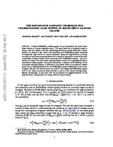
a constant exponential term as in (2), thus forming a family of parameterized ellipsoids[18] (see illustration for k=2 in Figure 1). The constant parameters z, µk and σk fully characterize the ellipsoid.

∑ k

( xk − µ k ) 2

= z2

σ k2

(2)

Applying a change of variable Xk = (xk -µk )/ σk , (2) now represents a hyper-sphere with respect to Xk in a space of dimension k (or k-sphere), and z is its radius. In the following, for the convenience of notations, we will always consider variables normalized to the standard N(0,1) distribution, unless otherwise specified. The choice of hyper-spherical coordinates to represent the samples is then the most natural one: the k Cartesian coordinates are represented by a radius z and (k-1) angles θ i [19]:

X 1 = z ⋅ cos(θ1 )

X 2 = z ⋅ sin (θ1 ) ⋅ cos(θ 2 )

X 3 = z ⋅ sin (θ1 ) ⋅ sin (θ 2 ) ⋅ cos(θ3 )

(3)



X k −1 = z ⋅ sin (θ1 )sin (θ k − 2 ) ⋅ cos(θ k −1 )

X k = z ⋅ sin (θ1 )sin (θ k − 2 ) ⋅ sin (θ k −1 )

Using such hyper-spherical coord inates (3) and normalized variables (or µk =0, σk =1), the PDF (1) now simp ly reads: z2

− 1 2 ⋅ f ( z ,θ i ) = e k/2 (2π )

(4)

Iso-density ellipse

2. Construction of the Sampling Method 2.1. The Multi variate Normal Distribution The lack o f in formation on the responses does not prevent calculating a probability of occurrence of events in a mu ltivariate problem. The idea of XES is to do so in order to over-sample rare events and thus enhance the CDF calculation for far quantiles as compared to a CMC sampling. In order to identify such rare events, we first have to establish the joint probability of a set of random variab les (xk ). With the assumptions that all input variables are normally distributed and independent, the mu ltivariate joint Probability Density Function (PDF) of a set xk of such variables (xk ~ N (µk ,σk 2 )) reads[18]:

= f ( xk )

1

( 2π )k /2 ⋅ ∏ σ k

⋅e

−

1 ( xk − µk ) ∑ σ2 2 k k

2

(1)

k

Iso-density curves for such a PDF are defined by assuming

Figure 1. Example of bivariate probability density function with an iso-density ellipse highlighted. X, Y ~ N(0,1). X/Y scales in standard sigma

As expected, since the hyper-spheres represent iso-density curves (radial symmetry of the density of probability), (4) shows no dependence to the (k-1) angles θi of the system. As a consequence, calculating the Cu mu lative Distributio n Function (CDF) fro m (4) using these coordinates can be

International Journal of Probability and Statistics 2012, 1(4): 133-144

135

done regardless of the angular position and with a single classical Monte-Carlo technique[21], we can then co mpute variable of integration: z. It also implies that a g iven k-sphere the emp irical probability F(ξ) fo r a response R(Xk ) to be is not only an iso-density surface but also an iso-probability lower than ξ fro m the following discrete sum (in other words: surface. Finally, since the variable z represents the distance the discrete CDF of R): fro m the center point o f the parameter space (z=0 means all = F (ξ ) P R ( X k ) < ξ variables are at their average value), lo w probability events (10) z2 of interest for XES corresponds to high z values – this aspect N 1− k /2 − i 2 i k − 1 is further commented in section 2.5, especially as regards = the ⋅ zi ⋅ e 2 ⋅ dz I R Xk < ξ ⋅ / 2 ⋅ Γ n z k ( ) ( ) case of circuit analysis. i i =1 In the proposed technique, we take advantage of these for a given series of rad iuses zi and a constant stepping dz, properties to calculate the CDF of responses of mu ltip le and with N being the total number of samp les: variables, using randomly chosen samples on concentric z max hyper-spheres and a modulation of the sampling versus the N= n z (11) parameter z to enhance rare events in selected ranges of z = z min probability of occurrence. F(ξ) can also be written: We will now describe how to achieve such a sampling N plan in practice and how to calcu late the CDF of arbitrary F (ξ ) P R ( X k = I R X ki < ξ ⋅W ( zi ) ξ = < ) responses. i =1 (12) zi2 1− k /2 2.2. Marginal PDF on k-S pheres − 2

(

)

(( ) )

∑

∑ ()

(

Let’s first establish the natural density of samples on a given k-sphere, by calcu lating the follo wing marginal PDF (p z) of events for a k-sphere of radius z:

1

= ⋅e ∫ f ( z,θi ) ⋅ dV k /2 π 2 ( ) θi

= pz

−

2

z 2

⋅ ∫ dV

(5)

θi

where d V is the volu me element (Jacobian) of the k-sphere. In the hyper-spherical coordinates, d V reads[19]: k −2 k −1 (6) sin i (θ k −i −1 ) ⋅ dθ k −i −1 dV= z ⋅ dz ⋅ i =0 Hence, we can rewrite the integral in (5):

∏

k −1 ∫ dV= z ⋅ dz ⋅ ∫

k −2

∏ sini (θk −i −1) ⋅ dθk −i −1

θi i = 0

θi

(7)

= z k −1 ⋅ dz ⋅ Sk with Sk being, by defin ition, the area of the unit k-sphere[20]: ∞ 2π k / 2 Sk = , Γ(t ) = ∫ t z −1 ⋅ e −t ⋅ dt 0 Γ(k / 2)

(8)

As a result, p z reads:

= pz

∫

θi

z2

21−k /2 k −1 − 2 f ( z ,θi ) ⋅ dV = ⋅ z ⋅ e ⋅ dz (9) Γ(k / 2)

then, calculating the corresponding CDF fro m (9) requires integrating p z with z vary ing fro m 0 to +∞. 2.3. Empirical CDF Calcul ati on Let’s now introduce a function n(z) yielding a number of samples n for a given k-sphere radius z. Since the natural density of samples for a given sphere z is defined by (9), the corrected marg inal PDF for a such a samp ling plan equals p z/n(z). Taking into account the above and similarly to the

W ( zi ) =

) ∑

n ( zi ) ⋅ Γ ( k / 2 )

( ( ) )

⋅ zik −1 ⋅ e

2

⋅ dz

Such a formu lation is similar to Importance Samp ling techniques[3], W(zi ) representing the statistical weight associated to samples. In practice, the integration variable z is taken on a constant grid (dz constant), which also makes the integration method somewhat similar to a quasi-Monte-Carlo approach[21], but with a grid representing here equi-probable occurrences. Theoretically, the sum of weights thus defined (12) should exactly equal one. In practice, however, discrete summation and numerical error lead to significant deviations fro m this ideal situation, which suggests performing a normalization of weights to their average, as often reported in the literature[3][22]:

= F (ξ ) P ( R ( X k = ) ξ p  N i =1

 2  − p , p ≤ 0.5  (19) 2 Wi  2 ⋅ 2  − (1 − p ) , p > 0.5 W 

( ( )

) ⋅ WW

( ( )

)

2

i

2

For CM C, the asymptotic value of ψ2 reads[26]:

ψ p2 = p ⋅ (1 − p )

(20)

Fro m (18), the standard deviation of the p-quantile estimator (ξp ) reads:

σ= ξp

ψp 1 ⋅ N f ξp

( )

(21)

interval estimate (22) in the case of XES, we experimentally compared it to a CI calcu lated by re-sampling through a bootstrap (BS) technique and using Studentized statistics [27][28]. As we will illustrate in the next section, a good agreement is observed between the CIs calculated by the two methods. Finally, we define two gains (Ga, Gs) to measure the performance of XES over CMC:

Ga = Gs =

ε p (CMC ) ε p ( XES )

N CMC (ε p ≤ 0.15)

(24)

N XES (ε p ≤ 0.15)

Ga being the gain in accuracy at a given sampling N, and Gs the gain in sampling at a given relat ive error εp (15% in this case). We can notice that the gain Ga is the ratio of relative errors, which is actually equivalent to a classical metric measuring the gain of an IS over CM C at a given p-quantile for a constant number of samp les N: Ga~σMC/σIS[4].

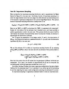
3. Empirical Study We imp lemented the above formu las and sampling scheme in a co mmercial nu merical co mputing platform in order to evaluate the accuracy and efficiency of the XES method, as we will now illustrate. The examp les shown hereafter are built around a series of simp le electrical test circuits made of resistors connected in series or in parallel and biased under a constant current Ic (Figure 7). The studied response is a voltage drop (Vd) across the circuit, and the random variab les are the resistances. These simp le circu its could represent, for example, a memory cell that would be repeated over a memo ry array and would experience statistical variat ions of its parameters (here: the resistance value). Since the equivalent resistance of such circuits is calculable, the response has a known analytical formu la (Figure 7). In the following examp les, this formu la is used to calculate the response Vd for each sample and hence reconstruct the CDF; in an actual imp lementation, a circu it solver would co mpute the responses. a/ Type 1

b/ Type 2

where ψp is calculated fro m (19) for XES or (20) for CM C. Then, to calculate a 95% CI, we used the classical approximation :

~ CI 95% = ξ p ± 1.96 ⋅ σ ξ p

(22)

In order to estimate the accuracy of estimated probabilities, we also calcu late the relative error εp on a g iven probability p[1]:

εp =

σp 1 ψp = ⋅ p N p

(23)

To further check the validity of the above confidence

Figure 7. Test circuit schematics with resistors in a/ series (s) (Type 1) or b/ series (s) and parallel (//) (Type 2). The equivalent resistance Req can be calculated in all cases using the classical formulas Req(Rx.s.Ry)=Rx+Ry Req(Rx//Ry)=Rx.Ry/(Rx+Ry). The studied response is the voltage drop Vd across the group of resistors under a constant current Ic (Ic=1mA in all the following examples): Vd=Req × Ic


Notes: probabilities in the CDF graphs below are expressed in sigma of the standard normal distribution, except otherwise specified. On such a scale, purely normal distributions show up as a straight line. The parameter dz in (12) is set to a constant value of 0.1 in all the examples below.

139

a/

3.1. Linear Response We will first illustrate XES in the case of a Type 1 circuit (Figure 7 a/) fo r which the response is linear with respect to the resistances, and for 3 resistors: R1, R2, R3, following normal (section 3.1.1.) o r non-normal (section 3.1.2.) distributions. 3.1.1. Normal Distributions

b/

The resistors are chosen as follows: R1:N(50,0.5²); R2: N(100,10²); R3:N(120,1.5²) – all values in oh m. The number of samples was set to 13,896 fo r the various plots below. Figure 8 shows the resulting XES CDF for Vd with the p low parameter set to 10-6 and for a targeted probability of 10-9 (assuming the studied population is of 1 b illion indiv iduals). Since in this case, the theoretical CDF can also be calculated fro m the co mposition of variance[18], we also plotted it in the same graph, in order to check that the two traces were superimposed. The 95% CI was also computed and is shown in Figure 9 together with the CDF for the lower (a/) and upper (b/) part of the CDF. The CI calcu lated with (22) and fro m a bootstrap re-samp ling gives consistent results. As expected, thanks to the XES strategy, the CI is narrow in the vicinity of the targeted probability, both at +6σ and at -6σ. The relative error on the estimated quantiles (δξ ) can also be calculated in this specific case, since the theoretical CDF and hence the true ξp are known :

Figure 9. Detail of a/ lower and b/ upper part of the XES CDF of Vd from Figure 8 as compared to the theoretical straight line; 95% CI calculated from (22) or from BS re-sampling (1000 runs)

~

δξ =

ξp −ξp ξp

(25)

With the above sampling plan, the measured δξ at ±6σ is well below 1% (typically around 0.1-0.2%).

Figure 10. Sampling plan for various p low, at a constant N=13,896

Refinement region

Targeted probability

Figure 8. CDF (sigma scale) of voltage drop (Vd) for 3 resistors / Type 1 circuit. The p tgt parameter is set to 10 -9 and p low to 10 -6 . XES CDF is superimposed to the theoretical straight line

Figure 11. Relative error εp vs. probability for various p low values at a constant N for CDF of Figure 8. The variations of p low modulate the refinement sampling range and the accuracy in this region

140


The effect of modulating the refinement region (Figure 10) through the plow parameter at a constant number of samples on the error εp is illustrated in Figure 11. The peak relative error observed in the 4-5σ range tends to decrease and to shift to lower σ for increasing p low , while the relat ive error degrades at the targeted probability of ±6σ. In this example, the criterion of εp < 15% at ±6σ is reached for plo w=10-6 . Another property of XES is evidenced in Figure 11: because of the symmetry of the sampling on k-spheres, both ends of the CDF are refined by over-sampling rare events corresponding to large z rad iuses, leading to an accurate estimation of p tgt (-6σ) and 1-p tgt (+6σ) together. This is a key feature to analyze responses showing a two-sided operating range (i.e. both low and high values leading to circuit failure). Figure 13. XES and CMC CDF of the response Vd of 3 resistances As already mentioned before, we exclude fro m this study the following 3-parameter Weibull distributions, Type 1 circuit particular cases of responses exhibit ing far quantiles at low z-values (specific non-monotonic functions), for wh ich the a/ above sampling refinement would not be effective on the lower (or upper) side of the CDF. 3.1.2. Non-No rmal Distributions Resistor 1

b/

Resistor 2

Figure 14. XES CDF of Vd and 95% Confidence Interval from (22) for a/ lower and b/ upper part of the CDF

Resistor 3

Figure 12. PDF of the resistances R1, R2 and R3 (Weibull distributions)

In this examp le, the circuit is identical to the previous (3 resistors in series) and resistances are simply changed to 3-parameter Weibull (W) distributions instead of normal, as follows: W R1 (scale=1, shape=1.5, location=50), W R2 (scale= 1, shape=30, location= 100), W R3 (scale=1, shape=4.5, location=120). The values were chosen to yield various PDF asymmetries, as illustrated in Figure 12. The XES parameters are: N=13,872 samp les, p tgt =10-9 , p low =10-4 . The resulting XES CDF is shown in Figure 13 and is superimposed to the CMC trace. The confidence interval in the lower and upper part of the CDF are shown in Figure 14, further illustrating the good accuracy obtained at extreme quantiles even for non normal d istributions.


3.2. Non Linear Response Considering now a Type 2 circu it and three normally distributed resistances, the resulting response Vd is non-linear, due to the resistors in parallel (Figure 7). In the following examp le, the resistances are chosen identical to the ones of section 3.1.1. The sampling plan is also similar, with p tgt =10-9 , p low =10-5 and N=13,880 samples. The CDF of the response are shown in Figure 15 together with the 95% CI calculated fro m (22) or with 1000 BS runs. Tight CIs are obtained in the targeted probability range and the two CIs are consistent. a/

b/

141

through a feedback of the response on the sampling while running). On the contrary, XES is built to deal with mu ltip le arbitrary responses with a single set of samp les, as we will now further illustrate on an examp le. Let’s consider 5 different responses of 3 normally distributed variables, built as follows: Vd1 is a linear response (Type 1 circuit) identical to section 3.1.1. Vd 2 is identical to section 3.2 (Type 2 circu it), Vd 3 and Vd4 are also fro m a Type 2 circuit but with a cyclic permutation of resistances as compared to Vd 2. Vd 5 is a purely fake response, built fro m the sum of square of resistances mu ltip lied by a constant (10-6 ), in order to illustrate the case of a response that is non linear and non-monotonic with respect to all its variables. As shown in Figure 17, despite the collection of responses yielding a large variety of CDF shapes, XES allows calculating all of them fro m a single set of samples. Moreover, in the sampling refinement region (p low =10-4 ; p tgt =10-9 ), the relative error εp is lo w and is similar for the various responses, as illustrated in Figure 18, proving the effectiveness and robustness of the method to arbitrary response shapes.

Figure 15. XES CDF of Vd and 95% confidence interval from (22) and from BS using 1000 runs (insets: detail of the a/ upper and b/ lower part of the CDF). Type 2 circuit with 3 resistors identical to section 3.1.1

Refinement region

Figure 17. CDF of various responses, single sampling plan, p low, =10 -4, N=13,989. The responses have been normalized (shifted to their median) in order to represent the various responses on the same x-scale

Figure 16. Relative error εp vs. cumulative probability (sigma scale)

Finally, the relat ive error (εp ) curve shown in Figure 16 clearly demonstrates the effect of the sampling refinement on the accuracy and illustrates that εp ~15% at p tgt =10-9 is reached for these sampling conditions, hence proving the effectiveness of XES also for non linear responses. 3.3. Mul ti ple Res ponses, Single Sampling Plan In cases where the response has a known analytical formula as in the above examp les, IS approaches such as exponential twisting[29] or mixture IS[8], for example, would certain ly be more efficient, but restricted to one response at a time, as the sampling is adjusted to the response shape (either by knowing the response beforehand, or

Figure 18. Relative error εp for the various responses Vd1 to Vd5, single sampling plan, p low, =10 -4 , p tgt=10 -9 , N=13,989

3.4. Larger Number of Vari ables (k)

142


As mentioned in section 2.5, the area of a k-sphere is growing rapidly with k and z, hence the number of samples required by XES is expected to gro w accordingly for far quantiles. We have empirically studied the evolution of the minimal sampling to reach a g iven relative error (εp